How to Teach Probability
This guide is for teachers who use CommeUnJeu with a class, from the first bags of counters of PYP 0 to the random variables of the Diploma Programme. It follows one idea through every year: an event is a set of outcomes, and its probability is a number attached to it. Before a pupil computes a probability, the pupil circles the outcomes that make the event happen; only then does the pupil count. When a chapter studies the frequencies of repeated trials, they come last, as what they are: a statistic that estimates a probability or puts a model to the test. In each chapter you will find:
- in most sections, a short video first, in English and in French (this guide shows them too, at the head of the passages they belong to);
- the lesson: definitions, methods and worked examples, to project on the board;
- under each section, the skills to practise: groups of exercises corrected at once, each answer followed by a worked correction;
- at the end, a quiz and, from PYP 1 on, a Going further section with harder problems;
- some exercises are written on paper: the pupil sends a photo of the page to have it corrected.
One Drawing, Two Objects
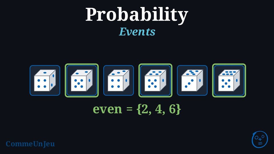
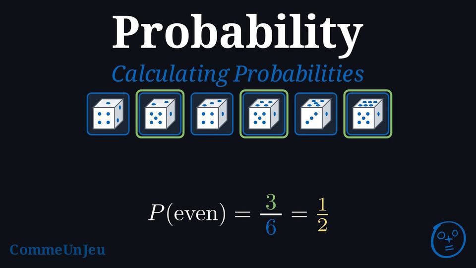
One roll of a fair six-sided die. “Rolling an even number” names an event: the faces \(2\), \(4\) and \(6\), the outcomes that make it happen. Its probability is a number between \(0\) and \(1\), here \(\dfrac{1}{2}\). The figure keeps the two objects in two frames, joined by one arrow. 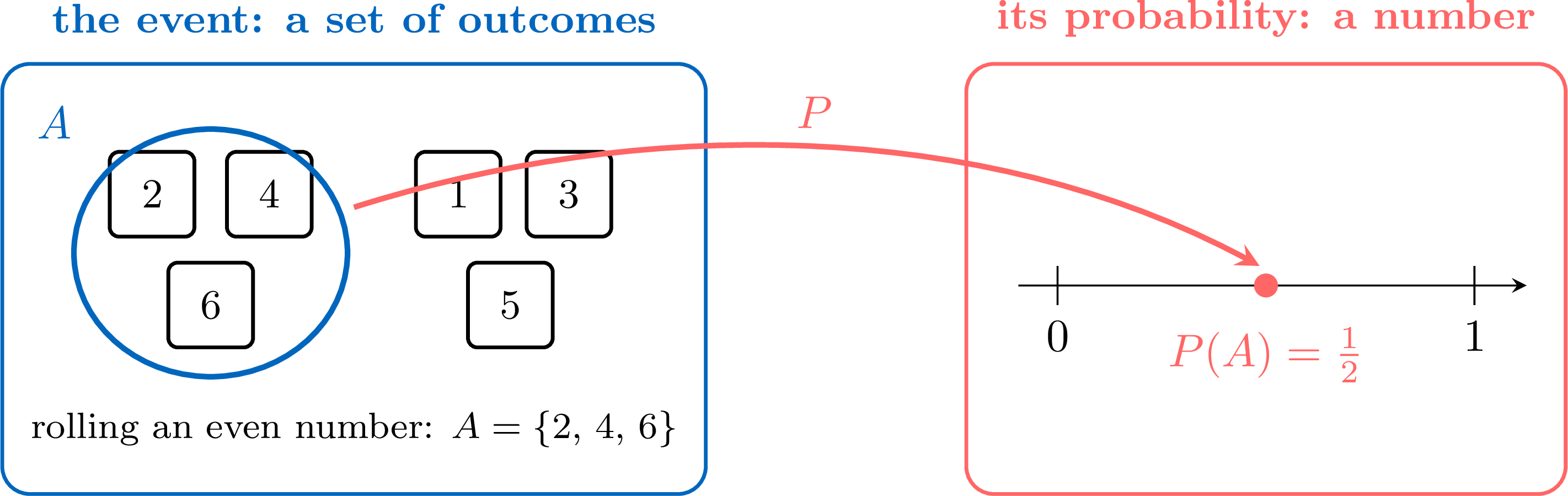
The event is the hoop and what is in it; the probability is a point on a line. Two sentences pupils write show whether they keep the two apart:
- “the event is \(\dfrac{1}{2}\)”, or \(A = \dfrac{1}{2}\): an event is never a number;
- \(P(A) = \{2, 4, 6\}\): a probability is never a set.
Three Gestures Throughout the Path
Three gestures guide the whole path, in this order. They are introduced according to the year and the content of the chapter: the details change, the order does not. 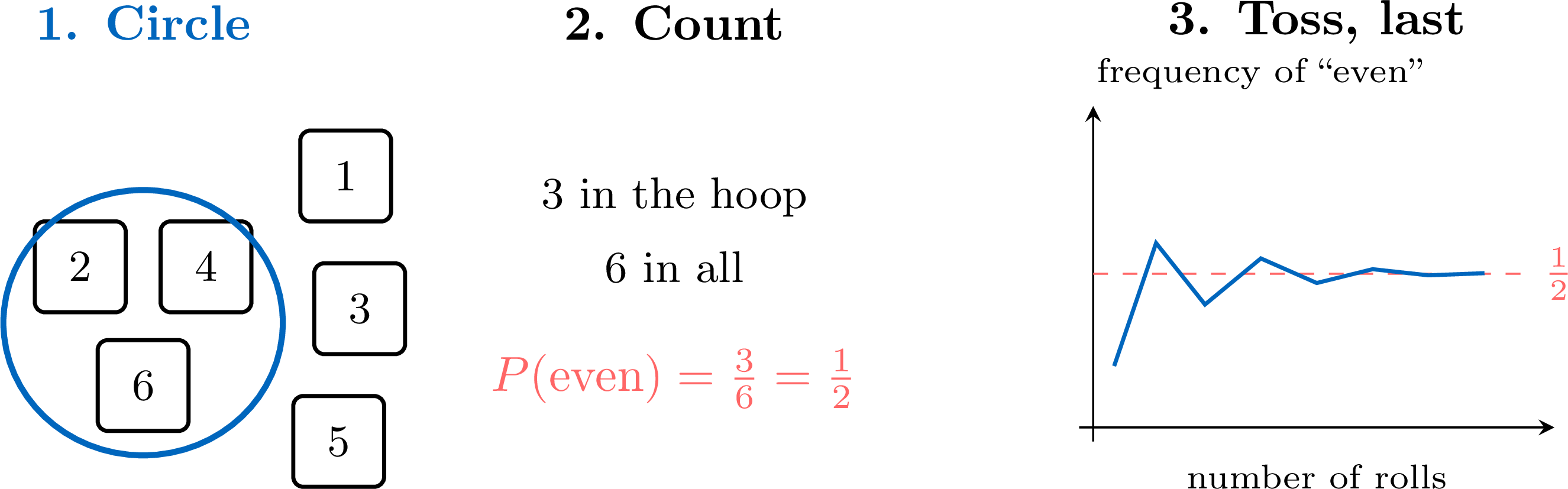
- Circle. Put in a hoop the outcomes that make the event happen. This is the event, built by hand.
- Count. When the outcomes are equally likely, count the outcomes in the hoop and all the outcomes, and divide.
- Toss, last. Repeat the experiment to estimate a probability, or to compare the frequency with a probability already calculated. This comes at the end of the chapter: the frequency estimates a probability, which may have been calculated before or may still be unknown.
Circle: Build the Event
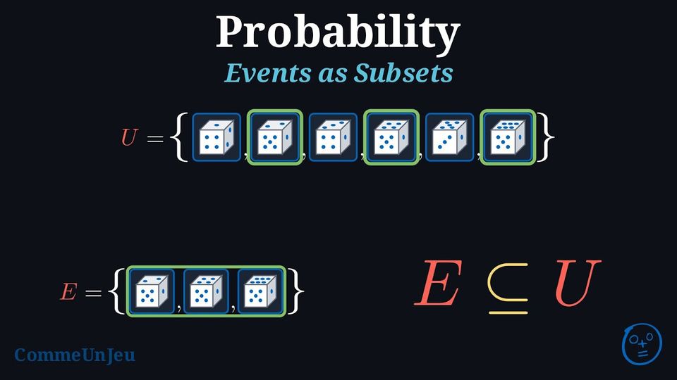
The hoop is the same object at every age; only its name changes. In PYP 0 it holds the red counters of a bag; in PYP 5 the cells of a table; from MYP 2 on it is written with braces, \(E = \{2, 4, 6\}\), a subset of the sample space \(U\); from MYP 3 on it is also a region of a Venn diagram. 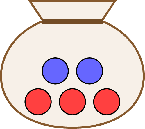
Ask for the hoop before any number, and ask for it on paper: “which outcomes?” is answered by a list, a drawing or a set, never by a fraction. The worked answers of the lessons always do it: “the outcomes for the event `rolling an even number' are \(2\), \(4\) and \(6\)”. From MYP 3, the method of every calculation has two steps: determine the event (list its outcomes, write it as a set), then compute its probability. In PYP 4, PYP 5 and MYP 1, several calculation exercises corrected online first ask for the number of favourable outcomes and the total number of outcomes.
Count: the Right Outcomes, Then Favourable over Total
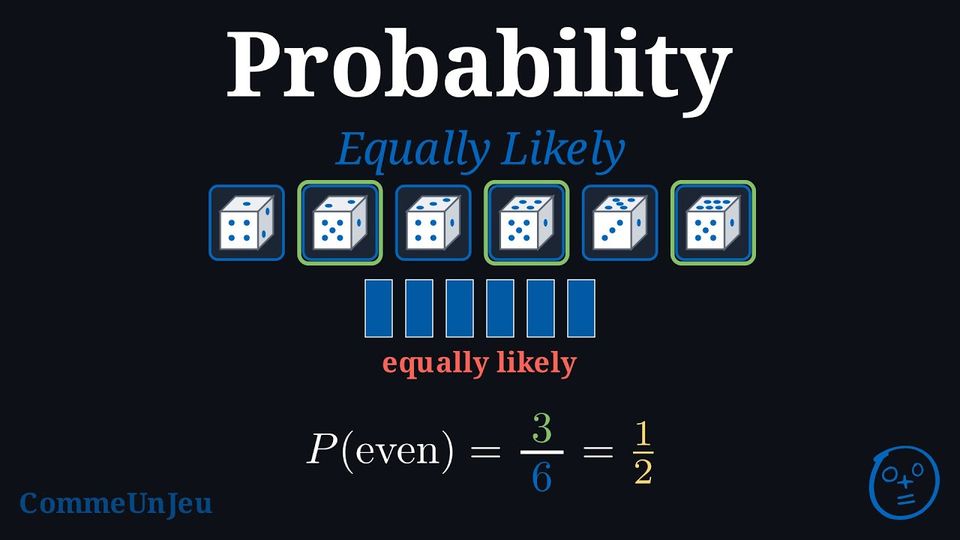
“Favourable over total” is true only when the outcomes counted are equally likely. The two spinners of PYP 3 show it. On A, \(6\) equal parts, numbered from \(1\) to \(6\); “red” is the set of parts \(1\) and \(2\): \(P(\text{red}) = \dfrac{2}{6}\). On B, three colours, but red covers half the circle: \(P(\text{red}) = \dfrac{1}{2}\), not \(\dfrac{1}{3}\). 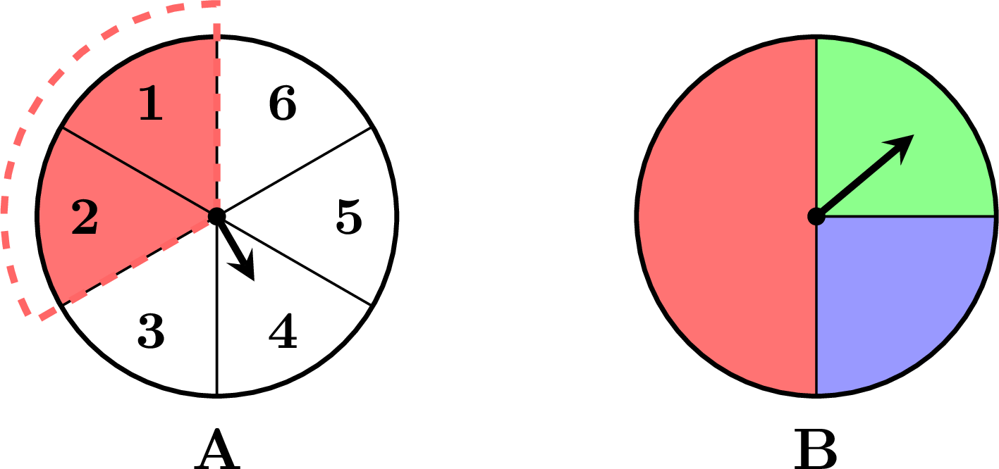
The same holds for a bag. With \(2\) red, \(1\) blue and \(1\) yellow counter, the three colours can be taken as outcomes, but they are not equally likely; to calculate by counting, take the four counters, which are. 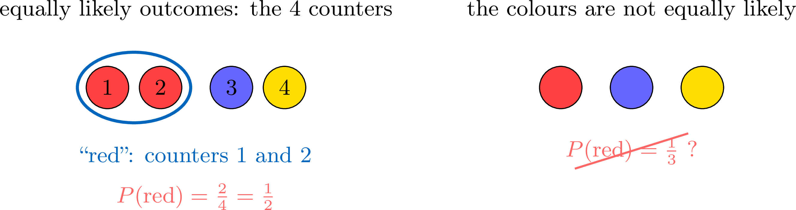
Once the outcomes are right, the rules of probability are facts about the hoops, read on the drawing before they are written as formulas. An event and its complement share out the sample space: their probabilities add up to \(1\). In \(A\) and in \(B\) taken separately, the outcomes of \(A \cap B\) are counted twice: hence the addition relation. 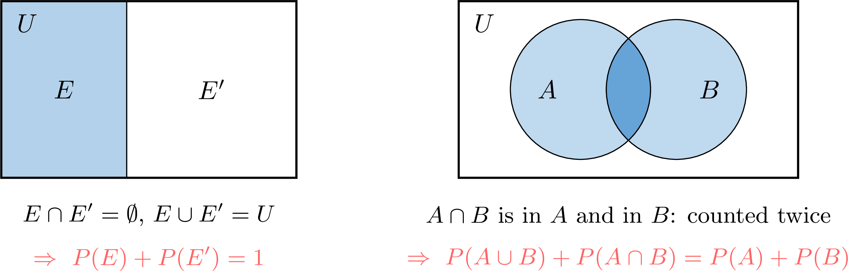
Toss, Last: the Frequency at the End of the Chapter
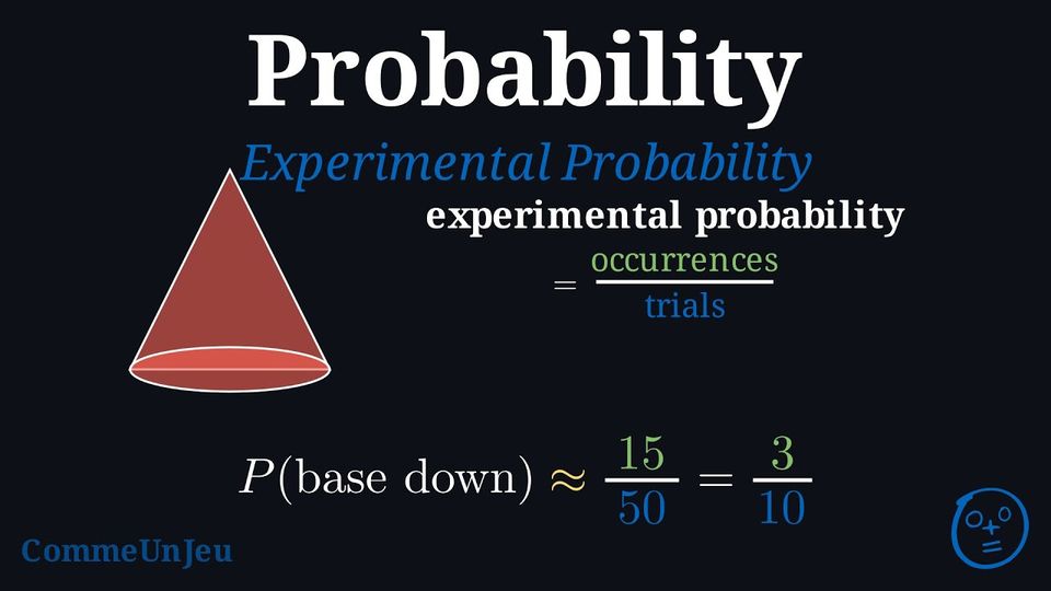
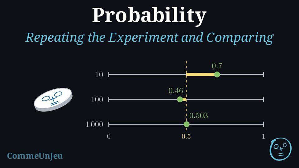
The frequency of an event in a series of trials is a statistic: the number of times the event happened, divided by the number of trials. It is not a second definition of the probability; it comes after the event and its probability, at the end of the chapter, and it serves two purposes. 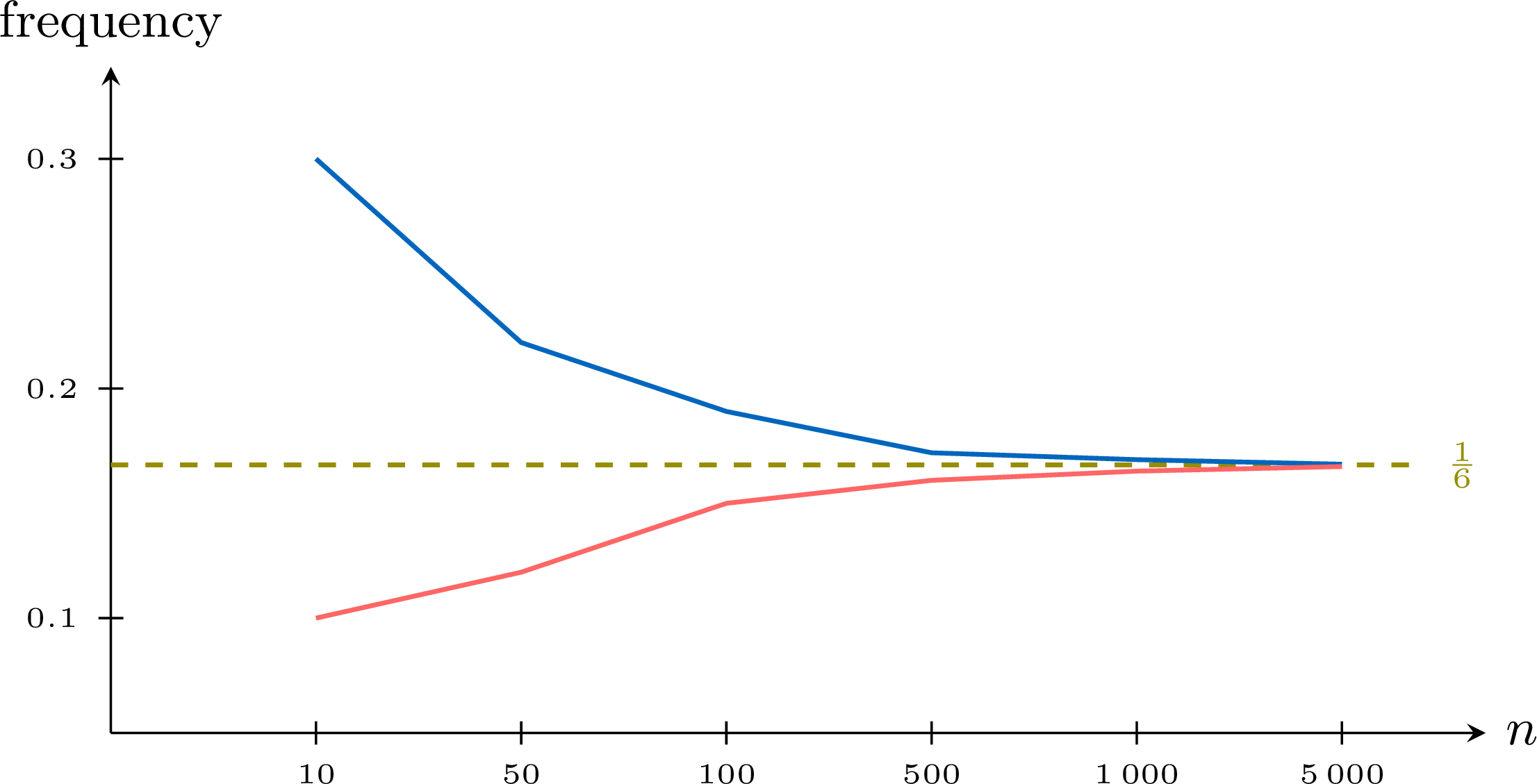
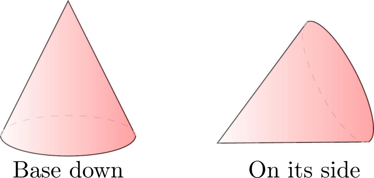
- It estimates a probability that no symmetry gives. A cone lands on its base or on its side, and the two are not equally likely. Isaac drops it \(50\) times: \(15\) times on its base, so \(P(\text{base down}) \approx \dfrac{15}{50}\). The probability exists before the trials; the frequency estimates it.
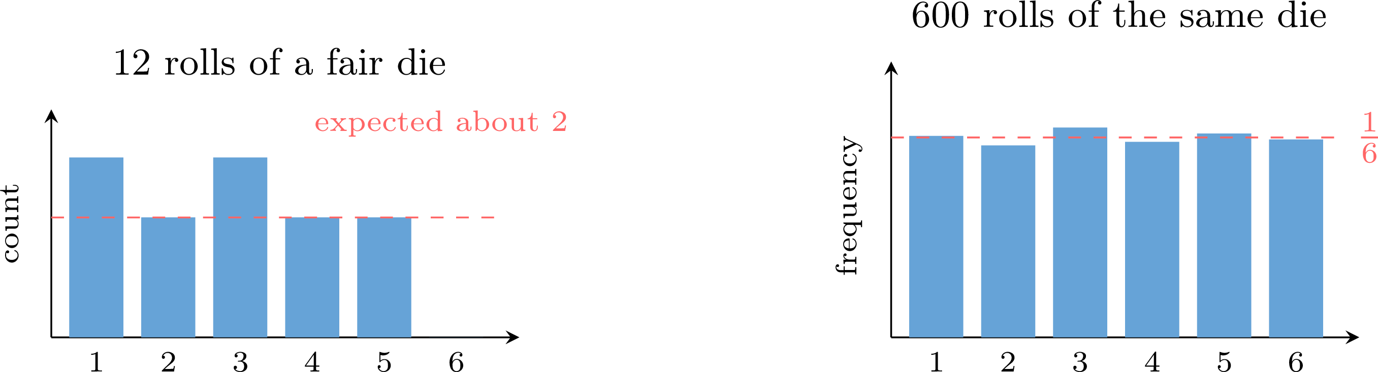
- It puts a model to the test. Léa rolls a fair die \(12\) times and gets no six. Neither “the die is loaded” nor “I should have had exactly two sixes” is right: twelve rolls are few, and a gap on its own proves nothing. Over hundreds of independent rolls, the frequency is usually close to \(\dfrac{1}{6}\).
The Path, Year by Year
Each chapter takes up what the year before taught, then goes one step further. Three strands run side by side: the events, from PYP 0; the numbers, from PYP 3; the frequencies, from PYP 3, always at the end of the chapter. 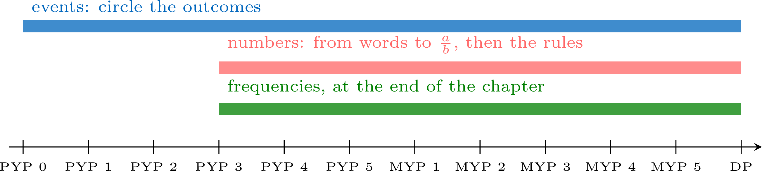
The DP rows link the Analysis and Approaches SL course; the three other DP courses have the same chapters, built from the same blocks.
| Year | Chapter | What is new |
| PYP 0 | Sorting, Picture Graphs and Chance | picking without looking: all, some, none |
| PYP 1 | Chance | what can come out; a bag built for an event |
| PYP 2 | Chance | not, or, and with two hoops; five words |
| PYP 3 | Chance | outcomes, events; a number from \(0\) to \(1\) |
| PYP 4 | Probability | favourable over total; fair games |
| PYP 5 | Probability | two steps: table, tree; no memory |
| MYP 1 | Probability | three forms; the probabilities add up to \(1\) |
| MYP 2 | Probability | the sample space \(U\); the complement |
| MYP 3 | Probability | events as sets; Venn; tables of pairs |
| MYP 4 | Probability | or, and; trees; expected gain; simulation |
| MYP 5 | Probability | the algebra of events; the axioms |
| MYP 5 | Conditional Probability | probability given an event |
| DP 1 | Probability | the world of events before the numbers |
| DP 1 | Conditional Probability | two-way tables; total probability |
| DP 2 | Discrete Random Variables | a function on \(U\); the binomial |
Year by Year, with the Figures of the Lessons
Before Numbers: the Bag and the Hoop (PYP 0 to PYP 2)
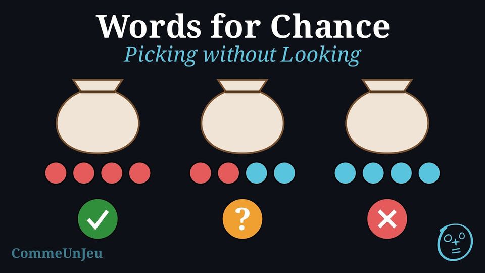
Concrete. A cloth bag and some counters that the children can see and touch. Before each draw, empty the bag on the table, ask “will the counter be red?”, then put the counters back and draw without looking. Pictorial. The PYP 0 method decides by looking at all the counters: if all are red, picking a red counter is certain; if some are red and some are not, it is maybe; if none is red, it is impossible. The judgement is made on a set, before any number. 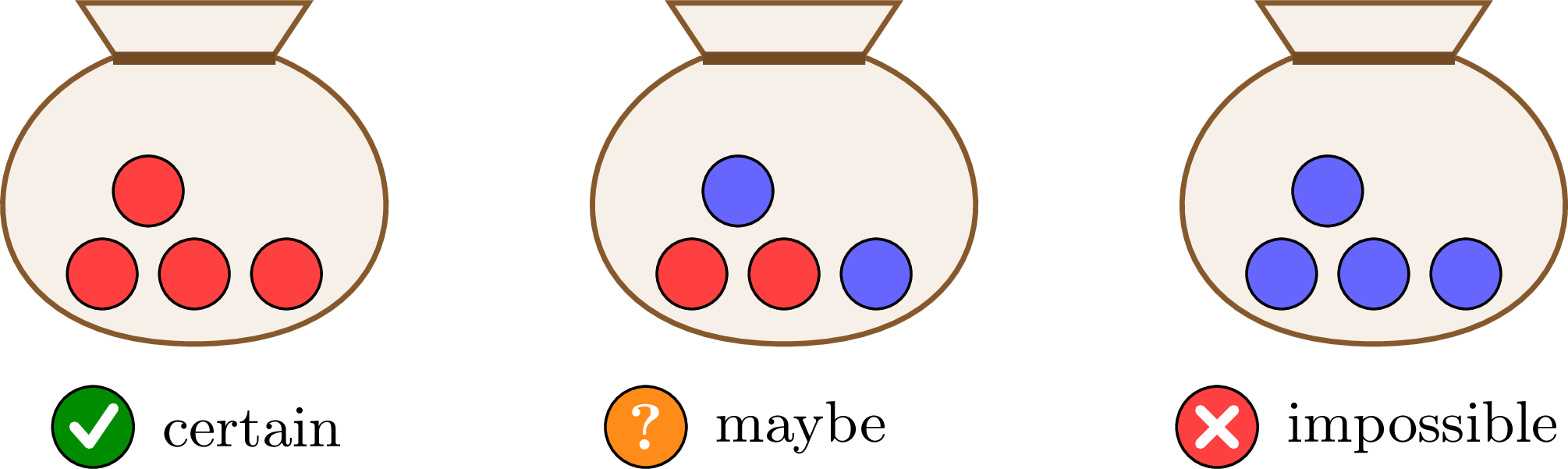
Then the hoop: “which counters make `the counter is red' happen? Put them in the hoop.” PYP 1 does the same with a die and a spinner: first everything that can come out, then the hoop, then the comparison of the hoop with everything. The hoop holds \(2\) of the \(6\) faces: getting more than \(4\) dots is possible. 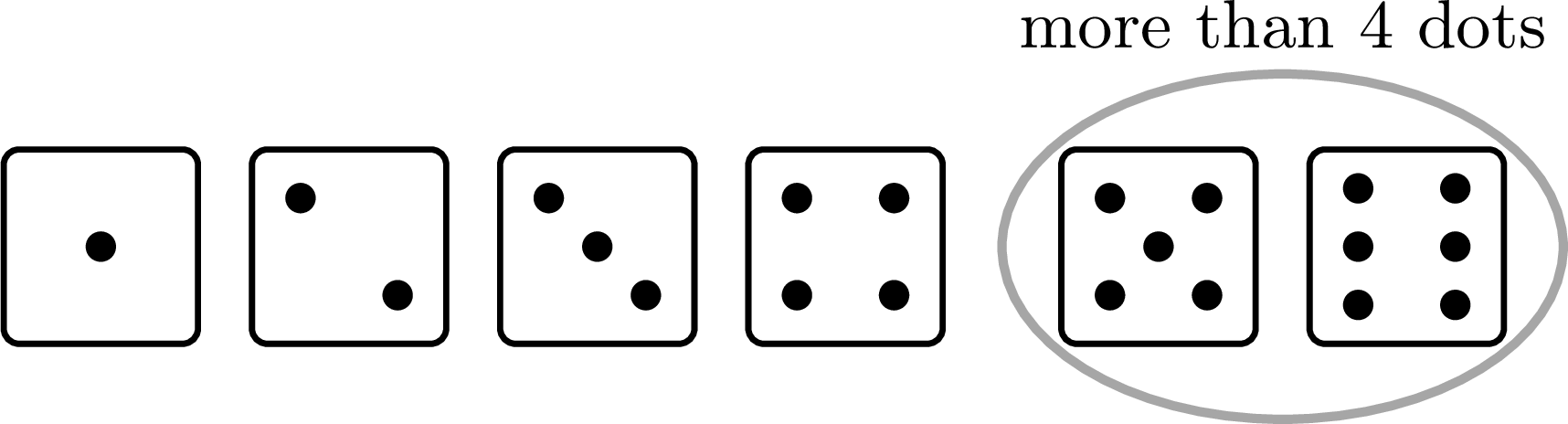
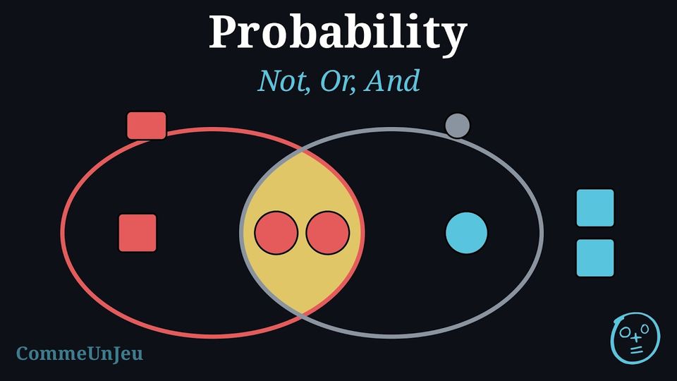
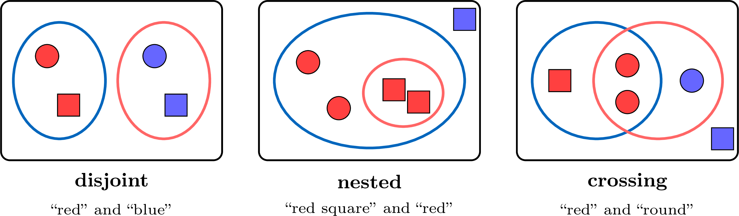
In Building the Bag, the pupil colours the marbles so that picking a red one is certain, then impossible, then possible but not certain: the event is built before it is judged. PYP 2 adds not, or, and. Two hoops, “red” and “round”: “not red” is outside the first hoop; “red and round” is where they cross; “red or round” is in at least one of them. “Red or not red” holds every counter: certain. “Red and not red” holds none: impossible. 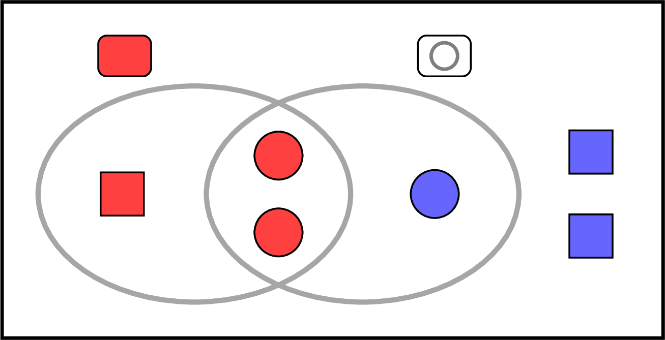
The same with a die: \(A\), “more than \(4\)”, and \(B\), “even”. 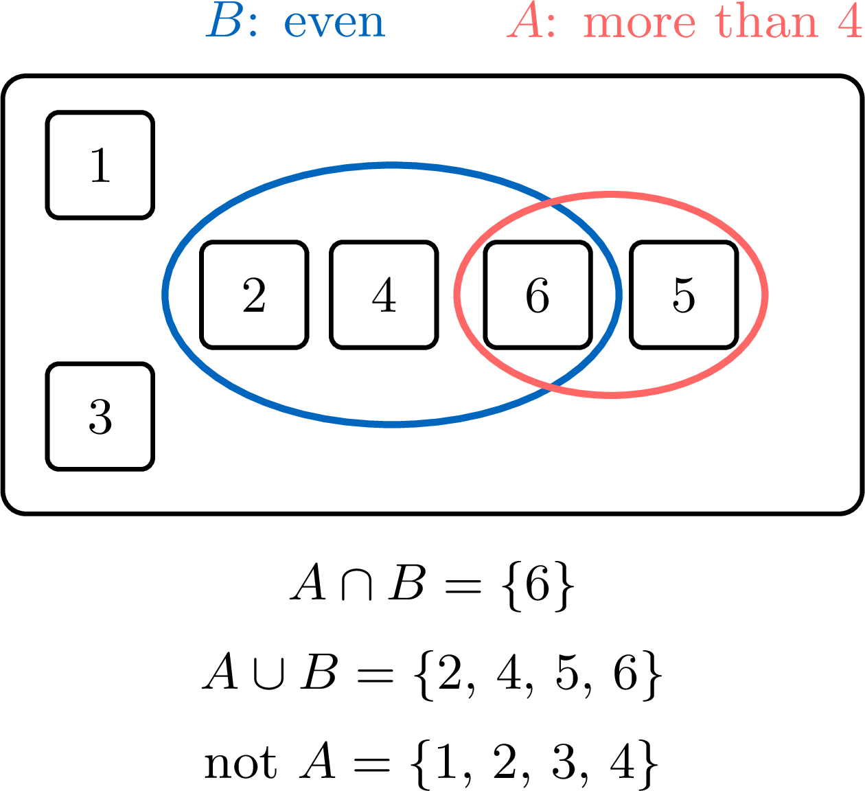
Last, the counts in the bag, for the line from impossible to certain: with only red and blue counters, each with the same chance, as many red as blue is an even chance. The lesson warns that both conditions matter: with \(1\) red, \(1\) blue and \(2\) yellow counters, red is less likely, not an even chance. 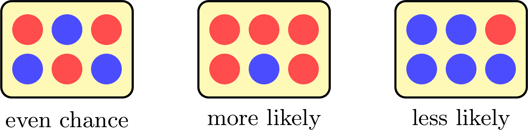
Abstract. No symbol yet. The words are the abstraction: certain, possible, impossible, said of a hoop compared with the whole bag. Where to find it. PYP 0, Sorting, Picture Graphs and Chance: Picking without Looking, with the exercises Filling the Hoop and Picking a Counter. PYP 1, Chance: What Can Come Out? (Showing Everything That Can Come Out, Filling the Hoop), then Certain, Possible or Impossible? (Picking at Random, Building the Bag). PYP 2, Chance: Not, Or, And (Finding the Counters That Are Not…, Using Two Hoops), then From Impossible to Certain.
Outcomes, Events, then Words and Numbers (PYP 3 and PYP 4)
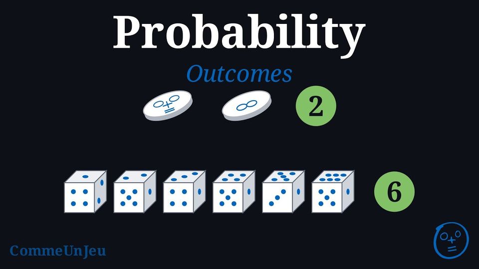
Concrete. A coin, a die. Ask for all the possible outcomes before anything else: heads and tails; the six faces. 
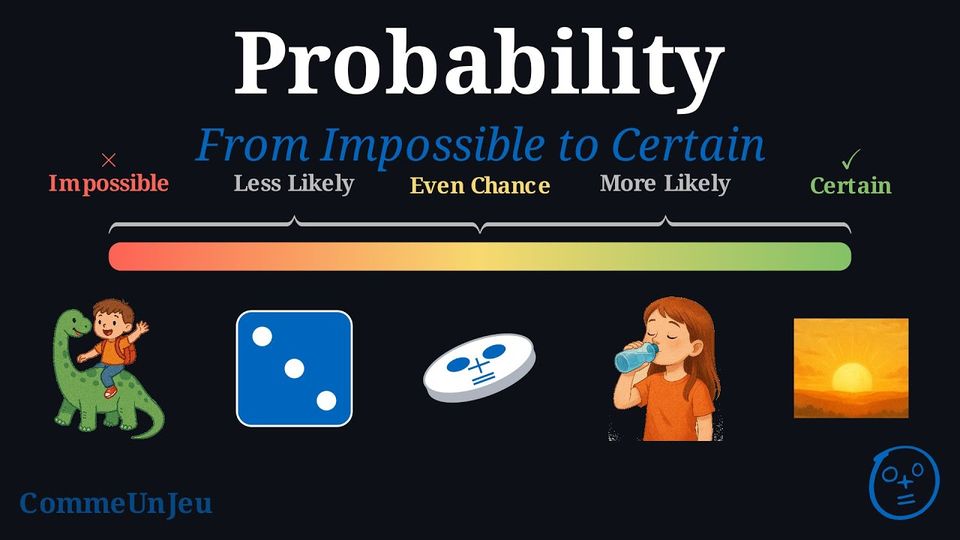
Pictorial. An event is “a set of outcomes”: rolling an even number is the faces \(2\), \(4\), \(6\). Then the line of five words, from impossible to certain. Its pictures come from everyday life, and the lesson says so: riding a dinosaur or the sunrise are everyday happenings, not events of an experiment; in an experiment, an event is impossible when no outcome makes it happen and certain when every outcome does. 
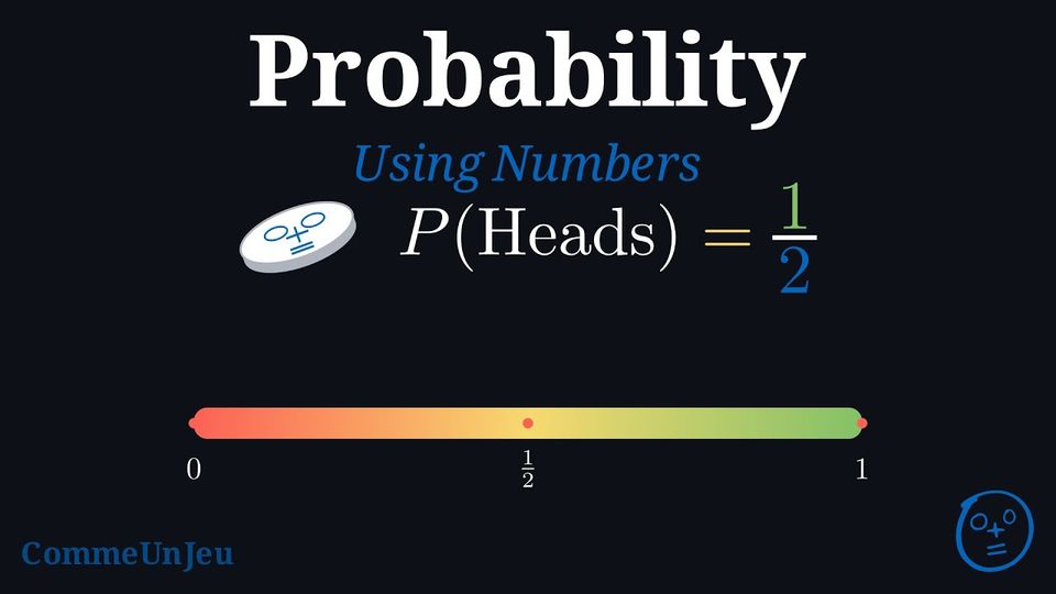
The number comes next: a probability is a number from \(0\) (impossible) to \(1\) (certain); with a fair coin, heads has a probability of \(\dfrac{1}{2}\). 
Abstract. When the outcomes are equally likely, \(P(\text{event}) = \dfrac{\text{number of favourable outcomes}}{\text{total number of possible outcomes}}\). Two events of the same experiment are compared by their favourable outcomes, since the total is the same: on this balanced spinner with \(8\) equal sectors, red has \(4\) sectors and blue \(3\). 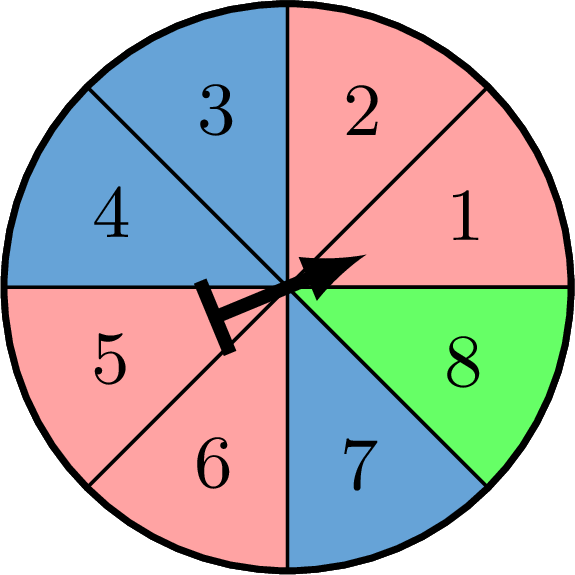
Where to find it. PYP 3, Chance: Outcomes, Events, From Impossible to Certain, Probability, a Number from 0 to 1 (with the exercise One Chance in n). PYP 4, Probability: Outcomes and Events, then Calculating and Comparing Probabilities, which opens on the probability as a number, with the exercises Calculating Probabilities and Calculating Probabilities on a Spinner. In them, the pupil first counts the favourable outcomes and all the possible outcomes.
Fair Games: Count the Winning Outcomes (PYP 4)
Concrete. Sam and Mia roll a fair die. Sam wins the round on \(1\) or \(2\), Mia on \(3\), \(4\), \(5\) or \(6\). Mia says the game is fair, since they roll the same number of times. Ask the pupils to check her claim by listing each player's winning faces. Pictorial. One hoop per player, on the same six faces. 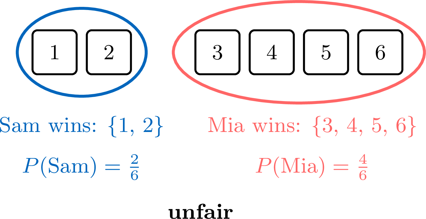
The spinner of the lesson asks the same question: Léa wins on red, Tom on blue or green. 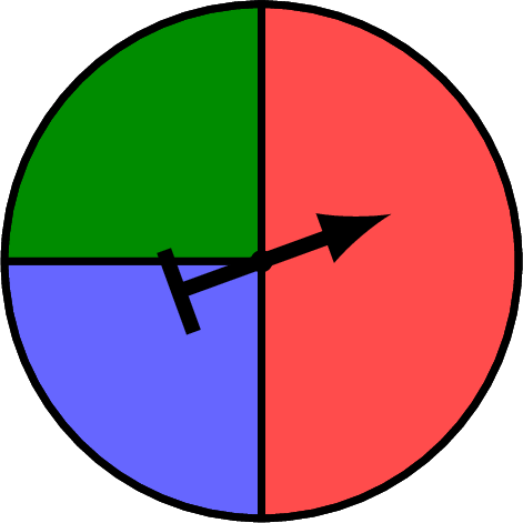
Abstract. A game is fair when every player has the same chance of winning. To decide: make the outcomes equally likely (a part twice as big counts as two equal parts), count the winning outcomes of each player, compare. To make the game fair, change the rules until the counts are equal. The winners of a few rounds do not decide it; the counts do. Where to find it. PYP 4, Fair and Unfair Games, with the exercises Deciding Whether a Game Is Fair and, written on paper, Making a Game Fair.
Two Steps, and the Die Has No Memory (PYP 5)
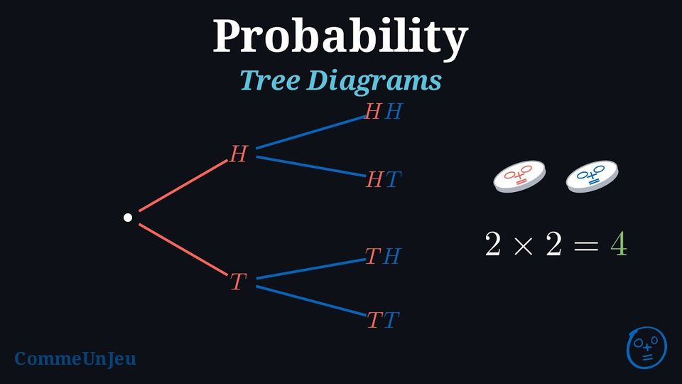
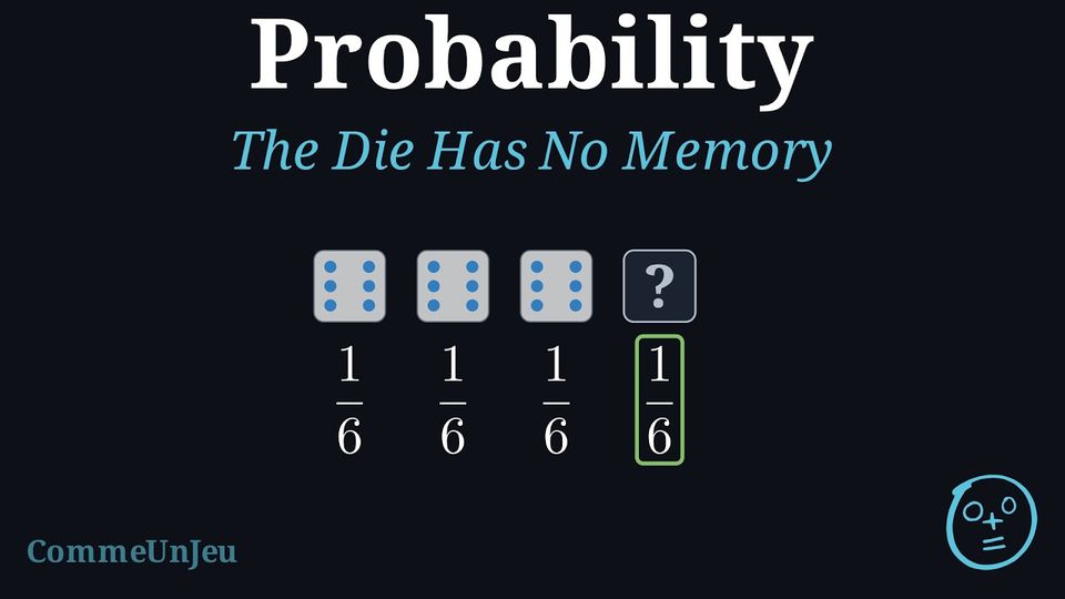
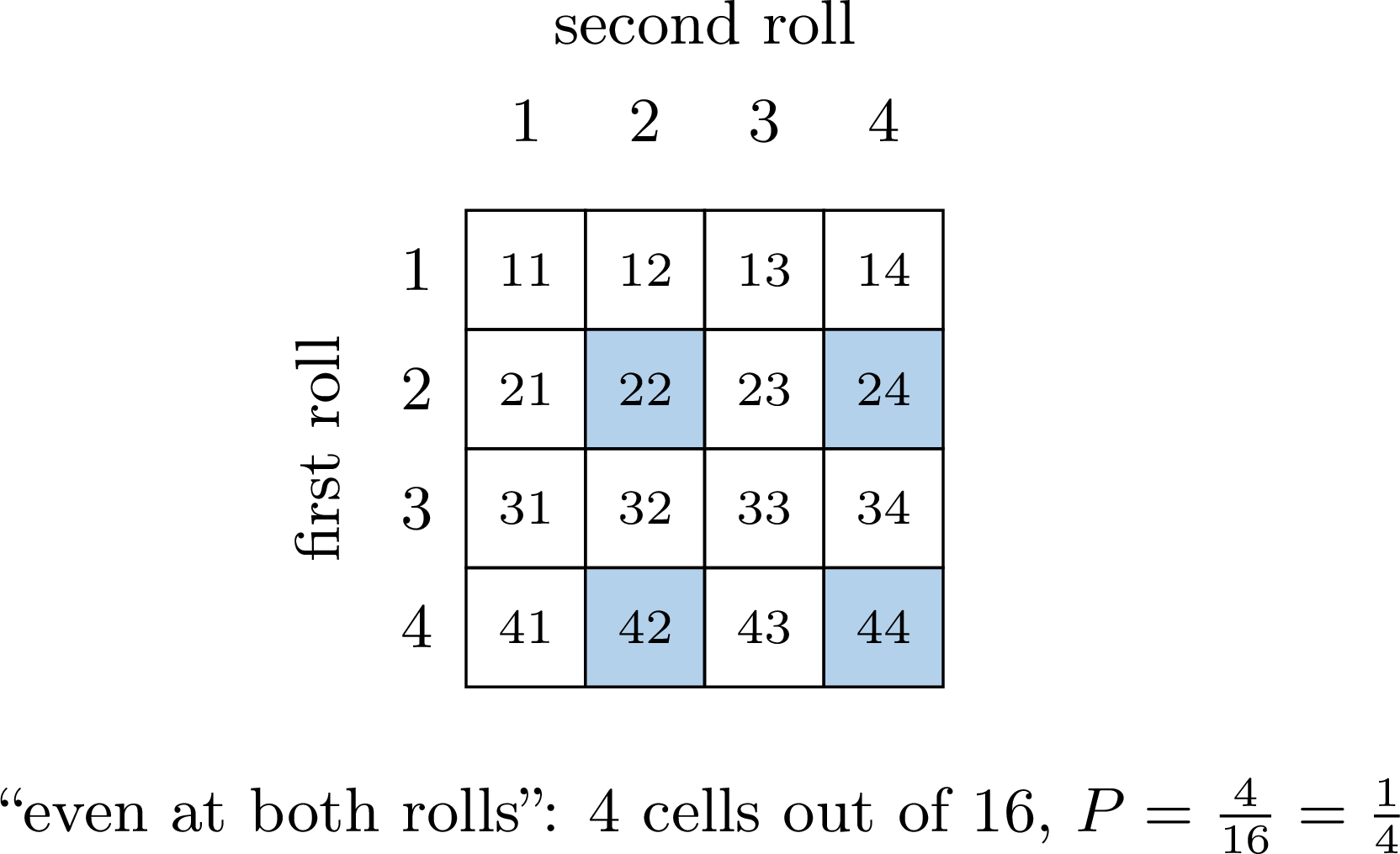
Concrete. Léa rolls a four-sided die, then rolls it again, and writes the two results side by side: \(11\), \(12\), \(13\)… She soon loses track. Let the pupils try it before showing any tool. Pictorial. An outcome of a two-step experiment is the pair made of a result of the first step followed by a result of the second. The table gives one row per first result and one column per second result: each cell is one outcome, and the number of outcomes is a product, \(4 \times 4 = 16\). The tree shows the order of the steps, and it keeps working for three steps or more. 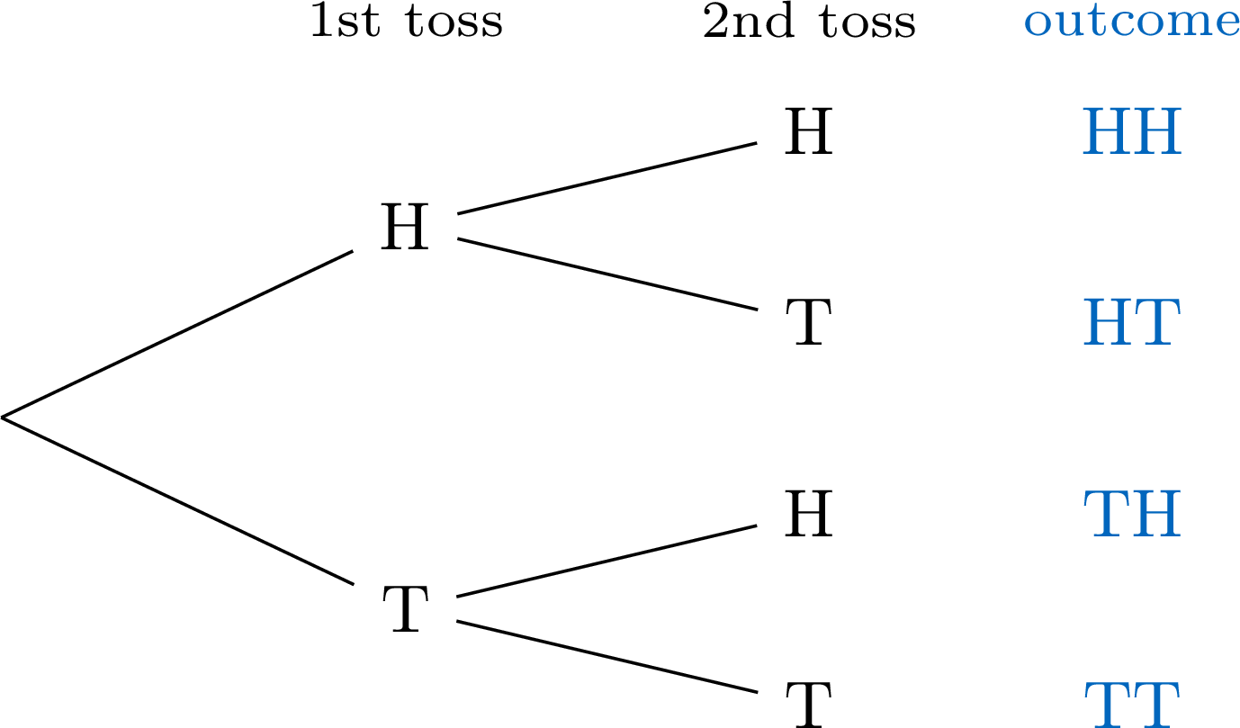
The product rule for counting holds because the second step has the same outcomes whatever the first gave: the same die is rolled again, the ball is put back in the bag. Abstract. Nothing new for the calculation: the cells of the table, or the ends of the tree, are the outcomes. Check that they are equally likely (each step is fair and the second is carried out under the same conditions as the first: we assume it), count those that realise the event, divide. “An even number at both rolls” is realised by \(4\) cells out of \(16\): \(P = \dfrac{4}{16} = \dfrac{1}{4}\). At the end of the chapter, a remark. Lina has rolled three sixes: 
“the next one will certainly not be a six”, she says; Sami answers that the die is lucky today. Neither: knowing the previous results does not change the chances of the next roll. PYP 5 and CM2 say it in a remark of their last section, not as a definition: independence is built later. Drawing without replacement gives an example of the opposite: the bag changes after each draw. Where to find it. PYP 5, Probability: Outcomes, Events and Two-Step Experiments (exercises Completing the Table of Outcomes, Reading the Tree of Outcomes), Calculating a Probability in Two Steps, then, last, Experimental Probability, which opens on the die that has no memory (Deciding Whether the Die Has a Memory, Calculating the Chances at the Next Trial).
One Number, Three Forms; Outcomes That Are Not Equally Likely (MYP 1)
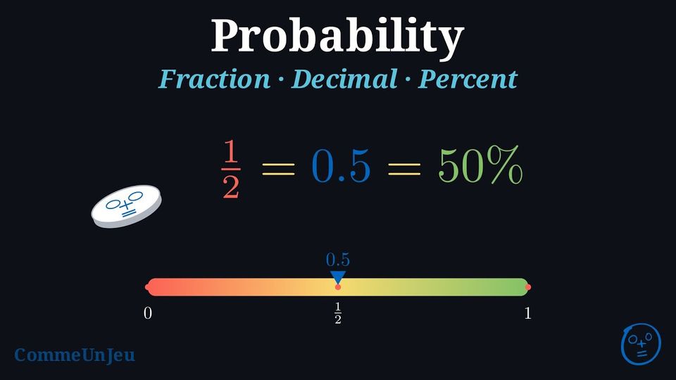
MYP 1 opens with Outcomes and Events, then describes probability in words and as a number, then calculates. Two things are new. Three forms of one number. A probability is written as a fraction, a decimal or a percentage; the three are the same number. The fraction is the exact form: \(\dfrac{1}{3}\) is not \(0.33\). 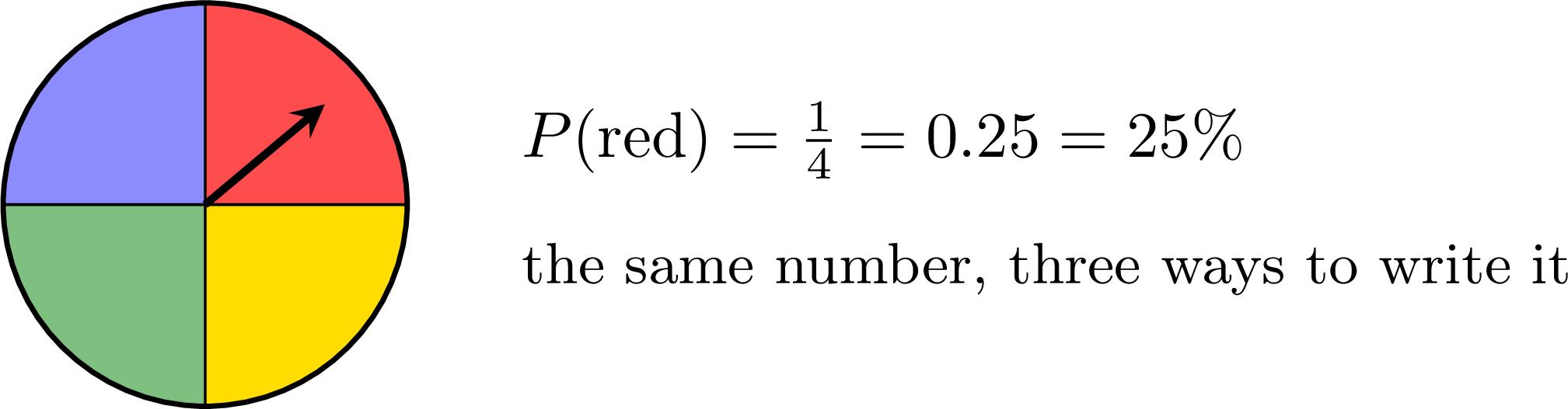
Outcomes that are not equally likely. On this wheel, red covers half, blue a quarter, green and yellow an eighth each. Lina says that each colour has a probability of \(\dfrac{1}{4}\), since there are four colours. The list of outcomes is the same as on a fair four-colour wheel; what has changed is the weight of each outcome. 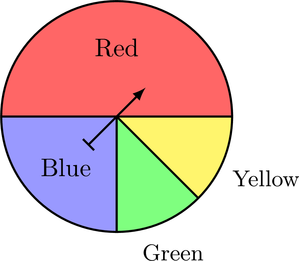
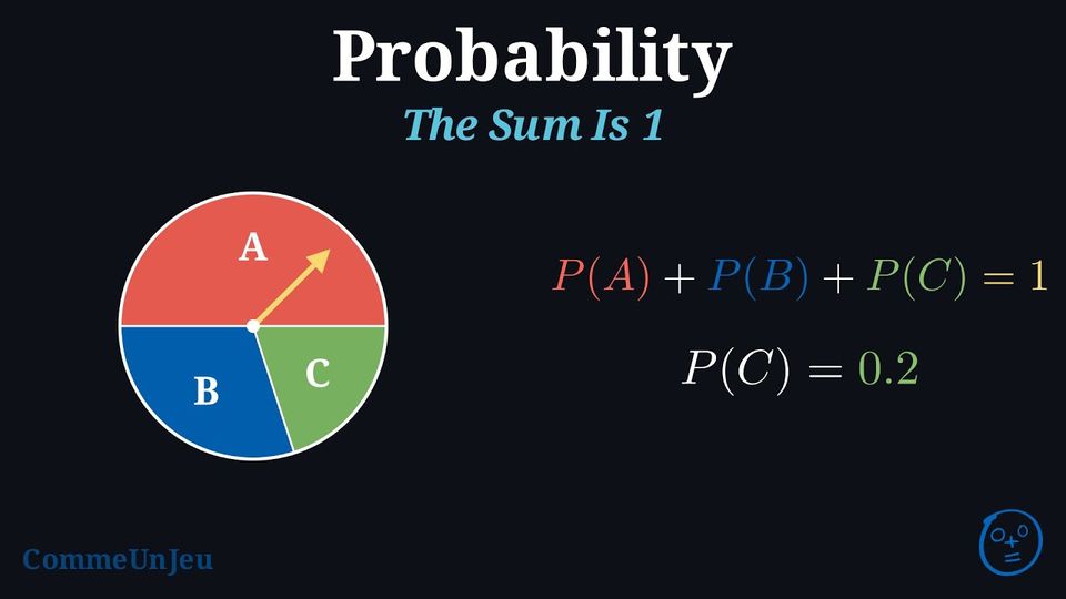
Abstract. The probabilities of all the outcomes add up to \(1\), and the probability of an event is the sum of the probabilities of its outcomes. For a spinner with exactly three outcomes \(A\), \(B\) and \(C\), the missing probability follows: \(P(C) = 1 - P(A) - P(B)\). Where to find it. MYP 1, Probability: Outcomes and Events, Describing Probability, Calculating Probabilities, whose subsections Equally Likely Outcomes, Three Ways to Write a Probability and The Probabilities Add Up to 1 each have their exercises.
The Sample Space, Singletons and the Complement (MYP 2)
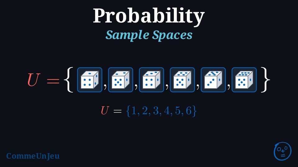
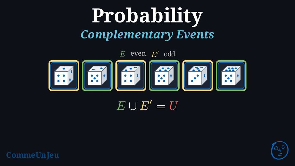
Concrete. One die. Ask the pupils to write all the outcomes between braces: the sample space \(U = \{1, 2, 3, 4, 5, 6\}\). Then “rolling an even number” as a set: \(E = \{2, 4, 6\}\), a subset of \(U\). Pictorial. An outcome and the event that contains only it are two objects: the face \(3\) and the singleton \(\{3\}\), “rolling a 3”. 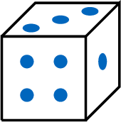
The complementary event \(E'\) is made of the outcomes of \(U\) that are not in \(E\). Every outcome lies in exactly one of \(E\) and \(E'\): the two share out the sample space. 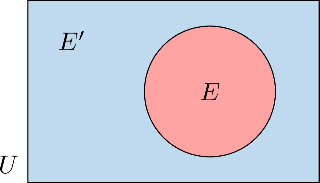
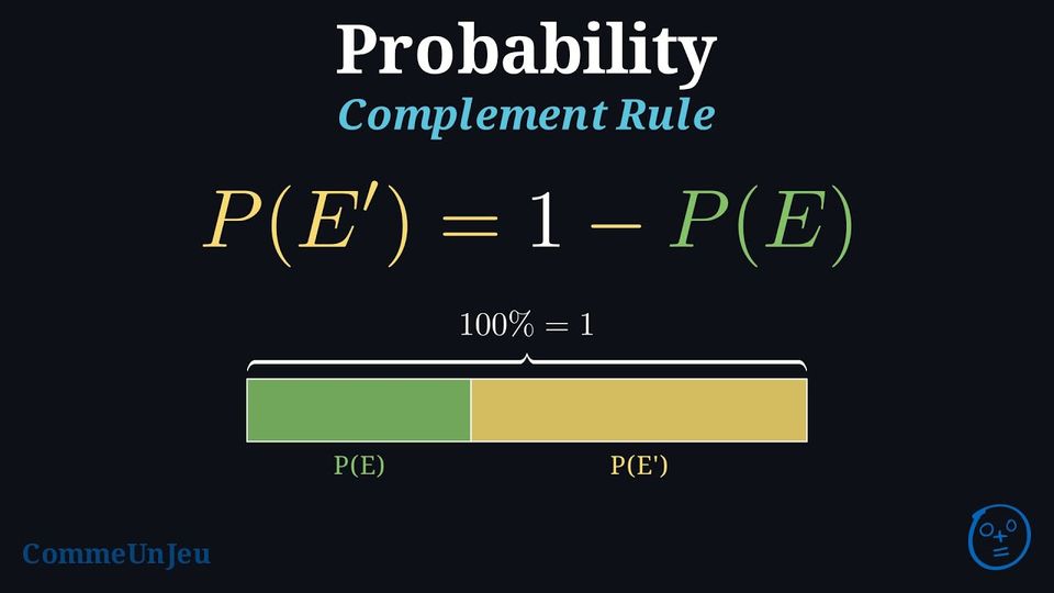
Abstract. The complement rule is proved from the drawing, not admitted: adding \(P(E)\) and \(P(E')\) counts the probability of every outcome exactly once, so \(P(E) + P(E') = P(U) = 1\), and \(P(E') = 1 - P(E)\). When the outcomes are equally likely, \(P(E) = \dfrac{\text{number of outcomes in } E}{\text{number of outcomes in } U}\): the numerator counts a set. Where to find it. MYP 2, Probability: Sample Spaces and Events (The Sample Space, Events, Singleton Events, Complementary Events), then Calculating Probabilities (The Probability of an Event, Equally Likely Outcomes, The Complement Rule), and, last, Experimental Probability; the multi-step experiments are listed in The Sample Space.
Or, And, Mutually Exclusive; Pairs (MYP 3 and MYP 4)
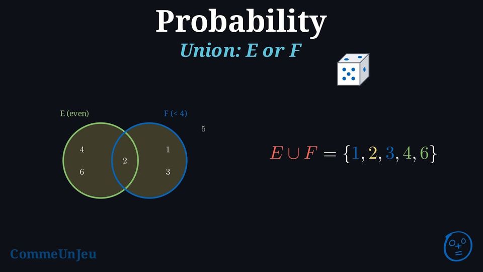
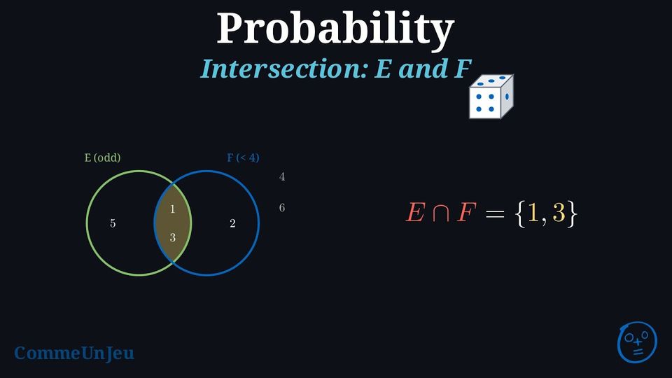
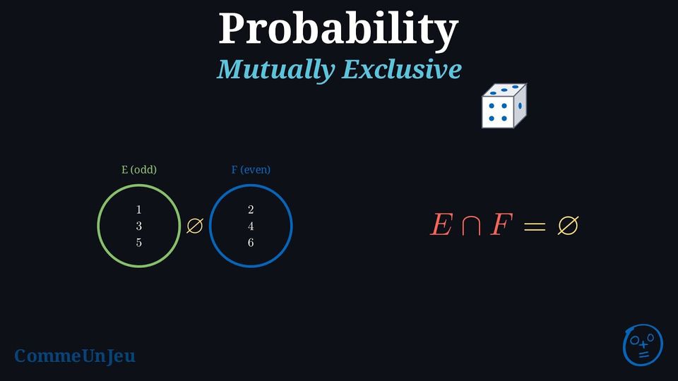
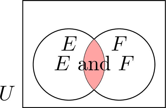
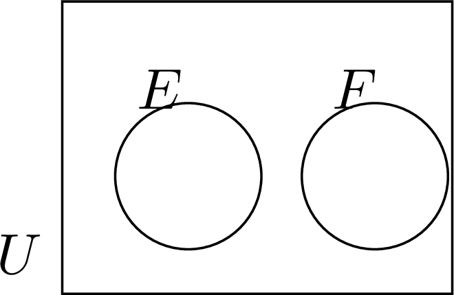
Concrete. One die, two sentences: “even” and “more than \(4\)”. Ask for the faces that make “even or more than \(4\)” happen, then “even and more than \(4\)”. The PYP hoops come back with their names. Pictorial. The union \(E \cup F\) (“\(E\) or \(F\)”, possibly both), the intersection \(E \cap F\) (“\(E\) and \(F\)”), and two mutually exclusive events, \(E \cap F = \emptyset\). 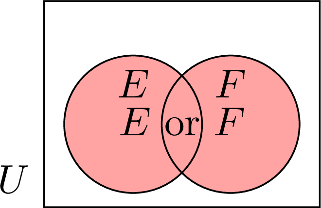
A two-step experiment has pairs for outcomes: for “a coin then a die”, \(2 \times 6 = 12\) pairs, and “heads and even” is a set of \(3\) of them. 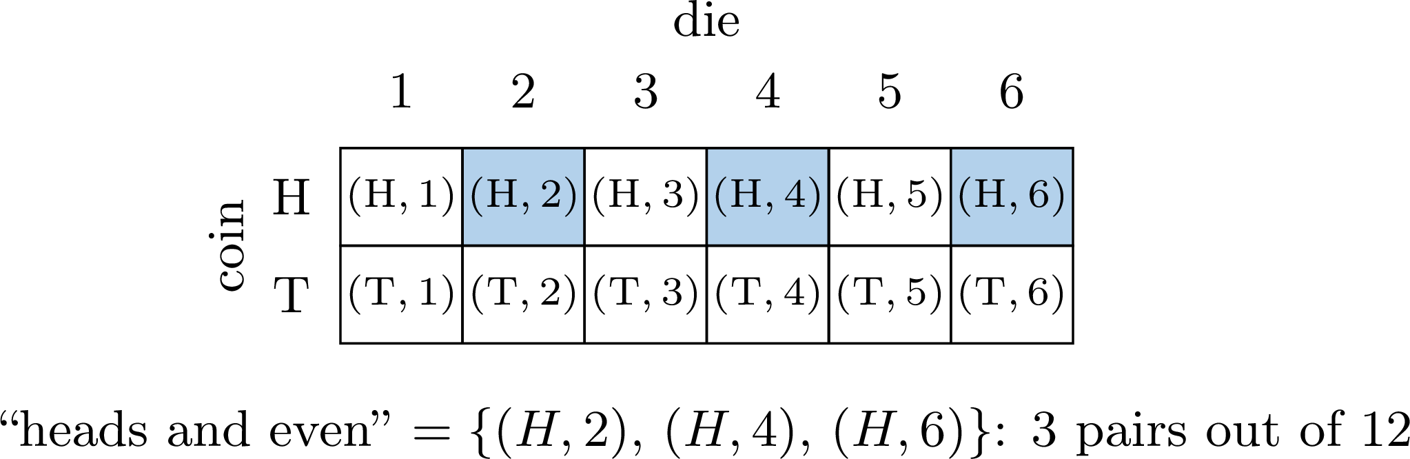
Abstract. The method of every calculation has two steps: determine the event (describe it, list its outcomes, write it as a set), then compute its probability, by counting if the outcomes are equally likely, by adding the probabilities of its outcomes otherwise, or through the complement when it is simpler. Two remarks, in MYP 5, prevent two confusions: mutually exclusive does not mean complementary, and the probabilities of two mutually exclusive events need not add up to \(1\). Where to find it. MYP 3, Probability: Events and Their Probabilities (Events as Sets, Listing the Outcomes in a Table, The Probability of an Event, The Complement Rule, Probabilities from a Venn Diagram), then Two-Step Experiments (Independent Events). MYP 4, Events and Venn Diagrams (Events in the Language of Sets).
The Addition Relation, and d'Alembert's Two Tosses (MYP 4 and MYP 5)
Concrete. A school chooses one student at random for a talent show: the outcomes are the students. \(40\pourcent\) sing, \(30\pourcent\) dance, \(10\pourcent\) do both. What is the probability that the student chosen sings or dances? Pictorial. Fill the Venn diagram from the middle: \(0.1\) in both, so \(0.3\) sing only and \(0.2\) dance only. 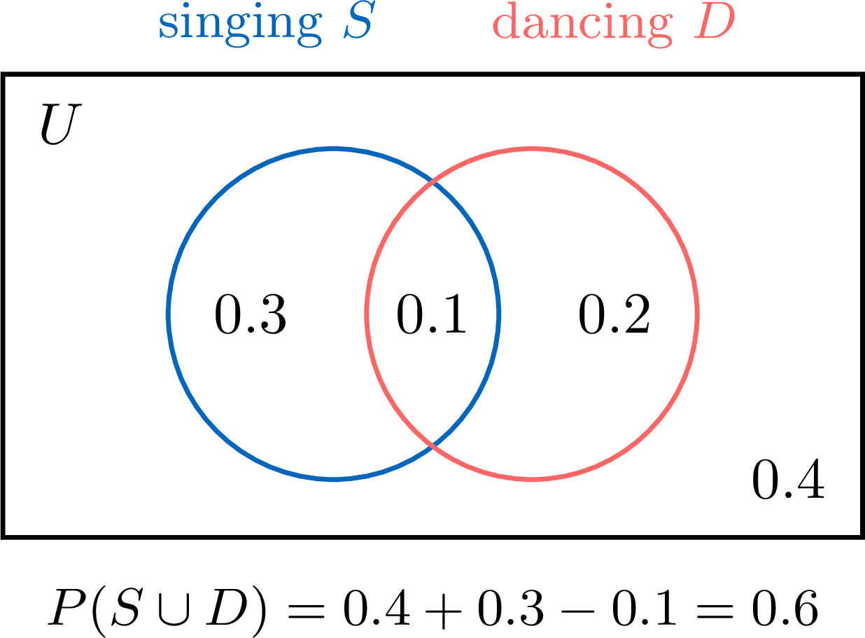
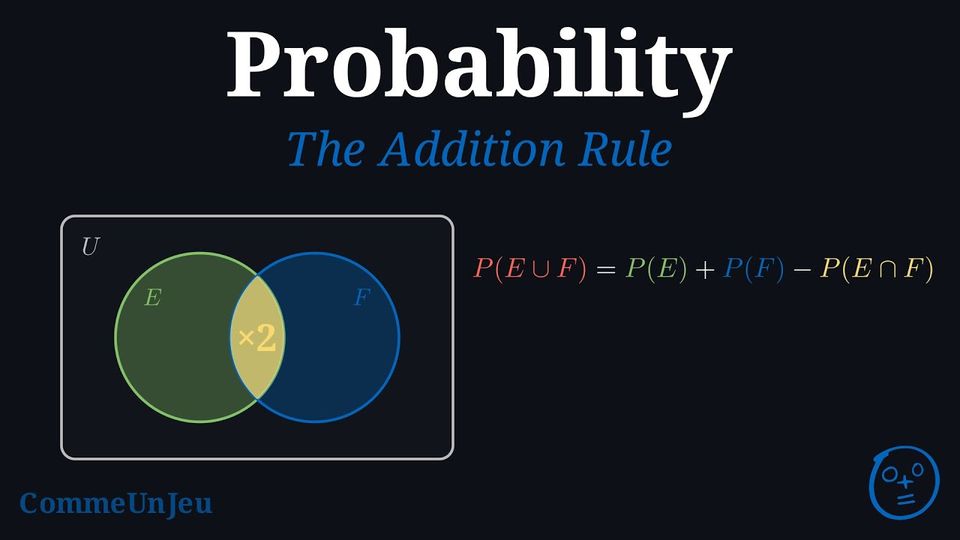
The outcomes of \(E \cap F\) are in \(E\) and in \(F\): in \(P(E) + P(F)\) they are counted twice. 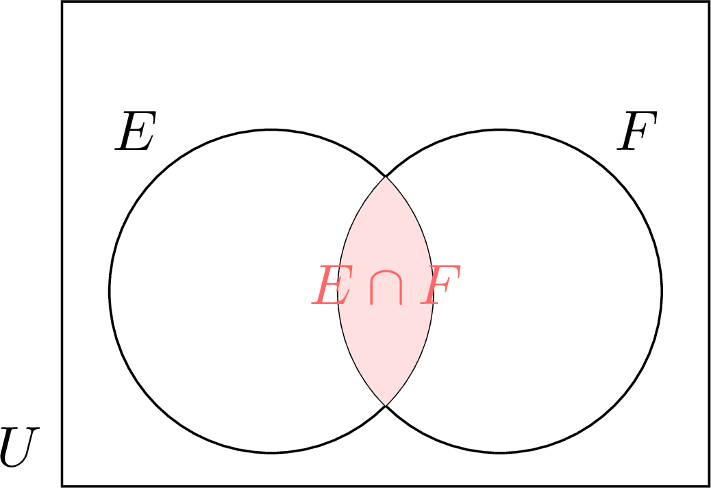
Abstract. \(P(E \cup F) + P(E \cap F) = P(E) + P(F)\), a balance between four numbers: three of them give the fourth. MYP 5 proves it, with the drawing and then with events, before using it. A problem from history. In 1754, d'Alembert disputed the usual answer to “heads at least once in two tosses”. His three cases—heads at the first toss, tails then heads, tails then tails—are not equally likely: the first one gathers two outcomes of the four. 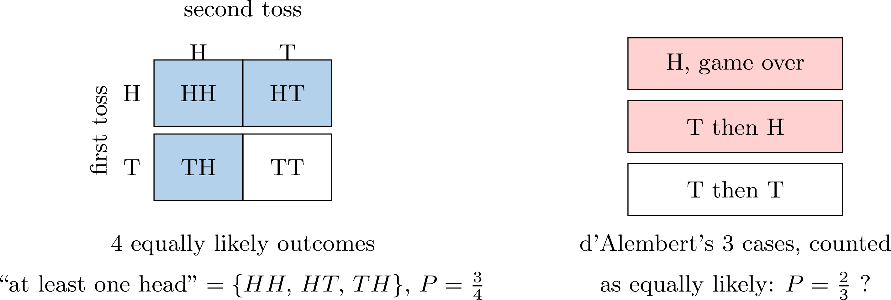
Where to find it. MYP 4, Probability: Events and Venn Diagrams, and in Going further, Solving Historical Problems of Chance (d'Alembert). MYP 5, Probability: The Complement Rule and the Addition Law.
Sets and Events in One Table; the Axioms and the Rules (MYP 5)
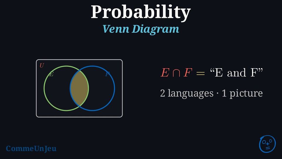
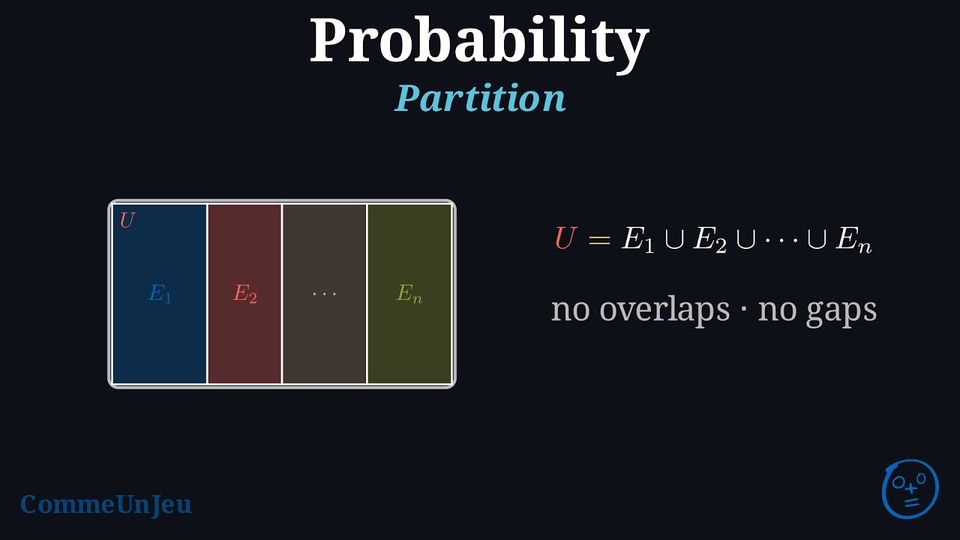
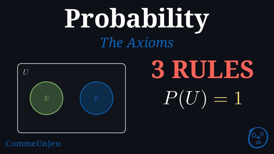
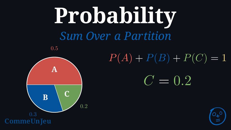
Pictorial. One table translates every word: the notation, the word of set theory, the word of probability, the Venn diagram. Project it all year.
A partition of the sample space: events that never overlap and together cover \(U\). 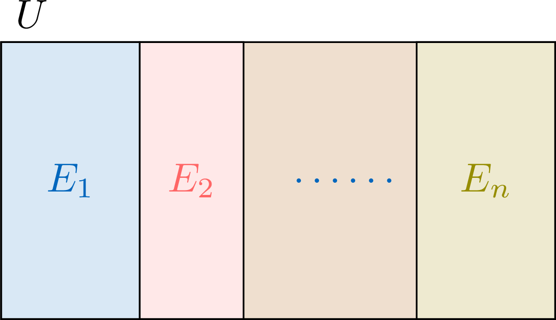
Abstract. MYP 5 follows the order of this guide: The Algebra of Events, then The Axioms of Probability, then The Rules, Carried Over from the Events. The three axioms say what a probability must do with the events: never negative, \(1\) for the whole sample space, and additive for mutually exclusive events. 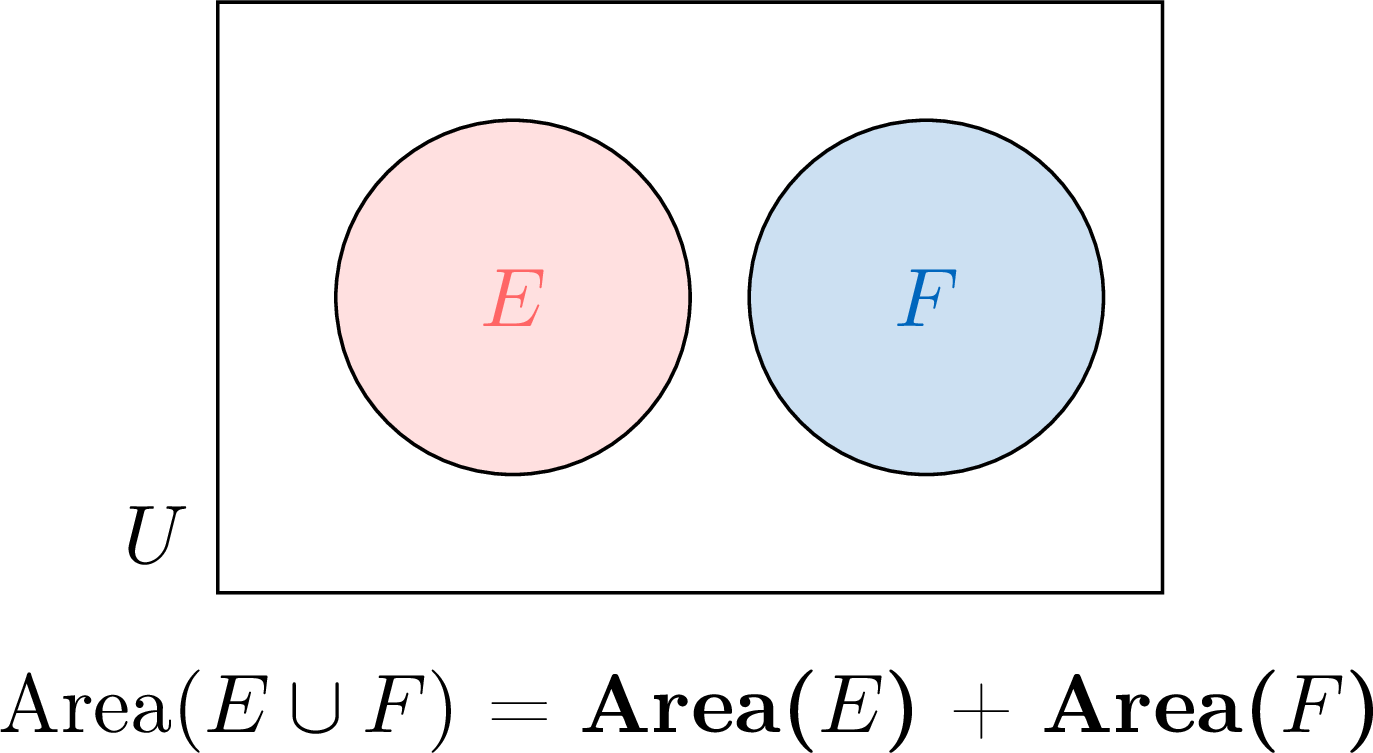
Every rule then follows from the events. If \(A \subseteq B\), the outcomes of \(A\) are among those of \(B\): \(P(A) \leq P(B)\). 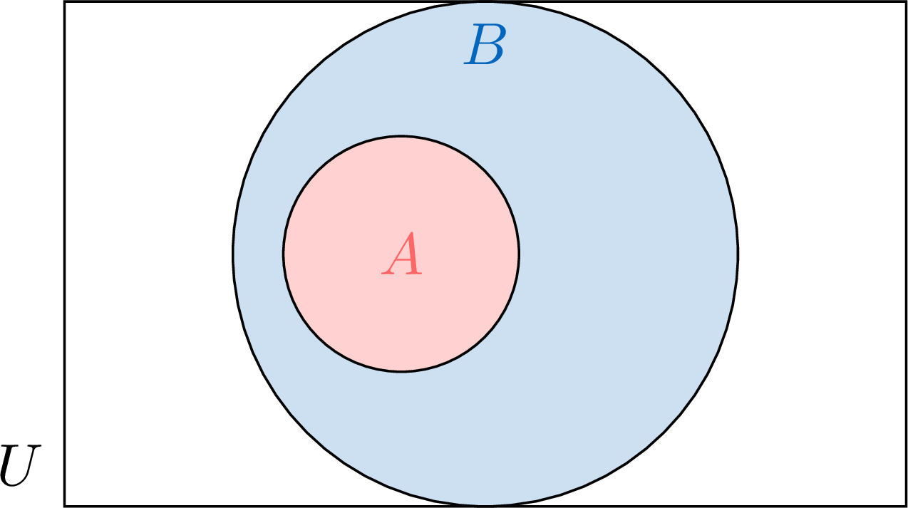
The complement rule comes from the partition into \(E\) and \(E'\), and the equally likely formula itself is proved from the axioms. 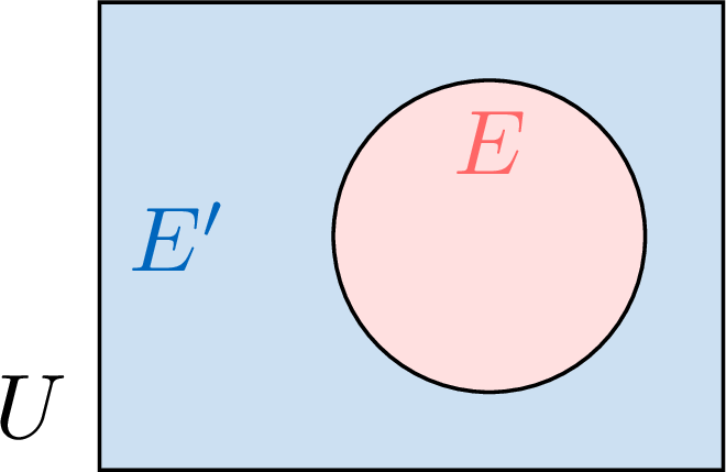
Where to find it. MYP 5, Probability: The Algebra of Events (Events in the Language of Sets, Mutually Exclusive Events, Partitions of the Sample Space), The Axioms of Probability, The Rules, Carried Over from the Events. The DP 1 chapter Probability opens the same way, with The World of Events.
| Notation | Set Vocabulary | Probability Vocabulary | Venn Diagram |
| \(U\) | Universal set | Sample space | 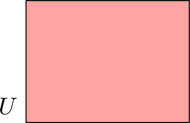 |
| \(x\) | Element of \(U\) | Outcome | 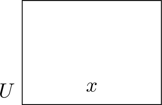 |
| \(\emptyset\) | Empty set | Impossible event | |
| \(E\) | Subset of \(U\) | Event | 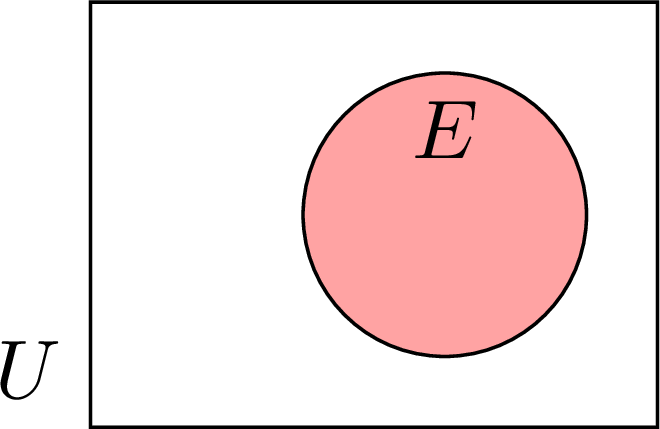 |
| \(x \in E\) | \(x\) is an element of \(E\) | \(x\) is an outcome of \(E\) | 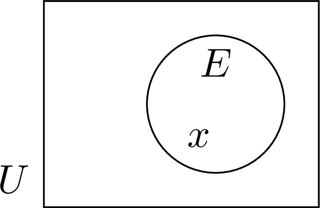 |
| \(E'\) | Complement of \(E\) in \(U\) | Complementary event of \(E\) | 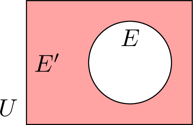 |
| \(E \cup F\) | Union of \(E\) and \(F\) | \(E\) or \(F\) | |
| \(E \cap F\) | Intersection of \(E\) and \(F\) | \(E\) and \(F\) | |
| \(E \cap F = \emptyset\) | \(E\) and \(F\) are disjoint | \(E\) and \(F\) are mutually exclusive | |
Conditional Probability: Same Events, a New Measure (MYP 5 and DP 1)
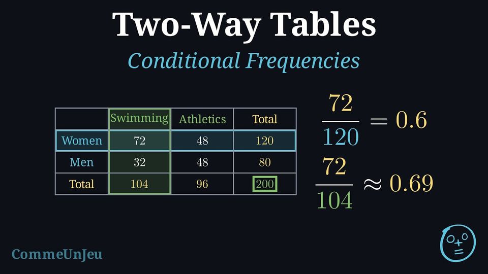
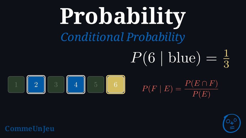
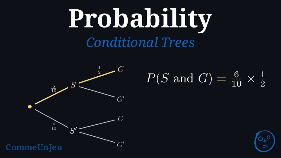
Concrete. The \(600\) pupils of a school, sorted by age and by lunch arrangement. A pupil is chosen at random.
Pictorial. “Given that the pupil is under \(16\)” keeps the same pupils and the same events; only the numbers attached to them change. The new probability gives \(1\) to the known event, \(0\) to the outcomes outside it, and is rescaled inside. 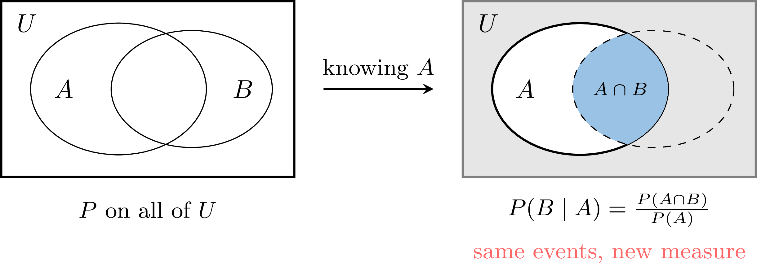
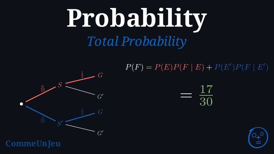
Abstract. \(P(F \mid E) = \dfrac{P(E \cap F)}{P(E)}\), with \(P(E) > 0\). A weighted tree carries the conditional probabilities on its branches; the product along a path gives the probability of the intersection. 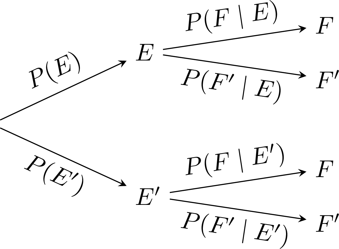
MYP 5 and DP 1 state the second reading as a proposition, Conditioning Changes the Probability, Not the Events, with its proof: \(F \mapsto P(F \mid E)\) is a probability on the same sample space, so every rule holds for it. When \(P(E) > 0\) and \(P(F) > 0\), \(P(E \mid F)\) and \(P(F \mid E)\) have the same numerator, \(P(E \cap F)\), and the denominators \(P(F)\) and \(P(E)\), which need not be equal: the screening test of the errors section shows why the difference matters. Where to find it. MYP 5, Conditional Probability: Two-Way Tables and Conditional Frequencies, Conditional Probability (Probability Given an Event), Tree Diagrams, with the exercises Inverting the Conditioning: False Positives. DP 1, Conditional Probability, in the four courses.
| Eats at school | Eats elsewhere | Total | |
| Under 16 | \(180\) | \(60\) | \(240\) |
| 16 or over | \(210\) | \(150\) | \(360\) |
| Total | \(390\) | \(210\) | \(600\) |
Frequencies at the End of the Chapter: Trials, Fluctuation, Simulation (PYP 3 to MYP 4)
From PYP 3 on, when a chapter has repeated trials, they close the chapter. They come after the probability has been built, and they serve the two purposes of the third gesture: estimate a probability, test a model. PYP 3 to PYP 5: predict, then try. Before the trials, the pupil predicts from the outcomes: \(30\) rolls of a fair die, about \(5\) of each face. Then the tally, and the comparison: the totals are close to the prediction without being equal to it, and another series gives other totals.
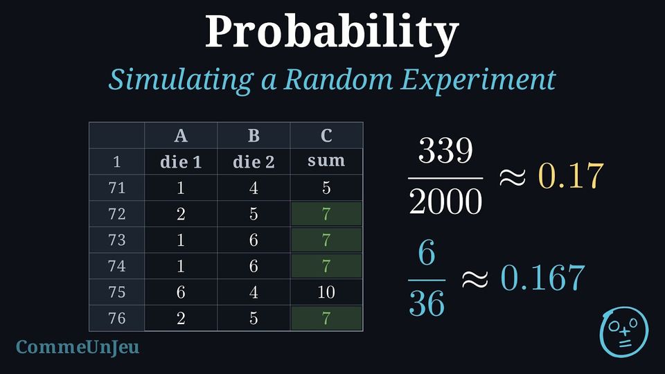
MYP 2 to MYP 4: the frequency. The frequency of an event is its count divided by the number of trials. It fluctuates from one series to another, and long series usually stray less from the probability than short ones. A simulation replaces a slow experiment by a quick one with the same probabilities: a spreadsheet rolls two dice \(2\,000\) times and finds \(339\) sums of \(7\), a frequency close to the exact \(\dfrac{6}{36}\) read in the table of the \(36\) outcomes.
Abstract. The frequency estimates a probability; it never defines it. Write \(f \approx P\), and keep the letter \(P\) for the model. Where to find it. PYP 3, Carrying Out Chance Experiments (Predicting the Results of an Experiment, Counting the Results of an Experiment, Doing an Experiment and Comparing). PYP 4, Chance Experiments (Comparing Results with the Probability). PYP 5, Experimental Probability. MYP 2, Experimental Probability. MYP 3, Experimental Probability and Expected Counts. MYP 4, Expected Gain, Fair Games and Simulation. DP 1, Probability: Relative Frequency and Predictions.
| Face | Tally Marks | Total |
| \(1\) |  | 4 |
| \(2\) | 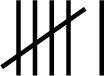 | 6 |
| \(3\) |  | 5 |
| \(4\) |  | 3 |
| \(5\) | 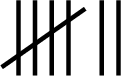 | 7 |
| \(6\) | | 5 |
| \(+\) | \(1\) | \(2\) | \(3\) | \(4\) | \(5\) | \(6\) |
| \(1\) | \(2\) | \(3\) | \(4\) | \(5\) | \(6\) | \(7\) |
| \(2\) | \(3\) | \(4\) | \(5\) | \(6\) | \(7\) | \(8\) |
| \(3\) | \(4\) | \(5\) | \(6\) | \(7\) | \(8\) | \(9\) |
| \(4\) | \(5\) | \(6\) | \(7\) | \(8\) | \(9\) | \(10\) |
| \(5\) | \(6\) | \(7\) | \(8\) | \(9\) | \(10\) | \(11\) |
| \(6\) | \(7\) | \(8\) | \(9\) | \(10\) | \(11\) | \(12\) |
Random Variables and Repeated Trials, Briefly (DP 1 and DP 2)
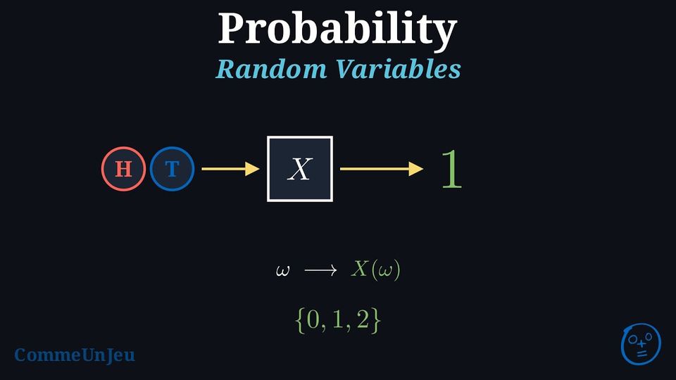
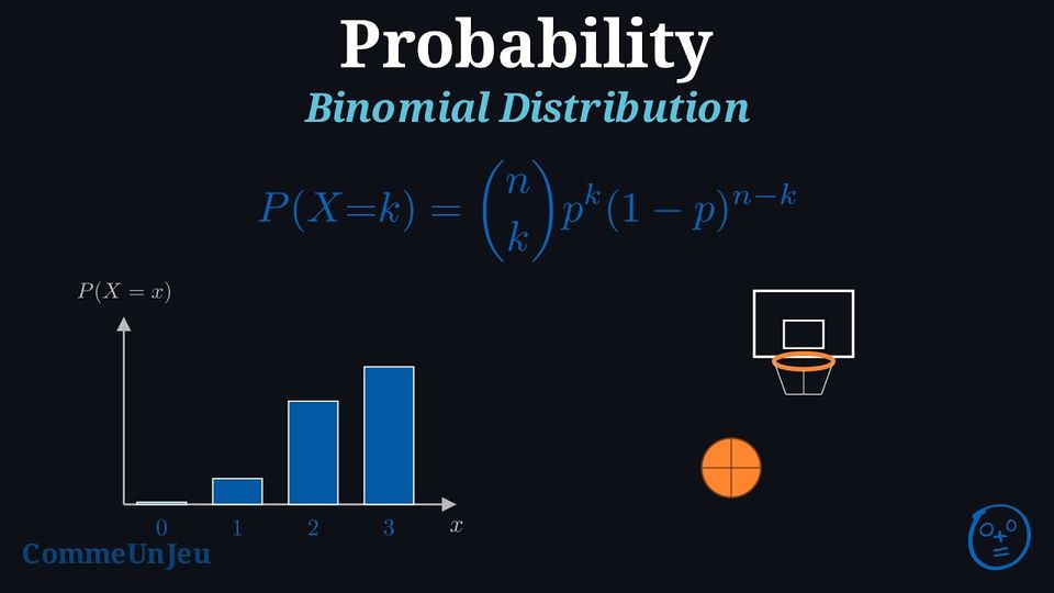
The same separation, one level up. A random variable is a function on the sample space before it has a distribution: \(X\), the number of heads in two independent tosses of a fair coin, sends each outcome to a number, and \((X = 1)\) is an event, the set of the outcomes where \(X\) takes the value \(1\). 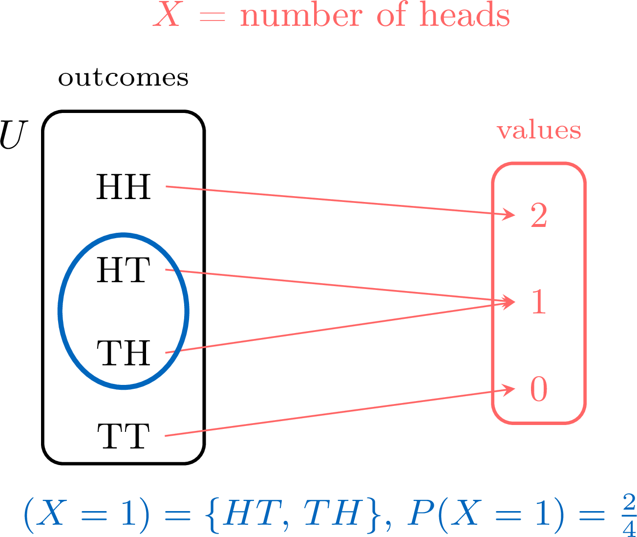
Its distribution is the probability applied to these events: \(P(X = 1) = P(\{HT, TH\}) = \dfrac{2}{4}\). In a Bernoulli scheme with \(n\) trials, let \(X\) count the successes: the binomial coefficient \(\binom{n}{k}\) counts the paths of the tree in the event \((X = k)\). 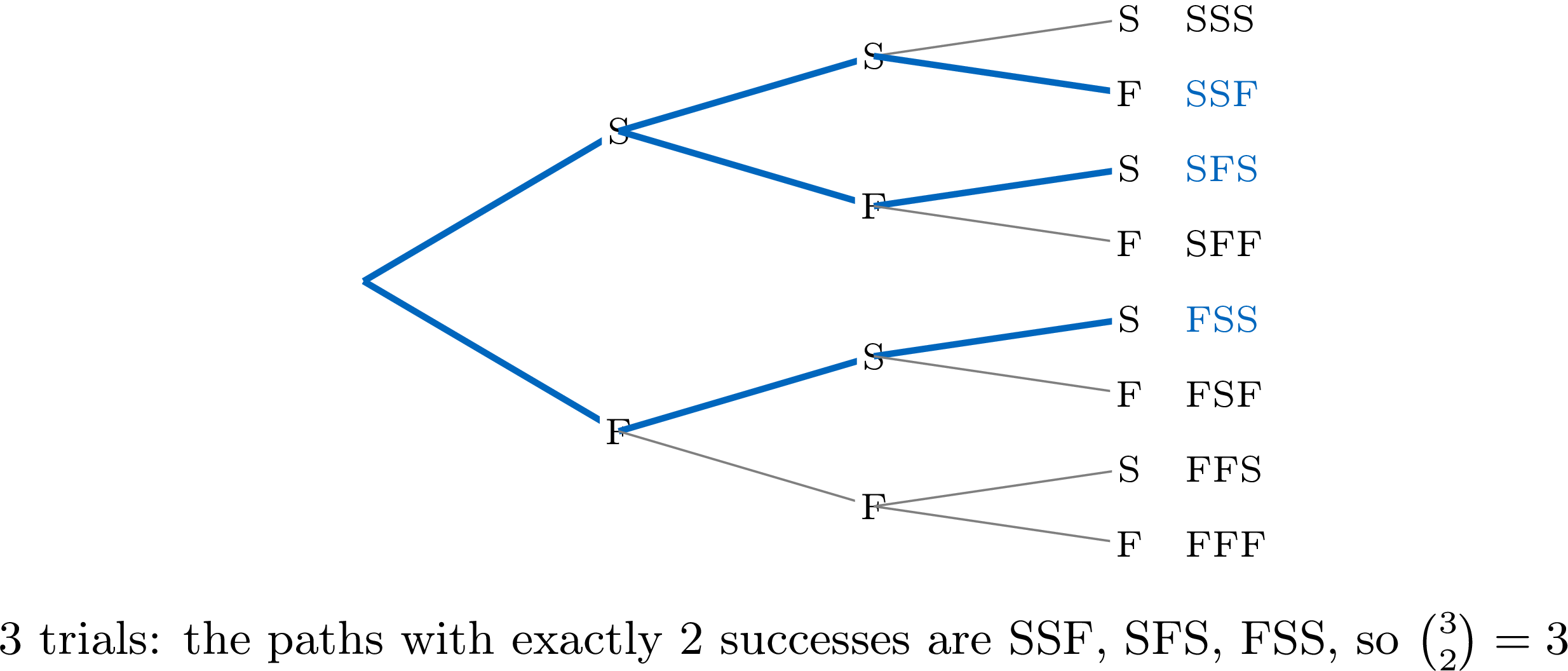
With replacement, the same urn gives the same branches at the second draw: the trials are independent, and the product of the branches gives the probability of a path. 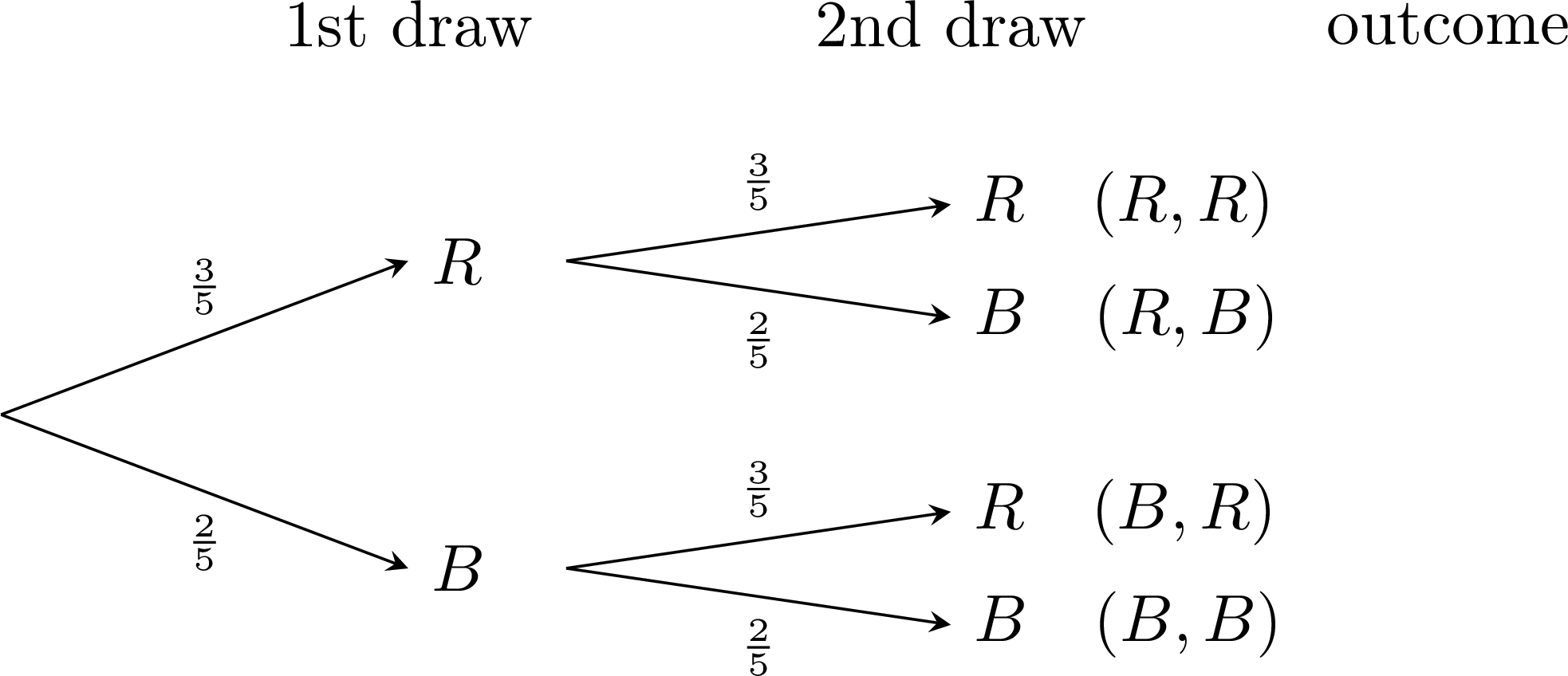
Where to find it. DP 1, Probability (Independent Events, at the end of Probability). DP 2, Discrete Random Variables: Random Variables, Expected Value, Repeated Trials, The Bernoulli and Binomial Distributions.
Errors to Watch For, and the Figure That Answers Each
Most of these errors are not about numbers: they come from an event that was never built, or from outcomes counted as if they were equally likely. For each one, a figure gives the answer; the pupil draws it, and the error shows.
- “The event is \(\dfrac{1}{6}\).” Three objects, three names: the face \(3\) is an outcome, \(\{3\}\) is an event, \(\dfrac{1}{6}\) is its probability (MYP 2, Singleton Events; MYP 5, An Event Is a Set and a Probability Is a Number).
- “Two possible results, so one chance in two.” On spinner A the pointer stops on red or not red, two results, yet red is \(2\) of the \(6\) equal parts: \(\dfrac{2}{6}\), not \(\dfrac{1}{2}\). Count equal parts, not results (PYP 3, Probability, a Number from 0 to 1).
- “Three colours, so \(P(\text{red}) = \dfrac{1}{3}\).” The colours are outcomes, but not equally likely ones. To calculate by counting, take the counters as the outcomes (PYP 3, Recognising Equally Likely Outcomes).
- “Three sixes in a row: the next one cannot be a six”, or “the die is lucky today”. Nothing has changed between the rolls; the chances have not changed either (PYP 5, the remark that opens Experimental Probability).
- “Heads at least once in two tosses: \(\dfrac{2}{3}\).” D'Alembert's three cases are not equally likely. Draw the table of the four ordered outcomes (MYP 4, Solving Historical Problems of Chance).
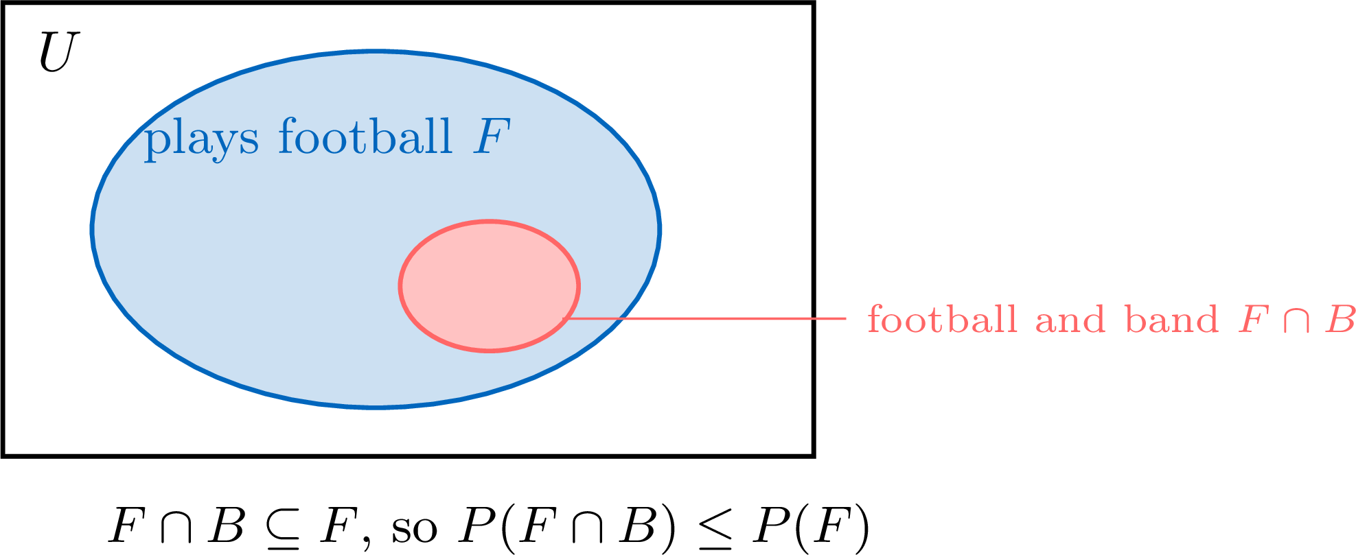
- “Plays football and is in the band” judged more likely than “plays football”. The pupils who do both are among those who play football: \(F \cap B \subseteq F\), so \(P(F \cap B) \leq P(F)\) (MYP 5, the rule \(A \subseteq B \Rightarrow P(A) \leq P(B)\)).
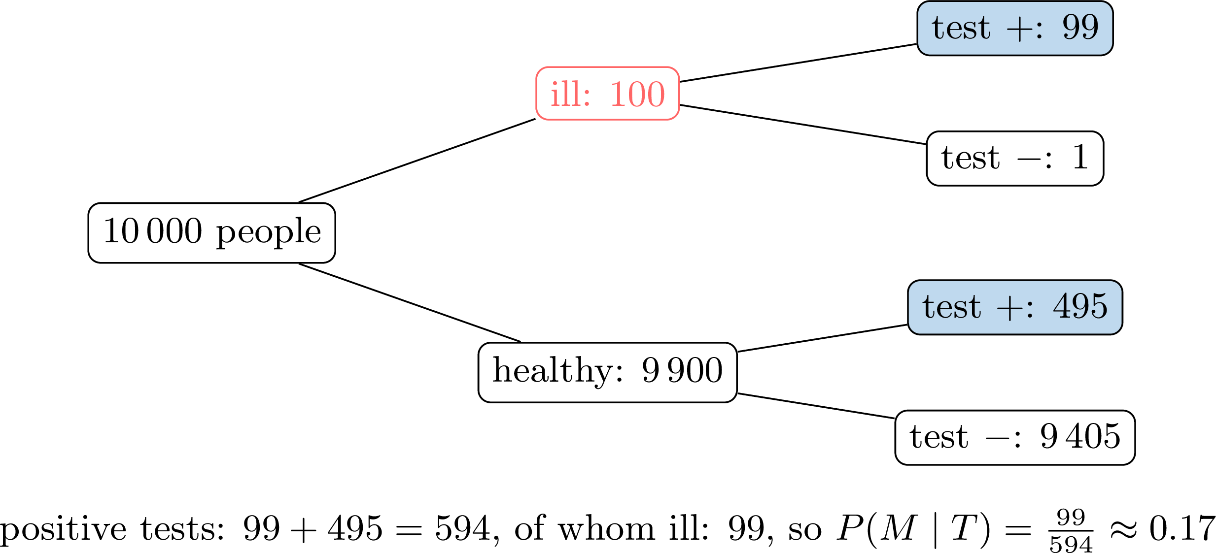
- “The test is positive for \(99\pourcent\) of ill people, so a positive person is ill with probability \(0.99\).” \(P(T \mid M)\) and \(P(M \mid T)\) are different numbers. Follow \(10\,000\) people through the tree: of \(594\) positive tests, only \(99\) are ill (MYP 5, Inverting the Conditioning: False Positives).
- “No six in twelve rolls: the die is loaded”, or “\(\dfrac{15}{50}\) is the probability”. A frequency fluctuates; it estimates the probability, it is not it. Twelve rolls are few; over hundreds of independent rolls, the frequency is usually close to the probability (MYP 2, Experimental Probability, method Comparing a Series of Trials to the Calculated Probability).
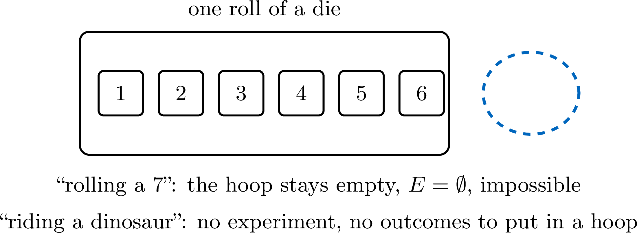
- “Riding a dinosaur is impossible” given as an example of an event. An event belongs to an experiment. In one roll of a die, “rolling a \(7\)” is impossible because its hoop is empty; the dinosaur has no experiment and no outcomes (PYP 3, the probability line).
- “Mutually exclusive, so complementary.” Two events with no outcome in common need not cover the sample space, and their probabilities need not add up to \(1\) (MYP 5, the two remarks after the complement rule).
One Task Taken Apart: the Two Hoops
The task: a tray of counters that all have the same chance of being picked, and two sentences about the counter picked. The pupil puts in hoop \(A\) the counters that make the first sentence true, in hoop \(B\) those of the second, then answers: which counters make “not \(A\)”, “\(A\) and \(B\)”, “\(A\) or \(B\)” happen? Certain, possible or impossible? No number is needed. The same task can be easy or hard; to adapt it in class, vary these five settings one at a time. 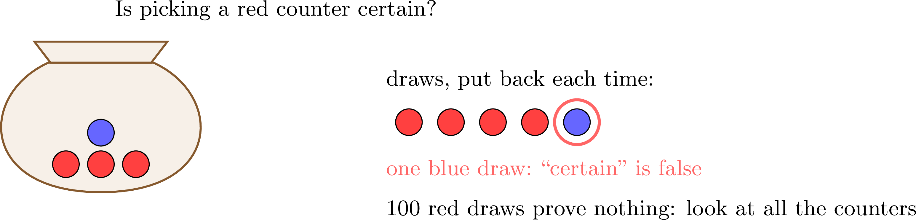
To find out where a pupil stands, give crossing hoops on counters with two attributes and ask for “red or round”. The pupil who leaves out the red round counters reads “or” as “one or the other, not both”. Where to find it. PYP 2, Not, Or, And, with the exercises Finding the Counters That Are Not… and Using Two Hoops; the hoop of one sentence comes from PYP 0 and PYP 1 (Filling the Hoop).
- The number of counters, from four to eight.
- One attribute or two. Colour and shape give two simple criteria whose events can cross without either containing the other.
- How the events are given: by a sentence, by a list, or by a hoop already filled.
- How the hoops meet: disjoint, nested, crossing.
- The symmetry: counters alike apart from colour and shape, so that later the counts can become probabilities.
In Class
- Ask “which outcomes?” before “how likely?”. Write the hoop, the list or the set on the board before any number, and require it on paper.
- Check that the outcomes are equally likely before counting: counters alike, a spinner with equal parts. Numbering the counters, or writing the ordered pairs, tells the outcomes apart; the equal chances come from the experiment.
- Keep the two objects apart in writing. \(E = \{2, 4, 6\}\) and \(P(E) = \dfrac{1}{2}\): an event equals a set, a probability equals a number. Correct \(E = \dfrac{1}{2}\) every time it appears.
- Draw before the formula. The complement rule and the addition relation are read on the hoops before they are written.
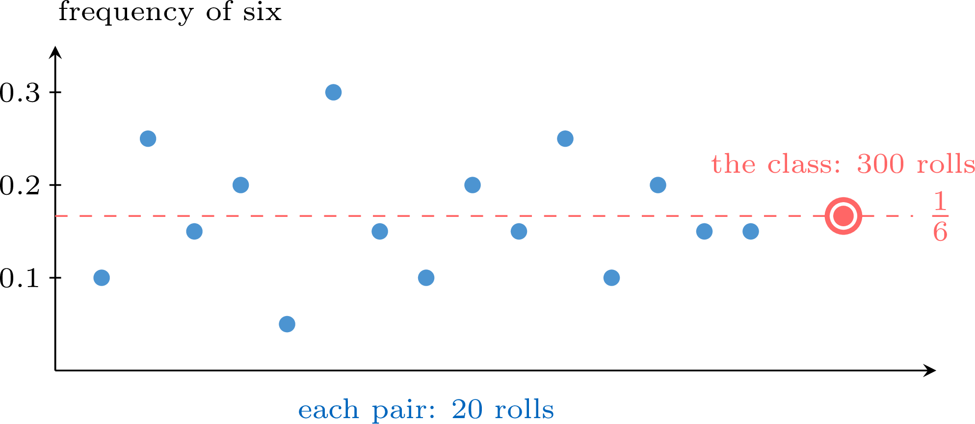
- Put the trials at the end of the chapter, and pool them. Predict from the model first; then each pair rolls \(20\) times and the class adds up its results. The pairs' frequencies scatter; the frequency calculated over the class's \(300\) rolls is usually close to the probability. Say “frequency”, write \(f \approx P\).
- One task to find out where a pupil stands. A bag holds \(3\) red counters and \(2\) blue counters. (a) Put in the hoop the counters that make “red” happen. (b) Is picking a red counter certain, possible or impossible? (c) From PYP 3: what is its probability? Three answers: a set, a word, a number. A pupil who writes \(\dfrac{3}{5}\) in the hoop, or “the red counters” as the probability, has merged the two objects.
Going Further
The choices described here (the event before its probability, circling before counting, frequencies last) are analysed in a research article, in English, which also says where the chapters still fall short of them: An event is a set, not a number.