International Baccalaureate · MYP 3
Probability
I
Events and Their Probabilities
I.1
Events as Sets
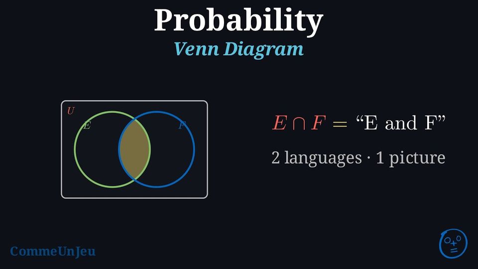
Definition — Set Theory and Probability Vocabulary
| Notation | Set Vocabulary | Probability Vocabulary | Venn Diagram |
| \(U\) | Universal set | Sample space | 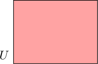 |
| \(x\) | Element of \(U\) | Outcome | 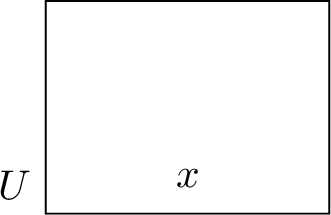 |
| \(\emptyset\) | Empty set | Impossible event | |
| \(E\) | Subset of \(U\) | Event | 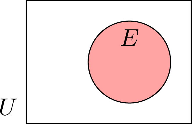 |
| \(x \in E\) | \(x\) is an element of \(E\) | \(x\) is an outcome of \(E\) | 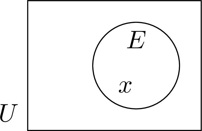 |
| \(E'\) | Complement of \(E\) in \(U\) | Complementary event of \(E\) | 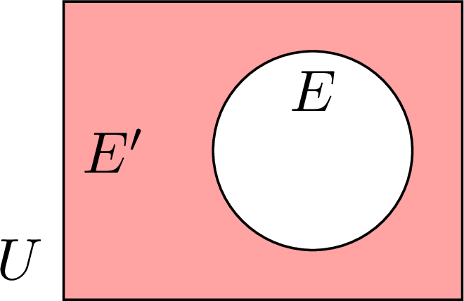 |
| \(E \cup F\) | Union of \(E\) and \(F\) | \(E\) or \(F\) | 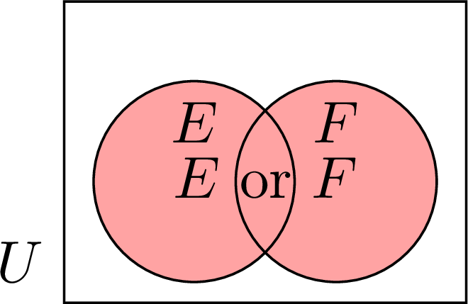 |
| \(E \cap F\) | Intersection of \(E\) and \(F\) | \(E\) and \(F\) | 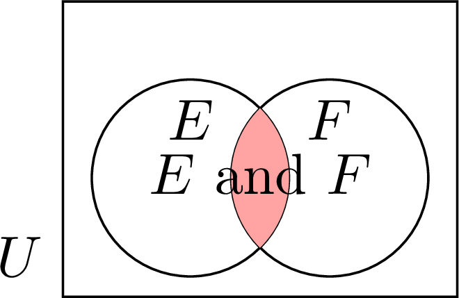 |
| \(E \cap F = \emptyset\) | \(E\) and \(F\) are disjoint | \(E\) and \(F\) are mutually exclusive | 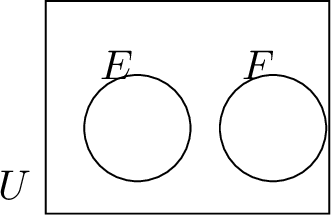 |
Example
One die is rolled: \(U = \{1, 2, 3, 4, 5, 6\}\). Consider the events \(E\): “the result is even” and \(F\): “the result is at least five”. Using the language of sets: - Is \(4 \in E\)? Is \(4 \in F\)?
- Write \(E \cup F\), \(E \cap F\) and \(E'\).
- Are \(E\) and \(F\) mutually exclusive?
Here \(E = \{2, 4, 6\}\) and \(F = \{5, 6\}\).
- \(4\) is even, so \(4 \in E\); but \(4 < 5\), so \(4 \notin F\).
- \(E \cup F = \{2, 4, 5, 6\}\) (in \(E\) or in \(F\)); \(E \cap F = \{6\}\) (in both); \(E' = \{1, 3, 5\}\) (everything else in \(U\)).
- \(E \cap F = \{6\} \neq \varnothing\): the outcome \(6\) realises both events, so \(E\) and \(F\) are not mutually exclusive.
Skills to practice
- Finding the Union and the Intersection of Two Events
I.2
Listing the Outcomes in a Table
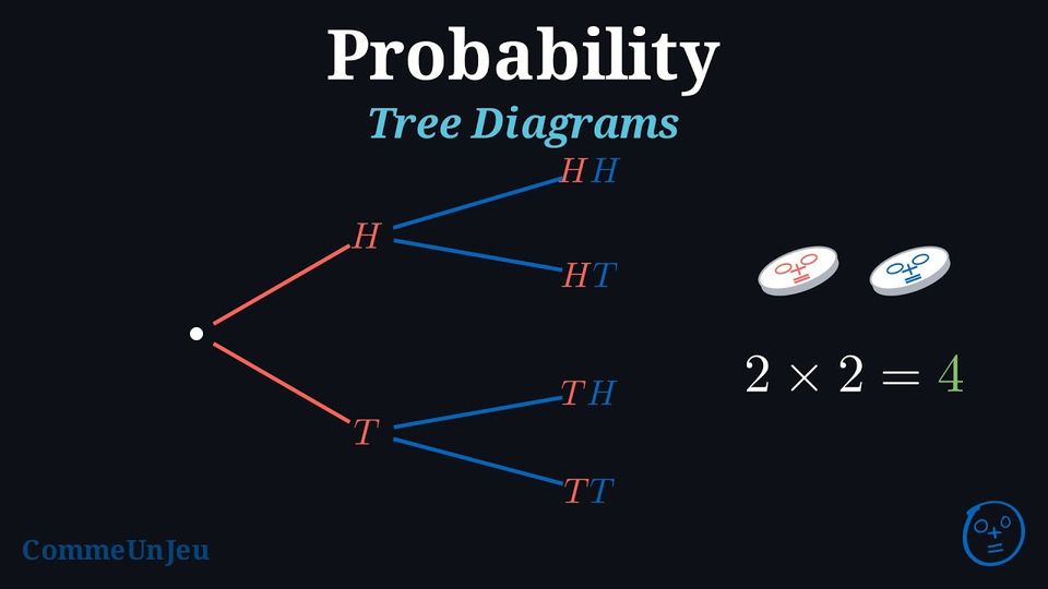
A multi-step experiment is a random experiment made up of a sequence of two or more simple steps. For example, flipping two coins is a multi-step experiment composed of two actions: flipping the first coin and then flipping the second.
In many multi-step experiments, we can find the total number of possible outcomes by multiplying the number of outcomes at each step. To display all the combined outcomes, we can use tools like lists, tables, or tree diagrams.
In many multi-step experiments, we can find the total number of possible outcomes by multiplying the number of outcomes at each step. To display all the combined outcomes, we can use tools like lists, tables, or tree diagrams.
Method — Representing Sample Spaces for Multi-Step Experiments
When an experiment has more than one step, the sample space can be represented in several ways: - by listing all possible ordered outcomes;
- using a table (best for two-step experiments);
- using a tree diagram (useful for any number of steps).
Example
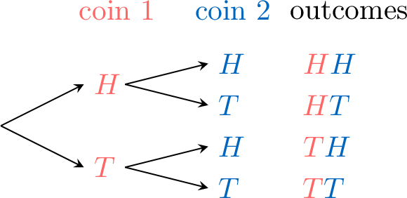
For the experiment of tossing two coins, represent the sample space by: - listing all possible outcomes;
- using a table;
- using a tree diagram.
- List:
Each outcome records the result of coin 1 first, then coin 2: $$\{\textcolor{colordef}{H}\textcolor{colorprop}{H}, \textcolor{colordef}{H}\textcolor{colorprop}{T}, \textcolor{colordef}{T}\textcolor{colorprop}{H}, \textcolor{colordef}{T}\textcolor{colorprop}{T}\}$$ - Table:
\(\begin{aligned} & \textcolor{colorprop}{\text{coin 2}} \\ \textcolor{colordef}{\text{coin 1}} \end{aligned} \) \(\textcolor{colorprop}{H}\) \(\textcolor{colorprop}{T}\) \(\textcolor{colordef}{H}\) \(\textcolor{colordef}{H}\textcolor{colorprop}{H}\) \(\textcolor{colordef}{H}\textcolor{colorprop}{T}\) \(\textcolor{colordef}{T}\) \(\textcolor{colordef}{T}\textcolor{colorprop}{H}\) \(\textcolor{colordef}{T}\textcolor{colorprop}{T}\) - Tree diagram:
Definition — Sample Space of a Two-Step Experiment
The outcomes of a two-step experiment are pairs: a result for the first step, then a result for the second. The sample space is the set of all these pairs. The table shows them all: one row per first-step outcome, one column per second-step outcome. So the number of pairs is the number of first-step outcomes times the number of second-step outcomes. (This counts every pair only when each second-step result can still occur after the first step; if an earlier result rules some out, only the remaining pairs form the sample space.) Example
For the game “a coin then a die”, list all the outcomes of the sample space, and give their number.
The first step (the coin) has \(2\) outcomes and the second (the die) has \(6\). The sample space is the set of all pairs, which the table lists in full:
There are \(2 \times 6 = 12\) outcomes, for instance \(\textcolor{colordef}{H}\textcolor{colorprop}{4}\): heads, then a \(4\).
| \(\begin{aligned} & \textcolor{colorprop}{\text{die}} \\ \textcolor{colordef}{\text{coin}} \end{aligned}\) | \(\textcolor{colorprop}{1}\) | \(\textcolor{colorprop}{2}\) | \(\textcolor{colorprop}{3}\) | \(\textcolor{colorprop}{4}\) | \(\textcolor{colorprop}{5}\) | \(\textcolor{colorprop}{6}\) |
| \(\textcolor{colordef}{H}\) | \(\textcolor{colordef}{H}\textcolor{colorprop}{1}\) | \(\textcolor{colordef}{H}\textcolor{colorprop}{2}\) | \(\textcolor{colordef}{H}\textcolor{colorprop}{3}\) | \(\textcolor{colordef}{H}\textcolor{colorprop}{4}\) | \(\textcolor{colordef}{H}\textcolor{colorprop}{5}\) | \(\textcolor{colordef}{H}\textcolor{colorprop}{6}\) |
| \(\textcolor{colordef}{T}\) | \(\textcolor{colordef}{T}\textcolor{colorprop}{1}\) | \(\textcolor{colordef}{T}\textcolor{colorprop}{2}\) | \(\textcolor{colordef}{T}\textcolor{colorprop}{3}\) | \(\textcolor{colordef}{T}\textcolor{colorprop}{4}\) | \(\textcolor{colordef}{T}\textcolor{colorprop}{5}\) | \(\textcolor{colordef}{T}\textcolor{colorprop}{6}\) |
With all the outcomes in front of us, we can describe events that combine two conditions. For two coins, take “\(E\): the first coin is heads” and “\(F\): the second coin is heads”. Then “\(E\) and \(F\)” (both happen) is the event \(\{\textcolor{colordef}{H}\textcolor{colorprop}{H}\}\), while “\(E\) or \(F\)” (at least one happens) is the event \(\{\textcolor{colordef}{H}\textcolor{colorprop}{H}, \textcolor{colordef}{H}\textcolor{colorprop}{T}, \textcolor{colordef}{T}\textcolor{colorprop}{H}\}\). Each combination is itself an event — a set of outcomes.
Skills to practice
- Finding an Outcome in a Table
- Counting the Outcomes in a Table
- Counting the Outcomes of an Event
I.3
The Probability of an Event
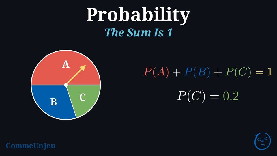
Proposition — Sum of the Probabilities
In a random experiment, the probabilities of all the outcomes add up to \(1\): $$\textcolor{colorprop}{P(\text{outcome}_1) + P(\text{outcome}_2) + \dots + P(\text{outcome}_n) = 1}$$
Probability of an Outcome
An outcome \(x\) and its singleton event \(\{x\}\) — the set with a single element — describe the same result: speaking of the chance of an outcome is therefore speaking of the chance of an event. The probability of the outcome is the probability of that event, written \(P(\{x\})\). In practice, we allow ourselves to write \(P(x)\) for \(P(\{x\})\) — for instance \(P(3)\) for the probability of rolling a 3.
Proposition — Probability of an Event
The probability of an event is the sum of the probabilities of its outcomes: $$\textcolor{colorprop}{P(\text{event}) = \text{sum of the probabilities of its outcomes}}$$
With this notation, the two rules above read: the probabilities of the outcomes \(x_1, \dots, x_n\) of \(U\) add up to \(1\), and the probability of an event \(E\) is the sum of the probabilities of the outcomes that make up \(E\). In particular, the certain event is \(U\) itself, with \(P(U) = 1\), and the impossible event is the empty set \(\emptyset\): it contains no outcome, and \(P(\emptyset) = 0\).
Definition — Equally Likely
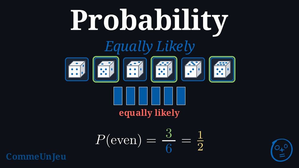
When all outcomes are equally likely, the probability of an event \(E\) is: $$\textcolor{colordef}{\begin{aligned} P(E) &= \frac{\text{number of outcomes in the event}}{\text{number of outcomes in the sample space}}\\
&=\dfrac{\Card{E}}{\Card{U}}\\
\end{aligned}}$$ Skills to practice
- Calculating the Probability of an Event
- Calculating Probabilities with a Table of Outcomes
I.4
The Complement Rule
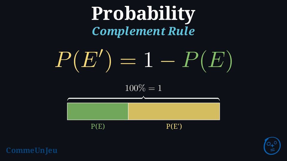
Proposition — Complement Rule
For any event \(E\) and its complementary event \(E'\), their probabilities must add up to \(1\) (or \(100\pourcent\)): $$\textcolor{colorprop}{P(E) + P(E') = 1}$$ This leads to the useful formula for finding the probability of the complement: $$\textcolor{colorprop}{P(E') = 1 - P(E)}$$
The complementary event \(E'\) is made of exactly the outcomes of \(U\) that are not in \(E\). So every outcome of \(U\) lies in exactly one of \(E\) and \(E'\): together they split \(U\) into two parts that overlap nowhere. 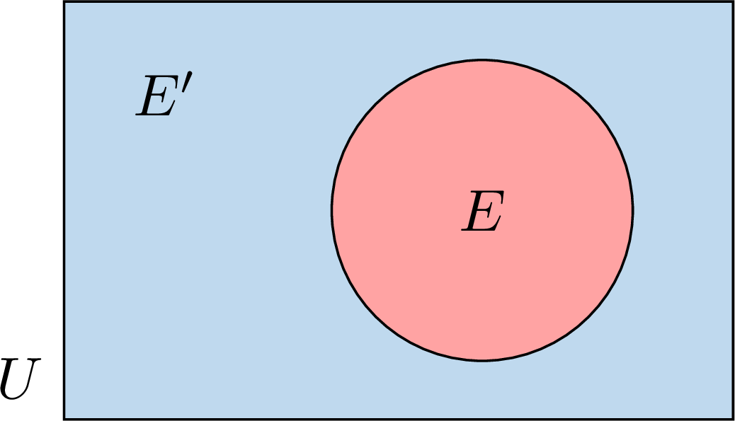
The probability of an event is the sum of the probabilities of its outcomes. Adding \(P(E)\) and \(P(E')\) therefore counts the probability of every outcome of \(U\) exactly once: $$\begin{aligned}[t] P(E) + P(E') &= \text{(sum of the probabilities of all the outcomes of } U\text{)} && \text{(every outcome is in \(E\) or in \(E'\))}\\
&= P(U) && \text{(the whole sample space)}\\
&= 1. \end{aligned}$$ Subtracting \(P(E)\) from both sides gives \(P(E') = 1 - P(E)\).
Method — Computing the Probability of an Event
- Determine the event: describe it, then list its outcomes — write it as a set.
- Compute its probability:
- if the outcomes are equally likely: \(P(A) = \dfrac{\text{number of outcomes of } A}{\text{total number of outcomes}}\);
- otherwise: add the probabilities of the outcomes of the event;
- when the complementary event is simpler: \(P(A) = 1 - P(A')\).
Skills to practice
- Applying the Complement Rule
I.5
Probabilities from a Venn Diagram
Method — Finding a Probability from a Venn Diagram
A Venn diagram gives the elements of each region, or their number written in brackets: \((9)\) is a count, a bare \(9\) is an element. The rectangle \(U\) holds the whole group of \(N\) elements. When one element of \(U\) is chosen at random, the \(N\) elements are equally likely, so $$P(\text{event}) = \frac{\text{number of elements in the regions of the event}}{N}.$$ - \(A \cap B\) (“\(A\) and \(B\)”): the overlap of the two circles;
- \(A \cup B\) (“\(A\) or \(B\)”, at least one of the two): every region inside the circles, each counted once;
- “\(A\) only”: the part of the circle \(A\) outside \(B\); “exactly one of the two”: \(A\) only and \(B\) only together;
- \(A'\) (“not \(A\)”): every region outside the circle \(A\); “neither \(A\) nor \(B\)”: the region outside both circles.
Example
In a class of \(32\) pupils, \(14\) swim (\(S\)), \(11\) run (\(R\)) and \(5\) do both. One pupil of the class is chosen at random. - Draw the Venn diagram giving the number of pupils in each region.
- Find the probability that the pupil swims, that the pupil does not swim, that the pupil does both sports, that the pupil does at least one of the two sports, and that the pupil does neither.
- Find the probability that the pupil does exactly one of the two sports.
- Swimming only: \(14 - 5 = 9\); running only: \(11 - 5 = 6\); neither: \(32 - (9 + 5 + 6) = 12\).
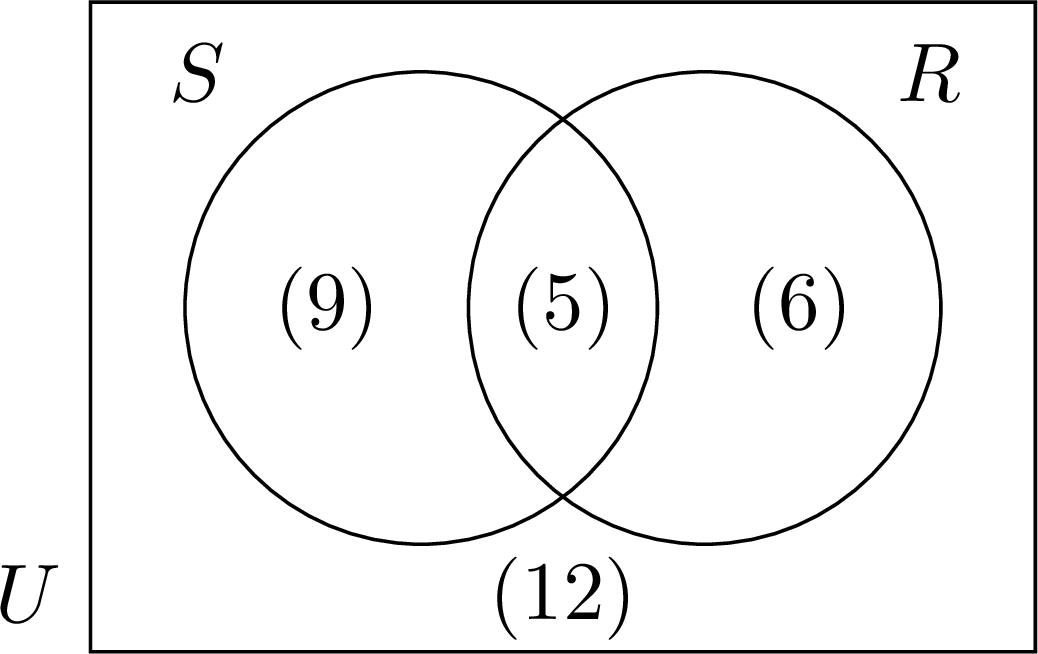
- The \(32\) pupils are equally likely to be chosen. $$\begin{aligned} P(S) &= \frac{9 + 5}{32} = \frac{14}{32} = \frac{7}{16}\\ P(S') &= \frac{6 + 12}{32} = \frac{18}{32} = \frac{9}{16}\\ P(S \cap R) &= \frac{5}{32}\\ P(S \cup R) &= \frac{9 + 5 + 6}{32} = \frac{20}{32} = \frac{5}{8}\\ P(\text{neither}) &= \frac{12}{32} = \frac{3}{8} \end{aligned}$$ “Neither” is the complementary event of “at least one”: \(\dfrac{5}{8} + \dfrac{3}{8} = 1\).
- Exactly one sport: swimming only or running only, \(9 + 6 = 15\) pupils: $$P(\text{exactly one}) = \frac{15}{32}.$$
Skills to practice
- Finding Probabilities from a Venn Diagram
II
Two-Step Experiments
II.1
Independent Events
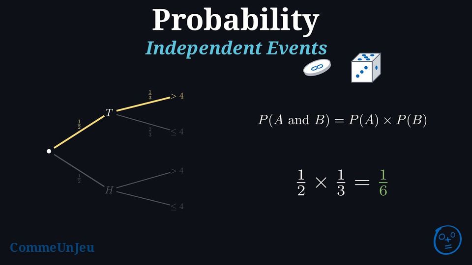
Independent events are events where knowing that one event has happened does not change the probability that the other event happens. For example, when rolling two fair dice at the same time, the result of the first die does not change the chances for the second die — they are independent events.
Definition — Independent Events
Two events \(A\) and \(B\) are independent when the probability that both happen (that is, \(P(A\cap B)\) or \(P(A \text{ and } B)\)) is the product of their individual probabilities. This is called the multiplication rule for independent events: $$P(A \text{ and } B) = P(A) \times P(B)$$ Example
An experiment consists of the following two independent actions: - Tossing a fair coin.
- Rolling a fair six-sided die.
Let \(T\) be the event “getting tails” and \(N\) be the event “rolling a number greater than 4”.
- The events are independent, so we can use the multiplication rule.
- The probability of getting tails is \(P(T) = \dfrac{1}{2}\).
- The outcomes for a number greater than 4 are \(\{5, 6\}\). There are 2 favourable outcomes out of 6 total outcomes. So, \(P(N) = \dfrac{2}{6} = \dfrac{1}{3}\).
- Now, we multiply the probabilities to find the probability of both events happening: $$\begin{aligned} P(T \text{ and } N) &= P(T) \times P(N) \\ &= \dfrac{1}{2} \times \dfrac{1}{3} \\ &= \dfrac{1}{6} \end{aligned}$$
Skills to practice
- Multiplying the Probabilities of Independent Events
III
Two-Way Tables
III.1
Two-Way Tables of Counts
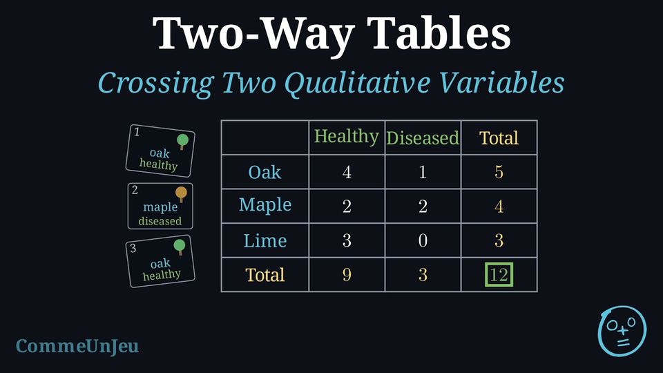
A data file describes individuals — people, animals, towns, cars — by several characteristics: species, region, profession, level of satisfaction. Crossing two of these characteristics in one table answers questions that a single list cannot: do the members of one group behave like those of another? which group holds most of a given category? A two-way table of counts is the first tool of data analysis, and reading it carefully is what keeps a sentence such as “most of the accidents with injuries happen in town” from being confused with “an accident in town is more often a serious one”.
Definition — Qualitative Variable
A qualitative variable describes the individuals of a population by a category, not by a number. Its possible values are its categories. The variable is nominal when the categories have no natural order (species, profession, region of residence) and ordinal when they do (level of education, degree of satisfaction, age group). Definition — Two-Way Table of Counts
Two qualitative variables are observed on the same population of \(N\) individuals. The two-way table of counts has one row for each category of the first variable and one column for each category of the second; the cell at row \(A\) and column \(B\) holds the count of the individuals that have both categories \(A\) and \(B\), written \(n(A \cap B)\). - The last column holds the row totals: \(n(A)\) is the number of individuals of category \(A\).
- The last row holds the column totals: \(n(B)\) is the number of individuals of category \(B\).
- The bottom-right cell holds the grand total \(N\), which is the sum of the row totals and the sum of the column totals.
Example
A gardener records the species and the state of health of the \(12\) trees of a park: | Tree | 1 | 2 | 3 | 4 | 5 | 6 |
| Species | oak | maple | oak | lime | oak | maple |
| Health | healthy | diseased | healthy | healthy | diseased | healthy |
| Tree | 7 | 8 | 9 | 10 | 11 | 12 |
| Species | lime | oak | maple | oak | lime | maple |
| Health | healthy | healthy | diseased | healthy | healthy | healthy |
Both variables are qualitative: the species (nominal, three categories) and the health (nominal, two categories). Each tree is counted in exactly one cell. The oaks are the trees \(1\), \(3\), \(5\), \(8\), \(10\): four healthy, one diseased. The maples are \(2\), \(6\), \(9\), \(12\): two and two. The limes are \(4\), \(7\), \(11\): all healthy.
Check: the row totals \(5 + 4 + 3\) and the column totals \(9 + 3\) both give the \(12\) trees.
| Healthy | Diseased | Total | |
| Oak | \(4\) | \(1\) | \(5\) |
| Maple | \(2\) | \(2\) | \(4\) |
| Lime | \(3\) | \(0\) | \(3\) |
| Total | \(9\) | \(3\) | \(12\) |
Definition — Marginal Frequency
In a two-way table with grand total \(N\), the row and column totals are the marginal counts: they are read in the margins of the table. The marginal frequency of a category \(A\) is the proportion of the whole population that has this category: $$\textcolor{colordef}{f(A) = \frac{n(A)}{N}}.$$ Here the word frequency denotes a proportion, the relative frequency; a number of individuals is a count. Likewise the frequency of a cell is \(\dfrac{n(A \cap B)}{N}\), the proportion of the whole population that has both categories. The marginal frequencies of the categories of one variable add up to \(1\), that is \(100\pourcent\). Example
The \(200\) members of a sports club are sorted by gender and by the sport they practise: | Swimming | Athletics | Total | |
| Women | \(72\) | \(48\) | \(120\) |
| Men | \(32\) | \(48\) | \(80\) |
| Total | \(104\) | \(96\) | \(200\) |
The marginal counts are the totals of the rows and of the columns; each is divided by \(N = 200\): $$\begin{aligned} f(\text{Women}) &= \frac{120}{200} = 0.6, & f(\text{Men}) &= \frac{80}{200} = 0.4, \\
f(\text{Swimming}) &= \frac{104}{200} = 0.52, & f(\text{Athletics}) &= \frac{96}{200} = 0.48. \end{aligned}$$ Check: \(0.6 + 0.4 = 1\) and \(0.52 + 0.48 = 1\). Women are \(60\pourcent\) of the club, and swimming is the sport of \(52\pourcent\) of the members.
Example
Two classes of a school were asked whether the pupils eat at the canteen. | Canteen | Packed lunch | Total | |
| Class A | \(18\) | \(8\) | \(26\) |
| Class B | \(15\) | \(9\) | \(24\) |
| Total | \(33\) | \(17\) | \(50\) |
Read the cell at the crossing of the row “Class B” and the column “Canteen”: \(\boldsymbol{15}\) pupils. The total number of pupils is in the bottom-right corner, at the crossing of the “Total” row and the “Total” column: \(\boldsymbol{50}\).
| Canteen | Packed lunch | Total | |
| Class A | \(18\) | \(8\) | \(26\) |
| Class B | \(\textcolor{colordef}{\boldsymbol{15}}\) | \(9\) | \(24\) |
| Total | \(33\) | \(17\) | \(\textcolor{colorprop}{\boldsymbol{50}}\) |
Method — Finding a Probability from a Two-Way Table
A two-way table counts the \(N\) individuals of a group by two characteristics. When one individual is chosen at random from the group, the \(N\) individuals are equally likely, so the probability of an event is the number of individuals it counts divided by \(N\), the total in the bottom-right cell: - for one category, use the total of its row or of its column;
- for “\(A\) and \(B\)”, use the cell where the row of \(A\) meets the column of \(B\);
- for “\(A\) or \(B\)” (at least one of the two), add the two totals and subtract the shared cell, whose individuals would otherwise be counted twice;
- for “not \(A\)”, use the complement rule, or the other totals.
Example
A survey asked the \(200\) teenagers of a sports club whether they own a bike. | Bike | No bike | Total | |
| Under \(14\) | \(48\) | \(42\) | \(90\) |
| \(14\) and over | \(72\) | \(38\) | \(110\) |
| Total | \(120\) | \(80\) | \(200\) |
- owns a bike;
- does not own a bike;
- is under \(14\) and owns a bike;
- is under \(14\) or owns a bike.
The \(200\) teenagers are equally likely to be chosen.
- The column “Bike” has the total \(120\): $$P(\text{bike}) = \frac{120}{200} = \frac{3}{5}.$$
- By the complement rule, or with the total \(80\) of the column “No bike”: $$P(\text{no bike}) = 1 - \frac{3}{5} = \frac{2}{5} = \frac{80}{200}.$$
- The cell where the row “Under \(14\)” meets the column “Bike” holds \(48\): $$P(\text{under } 14 \text{ and bike}) = \frac{48}{200} = \frac{6}{25}.$$
- The row “Under \(14\)” counts \(90\) teenagers and the column “Bike” \(120\); the \(48\) teenagers of the shared cell are in both, so they are subtracted once: $$\begin{aligned} P(\text{under } 14 \text{ or bike}) &= \frac{90 + 120 - 48}{200}\\ &= \frac{162}{200}\\ &= \frac{81}{100} \end{aligned}$$ Check: the teenagers who are neither under \(14\) nor bike owners are the \(38\) of the cell “\(14\) and over, No bike”, and \(\frac{200 - 38}{200} = \frac{162}{200}\).
Skills to practice
- Recognising Qualitative Variables
- Computing Marginal Frequencies
- Reading Two-Way Tables
- Finding Probabilities from a Two-Way Table
- Building a Two-Way Table from a List of Individuals
IV
Experimental Probability and Expected Counts
IV.1
Fluctuation, Stabilisation and the Expected Count
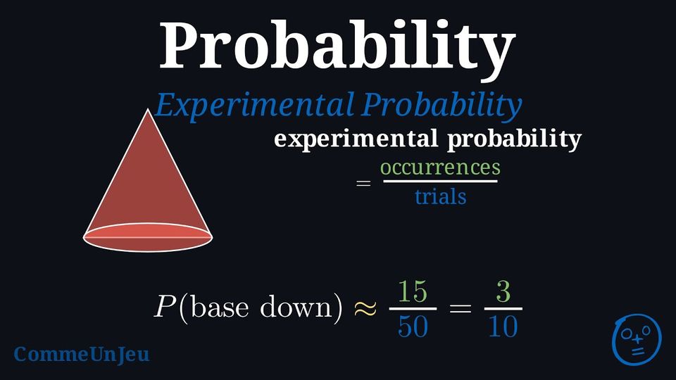
Proposition — Fluctuation and Stabilisation
An experiment is repeated \(n\) times under the same conditions, each repetition having no influence on the others, and the frequency of an event of probability \(p\) is observed. - Fluctuation: for a fixed \(n\), the frequency can change from one series to another. Two series of the same length do not necessarily give the same frequency.
- Stabilisation: when \(n\) grows, the frequencies tend to move closer to \(p\). Long series usually stray less from \(p\) than short ones.
- Expected count: over \(n\) repetitions, the expected count of the event is \(n \times p\); the observed count is about \(n \times p\), in the sense that the observed frequency, the count divided by \(n\), is usually close to \(p\). “About”: the observed count is not known in advance, and it need not equal \(n \times p\) exactly.
Example
Two pupils each throw a fair die again and again, and record the frequency of “getting a \(6\)” as the number \(n\) of throws grows (the \(n\)-axis is not drawn to scale). 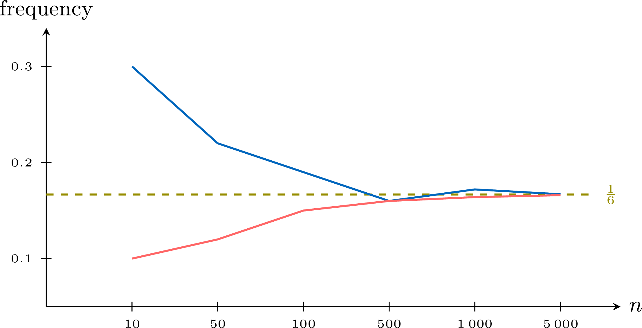
- For which values of \(n\) do the two frequencies differ the most? What is this phenomenon called?
- Around which value do the two curves settle? Why?
- How many sixes are expected over \(1\,200\) throws?
- After \(600\) throws, one pupil has only \(85\) sixes instead of the \(100\) expected. Will the following throws “make up” for it?
- For the small values of \(n\): at \(n = 10\) the frequencies are \(0.30\) and \(0.10\). This is the fluctuation: short series differ a lot from one another.
- Both curves settle around \(\dfrac{1}{6} \approx 0.167\), the probability of getting a \(6\) with a fair die. This is the stabilisation: the longer the series, the closer its frequency is to the probability.
- \(1\,200 \times \dfrac{1}{6} = \textcolor{colordef}{200}\): about \(200\) sixes are expected — a real series will give a number close to \(200\), without \(200\) itself being guaranteed.
- No. The die has no memory: each throw still has a probability \(\dfrac{1}{6}\) of giving a \(6\). The frequency comes close to \(\dfrac{1}{6}\) because the \(15\) missing sixes weigh less and less among more and more throws — they are diluted, not made up for.
Skills to practice
- Calculating an Expected Count
V
Going further
Skills to practice
- Solving Multi-Step Probability Problems
- Investigating Patterns in Tables of Outcomes
- Quiz
Jump to section