International Baccalaureate · MYP 2
Probability
I
Sample Spaces and Events
I.1
The Sample Space
Example
What are all the possible outcomes when you flip a coin? 
The outcomes are Heads (H) =  and Tails (T) =
 .
and Tails (T) = . Example
What are the outcomes when you roll a six-sided die?
The outcomes are \(1 = \) , \(2 = \)
 , \(3 = \)
 , \(4 = \)
 , \(5 = \)
 and \(6 = \)
 .
, \(2 = \), \(3 = \), \(4 = \), \(5 = \) and \(6 = \). Definition — Sample Space
The sample space, denoted \(U\), is the set of all possible outcomes of a random experiment. A single outcome is denoted \(x\). If the experiment has \(n\) outcomes, we write $$U = \{x_1, x_2, \dots, x_n\}.$$ Example
What’s the sample space when you flip a coin?
The sample space is \(U = \{\text{Heads}, \text{Tails}\} = \{\),\(\}\), or just \(U = \{\text{H}, \text{T}\}\) for short. It has two outcomes: \(x_1 = \text{H}\) and \(x_2 = \text{T}\).
,\(\}\), or just \(U = \{\text{H}, \text{T}\}\) for short. It has two outcomes: \(x_1 = \text{H}\) and \(x_2 = \text{T}\). Example
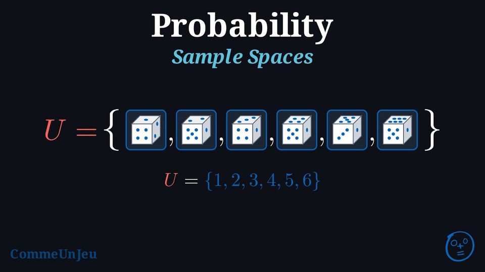
What’s the sample space when you roll a six-sided die?
The sample space is \(U = \{1, 2, 3, 4, 5, 6\} = \{\),,,,,\(\}\).
,,,,,\(\}\). 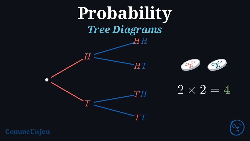
A multi-step experiment is a random experiment made up of a sequence of two or more simple steps. For example, flipping two coins is a multi-step experiment composed of two actions: flipping the first coin and then flipping the second.
In many multi-step experiments, we can find the total number of possible outcomes by multiplying the number of outcomes at each step. To display all the combined outcomes, we can use tools like lists, tables, or tree diagrams.
In many multi-step experiments, we can find the total number of possible outcomes by multiplying the number of outcomes at each step. To display all the combined outcomes, we can use tools like lists, tables, or tree diagrams.
Method — Representing Sample Spaces for Multi-Step Experiments
When an experiment has more than one step, the sample space can be represented in several ways: - by listing all possible ordered outcomes;
- using a table (best for two-step experiments);
- using a tree diagram (useful for any number of steps).
Example
For the experiment of tossing two coins, represent the sample space by: - listing all possible outcomes;
- using a table;
- using a tree diagram.
- List:
Each outcome records the result of coin 1 first, then coin 2: $$\{\textcolor{colordef}{H}\textcolor{colorprop}{H}, \textcolor{colordef}{H}\textcolor{colorprop}{T}, \textcolor{colordef}{T}\textcolor{colorprop}{H}, \textcolor{colordef}{T}\textcolor{colorprop}{T}\}$$ - Table:
\(\begin{aligned} & \textcolor{colorprop}{\text{coin 2}} \\ \textcolor{colordef}{\text{coin 1}} \end{aligned} \) \(\textcolor{colorprop}{H}\) \(\textcolor{colorprop}{T}\) \(\textcolor{colordef}{H}\) \(\textcolor{colordef}{H}\textcolor{colorprop}{H}\) \(\textcolor{colordef}{H}\textcolor{colorprop}{T}\) \(\textcolor{colordef}{T}\) \(\textcolor{colordef}{T}\textcolor{colorprop}{H}\) \(\textcolor{colordef}{T}\textcolor{colorprop}{T}\) - Tree diagram:
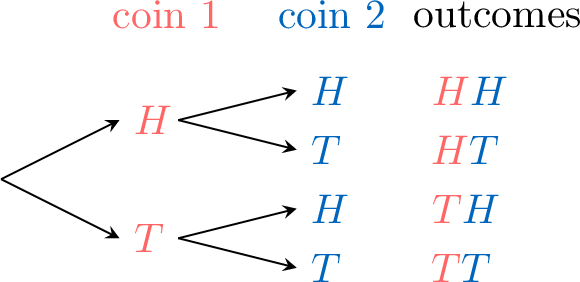
Skills to practice
- Finding the Sample Space
- Writing the Sample Space
I.2
Events
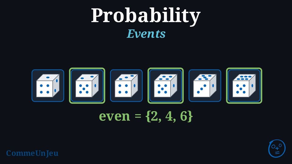
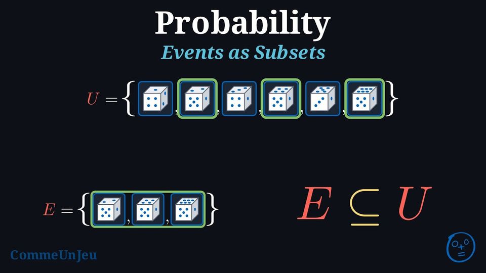
Once we know all the possible outcomes of an experiment (the sample space), we can focus on specific outcomes we are interested in. An event is a set of outcomes (it may contain one outcome, several outcomes, or even none at all).
Definition — Event
An event (often denoted by a capital letter like \(E\)) is a subset of the sample space. Example
For the experiment of rolling a die, list the outcomes in the event \(E\): “rolling an even number”.
Among the outcomes of the sample space \(U = \{1, 2, 3, 4, 5, 6\} = \{\),,,,,\(\}\), the event of rolling an even number is \(E = \{2, 4, 6\} = \{\),,\(\}\).
,,,,,\(\}\), the event of rolling an even number is \(E = \{2, 4, 6\} = \{\),,\(\}\). Skills to practice
- Finding the Outcomes of an Event
I.3
Singleton Events
Definition — Singleton Event
For an outcome \(x\), the event \(\{x\}\) that contains only \(x\) is called a singleton (a set with a single element, written with braces). For example, on a die the singleton \(\{3\} = \{\)\(\}\) is the event “rolling a 3”. Skills to practice
- Listing the Outcomes and the Events
I.4
Complementary Events
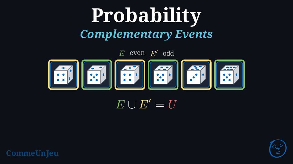
In probability, it is often useful to consider the outcomes that do not belong to a specific event. This set of “other” outcomes is known as the complementary event. It represents everything in the sample space that is outside the original event. The complement of an event \(E\) is denoted by \(E'\).
Definition — Complementary Event
The complementary event of an event \(E\), denoted \(E'\) or \(\overline{E}\), is the set of all outcomes in the sample space that are not in \(E\). Example
In the experiment of rolling a fair six-sided die, let \(E\) be the event “rolling an even number”. Find the complementary event, \(E'\).
The sample space is \(U = \{1, 2, 3, 4, 5, 6\} = \{\),,,,,\(\}\).
The event is \(E = \{2, 4, 6\} = \{\),,\(\}\).
The complementary event \(E'\) contains all outcomes in the sample space that are not in \(E\).
Therefore, \(E' = \{1, 3, 5\} = \{\),,\(\}\). This is the event “rolling an odd number”.
,,,,,\(\}\).The event is \(E = \{2, 4, 6\} = \{\)
,,\(\}\).The complementary event \(E'\) contains all outcomes in the sample space that are not in \(E\).
Therefore, \(E' = \{1, 3, 5\} = \{\)
,,\(\}\). This is the event “rolling an odd number”. Skills to practice
- Finding the Complementary Event
II
Describing Probability
II.1
Probability Words
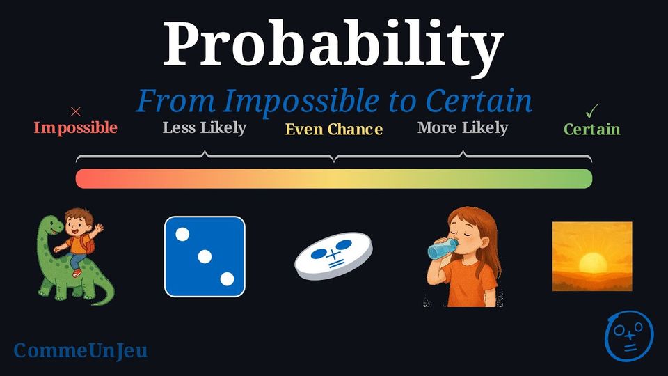
We use special words to describe the chance of an event happening. We can place these words on a line from least likely to most likely.
Definition — Probability Line

- Impossible: It can’t happen.
Example: Riding a dinosaur. - Less likely: It probably won’t happen.
Example: Rolling a die and getting a 3. - Even chance: It has the same chance to happen or not to happen.
Example: Tossing a coin and getting heads. - More likely: It will probably happen.
Example: Drinking water at school today. - Certain: It will happen.
Example: The sun will rise tomorrow.
Riding a dinosaur, drinking water at school and the sunrise are everyday happenings, not events of an experiment whose outcomes are listed. In an experiment, an event is impossible when no outcome makes it happen, and certain when every outcome makes it happen: with a die, “getting a 7” is impossible and “getting a number from 1 to 6” is certain.
Skills to practice
- Classifying Events on the Probability Scale
II.2
Probability as a Number from 0 to 1
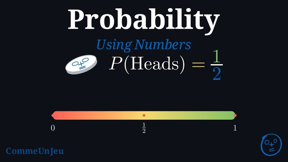
When you flip a fair coin, there are two possible outcomes: heads or tails. The chance of getting heads is 1 out of 2. We can write this as a fraction: 
Definition — Probability
The probability of an event \(E\), written \(P(E)\), is a number that tells us how likely the event is to happen. It is always between \(0\) (impossible) and \(1\) (certain). In other words, for any event \(E\), we have \(0 \leq P(E) \leq 1\). 
Skills to practice
- Making Decisions Using Probabilities
III
Calculating Probabilities
III.1
The Probability of an Event
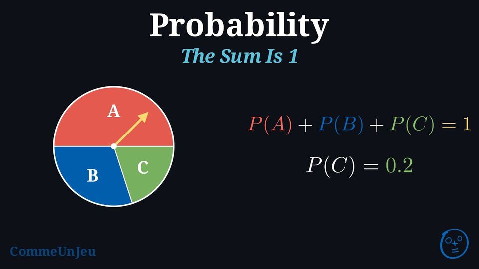
Proposition — Sum of the Probabilities
In a random experiment, the probabilities of all the outcomes add up to \(1\): $$\textcolor{colorprop}{P(\text{outcome}_1) + P(\text{outcome}_2) + \dots + P(\text{outcome}_n) = 1}$$ 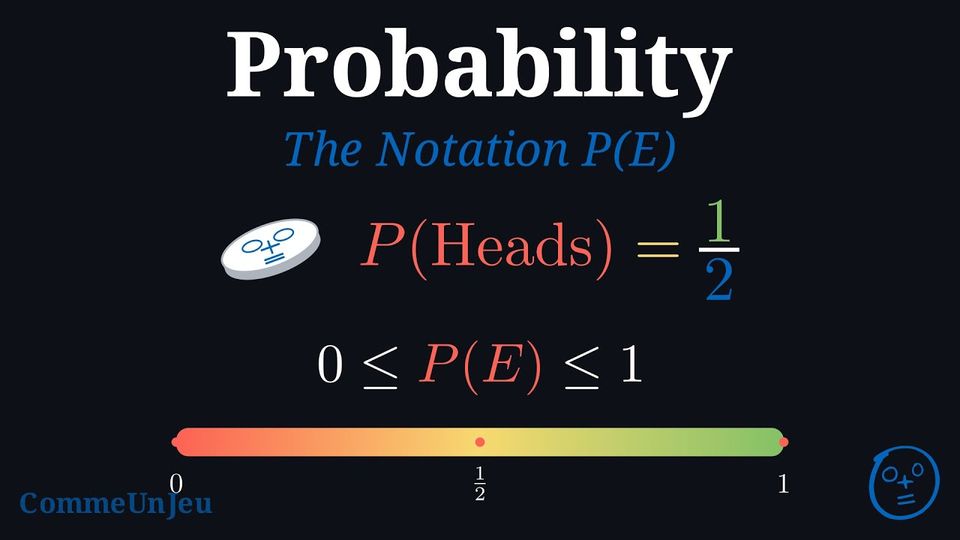
Probability of an Outcome
An outcome \(x\) and its singleton event \(\{x\}\) — the set with a single element — describe the same result: speaking of the chance of an outcome is therefore speaking of the chance of an event. The probability of the outcome is the probability of that event, written \(P(\{x\})\). In practice, we allow ourselves to write \(P(x)\) for \(P(\{x\})\) — for instance \(P(3)\) for the probability of rolling a 3.
Proposition — Probability of an Event
The probability of an event is the sum of the probabilities of its outcomes: $$\textcolor{colorprop}{P(\text{event}) = \text{sum of the probabilities of its outcomes}}$$
With this notation, the two rules above read: the probabilities of the outcomes \(x_1, \dots, x_n\) of \(U\) add up to \(1\), and the probability of an event \(E\) is the sum of the probabilities of the outcomes that make up \(E\). In particular, the certain event is \(U\) itself, with \(P(U) = 1\), and the impossible event is the empty set \(\emptyset\): it contains no outcome, and \(P(\emptyset) = 0\).
Skills to practice
- Calculating the Probability of an Event
III.2
Equally Likely Outcomes
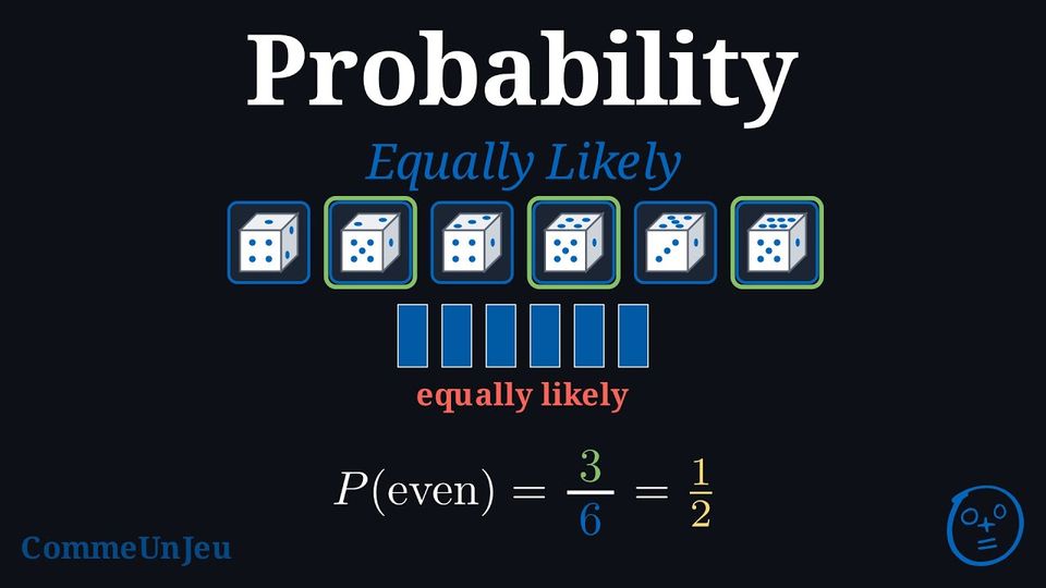
Have you ever flipped a fair coin or rolled a fair die? Their symmetry makes it reasonable to assume that each outcome has the same chance as the others: this is a hypothesis of the model, not something we can prove. We call these equally likely outcomes.
Definition — Equally Likely
When all the outcomes in the sample space are equally likely to occur, the probability of an event \(E\) is: $$P(E) = \frac{\text{number of outcomes in the event}}{\text{number of outcomes in the sample space}}$$ Example
What’s the probability of rolling an even number with a fair six-sided die? - Sample space \(U = \{1, 2, 3, 4, 5, 6\}\) (6 outcomes).
- \(E = \{2, 4, 6\}\) (3 outcomes).
- $$\begin{aligned} P(E) &= \frac{3}{6} \\ &= \frac{1}{2} \end{aligned}$$
Skills to practice
- Finding Probabilities with Dice and Spinners
- Calculating and Comparing Probabilities
- Calculating the Probability of a Singleton
III.3
The Complement Rule
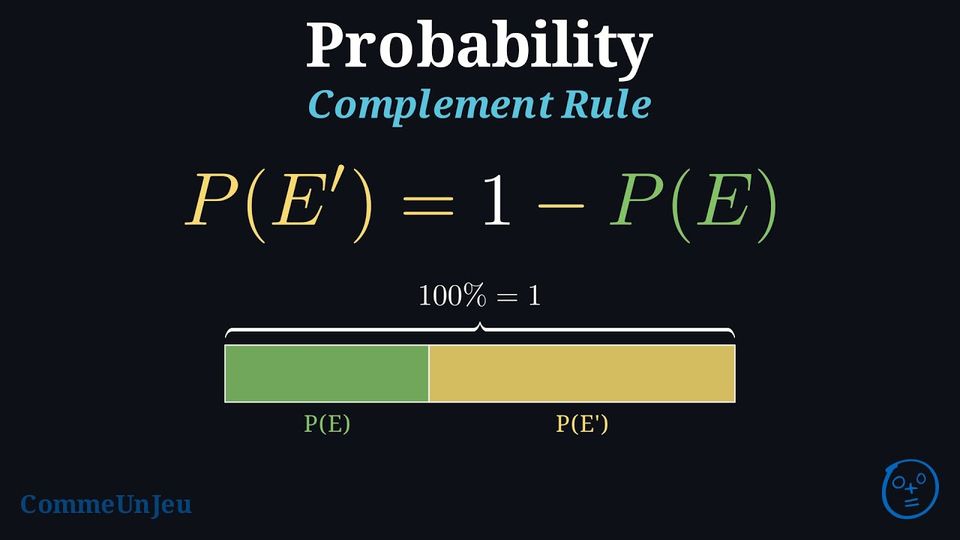
Tomorrow's weather is modelled by an experiment with two outcomes: \(U = \{\text{rain}, \text{no rain}\}\). If there is a \(40\pourcent\) chance of rain tomorrow, what is the chance that it will not rain? \(100\pourcent - 40\pourcent = 60\pourcent\) This calculation is an application of the complement rule, since the event \(\{\text{no rain}\}\) is the complementary event of \(\{\text{rain}\}\). It is a shortcut to find the probability that an event does not happen.
Proposition — Complement Rule
For any event \(E\) and its complementary event \(E'\), their probabilities must add up to \(1\) (or \(100\pourcent\)): $$\textcolor{colorprop}{P(E) + P(E') = 1}$$ This leads to the useful formula for finding the probability of the complement: $$\textcolor{colorprop}{P(E') = 1 - P(E)}$$
The complementary event \(E'\) is made of exactly the outcomes of \(U\) that are not in \(E\). So every outcome of \(U\) lies in exactly one of \(E\) and \(E'\): together they split \(U\) into two parts that overlap nowhere. 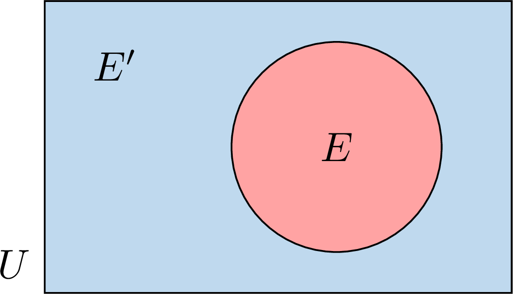
The probability of an event is the sum of the probabilities of its outcomes. Adding \(P(E)\) and \(P(E')\) therefore counts the probability of every outcome of \(U\) exactly once: $$\begin{aligned}[t] P(E) + P(E') &= \text{(sum of the probabilities of all the outcomes of } U\text{)} && \text{(every outcome is in \(E\) or in \(E'\))}\\
&= P(U) && \text{(the whole sample space)}\\
&= 1. \end{aligned}$$ Subtracting \(P(E)\) from both sides gives \(P(E') = 1 - P(E)\).
Example
Farid's homework tonight is modelled by an experiment with two outcomes: \(U = \{\text{on time}, \text{late}\}\). Farid has a \(0.8\) (\(80\pourcent\)) chance of finishing his homework on time tonight: the event \(E = \{\text{on time}\}\) has probability \(0.8\). What is the probability that he does not finish on time?
The complementary event is \(E' = \{\text{late}\}\), the event “Farid does not finish his homework on time”. Using the complement rule: $$\begin{aligned} P(E') &= 1 - P(E) \\
&= 1 - 0.8 \\
&= 0.2 \end{aligned}$$ There is a \(0.2\) (or \(20\pourcent\)) probability that he does not finish on time.
Skills to practice
- Applying the Complement Rule
- Investigating Patterns in Multi-Step Experiments
IV
Experimental Probability
IV.1
Experimental Probability
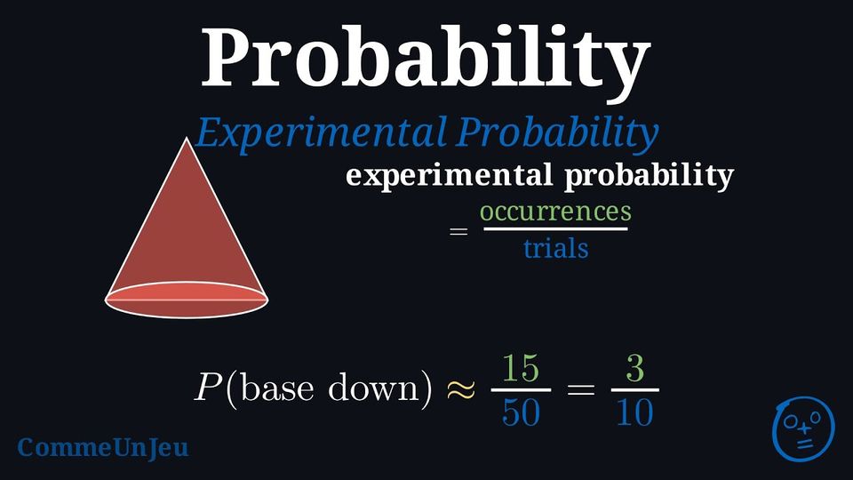
So far, we have calculated theoretical probability: a number computed from equally likely outcomes, before any experiment. For example, a fair coin has two equally likely outcomes, heads and tails, so we say \(P(\text{Heads}) = \frac{1}{2}\).
But what if the outcomes are not equally likely? Then counting them does not give the probability. In these cases, we can do an experiment to estimate the probability.
But what if the outcomes are not equally likely? Then counting them does not give the probability. In these cases, we can do an experiment to estimate the probability.
Isaac wants to find the probability that a cone he drops will land on its base. The possible outcomes are “base down” or “on its side”. 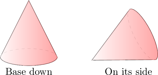
Because of the cone’s shape, nothing says that these two outcomes are equally likely: no symmetry allows us to give them equal probabilities, so a direct calculation is impossible. Isaac therefore estimates the probability by experiment. He tosses the cone 50 times (50 trials) and records the results:
- Base down: 15 times.
- On its side: 35 times.
Definition — Relative Frequency
The relative frequency of an event in a series of trials is the quotient $$ \text{Frequency} = \frac{\text{Number of times the event occurs}}{\text{Total number of trials}} $$ It is a number between \(0\) and \(1\) which describes the series actually observed. When the experiment is repeated many times, this frequency gives an estimate of the probability of the event, also called its experimental probability. In general, the larger the number of trials, the more reliable this estimate is. 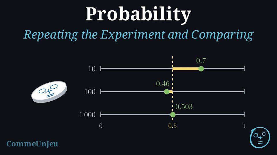
Léa rolls a fair die. She knows that \(P(6) = \frac{1}{6}\). She rolls it \(12\) times and never gets a \(6\). Sami says: “your die is loaded”. Léa answers: “one chance in six, so in \(12\) rolls I should have had exactly two sixes”. Who is correct?
Neither of them. The probability \(\frac{1}{6}\) does not promise two sixes in \(12\) rolls: it says that, if the die is rolled a very large number of times, about one roll in six gives a \(6\). Twelve rolls is very few: getting no \(6\) at all happens quite often with a perfectly fair die. So Sami cannot conclude that the die is loaded, and Léa was wrong to expect exactly two. To compare what happens with what was calculated, the experiment must be repeated many more times.
Definition — Part of the Trials
When an experiment is repeated, each repetition is a trial. The part of the trials that gave a result is the number of trials that gave it, divided by the total number of trials: $$\text{part of the trials} = \frac{\text{number of trials that gave the result}}{\text{total number of trials}}.$$ Like a probability, it is a number between \(0\) and \(1\), and it can be written as a fraction, a decimal or a percentage. If \(46\) tosses out of \(100\) gave heads, the part of the trials that gave heads is \(\frac{46}{100} = 0.46 = 46\pourcent\). Method — Comparing a Series of Trials to the Calculated Probability
- Calculate the probability of the result, in a situation where all outcomes are equally likely: a fair coin, a fair die, a well-balanced wheel.
- Repeat the experiment many times, without changing anything between two trials: the same die, thrown the same way. Each trial is a new experiment, with the same chances as the first one — the die has no memory.
- Count and divide: for the result studied, write the part of the trials that gave it.
- Compare the part of the trials with the calculated probability, written in the same form.
- Read the gap. With few trials, the gap is often large. With many trials, the part of the trials is most often close to the calculated probability — it never has to hit it exactly, and it can move away again from one trial to the next. A gap, on its own, does not prove that the die is loaded.
Example
A fair coin is tossed. After \(10\) tosses, \(7\) gave heads; after \(100\) tosses, \(46\) gave heads; after \(1\,000\) tosses, \(503\) gave heads. Compare, each time, the part of the trials that gave heads with the calculated probability.
The coin is fair: \(P(\text{heads}) = \frac{1}{2} = 0.5\). The parts of the trials are:
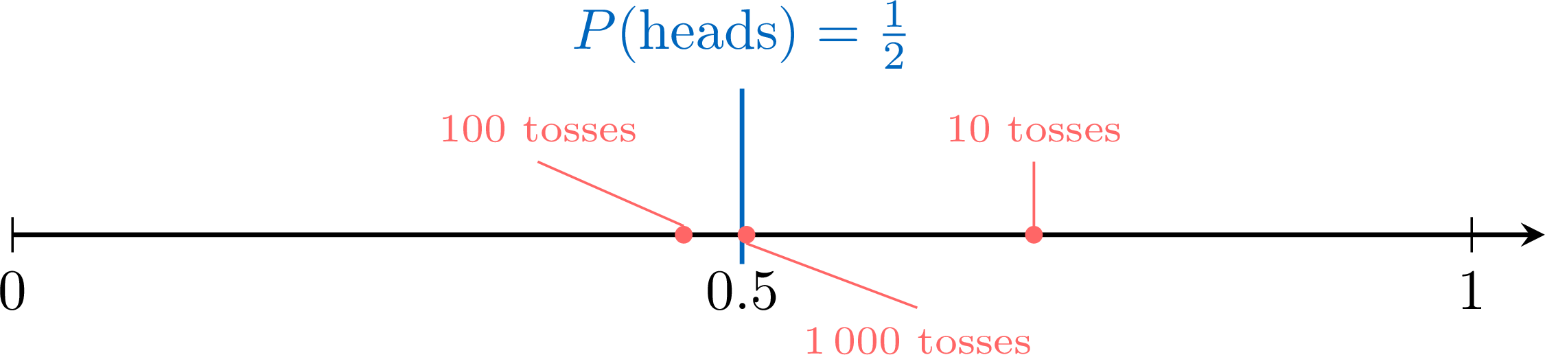
After \(10\) tosses the part is \(0.7\), far from \(0.5\) — with so few tosses, that is not surprising. After \(100\) it is \(0.46\), closer. After \(1\,000\) it is \(0.503\), very close. The more the experiment is repeated, the closer the part of the trials tends to come to the calculated probability, without ever having to equal it: \(503\) is not \(500\).
| Tosses | Heads | Part of the trials | Gap with \(0.5\) |
| \(10\) | \(7\) | \(\frac{7}{10} = 0.7\) | \(0.2\) |
| \(100\) | \(46\) | \(\frac{46}{100} = 0.46\) | \(0.04\) |
| \(1\,000\) | \(503\) | \(\frac{503}{1000} = 0.503\) | \(0.003\) |
What a Gap Means
A gap between the part of the trials and the calculated probability is not a mistake, and it is not a proof either. With \(12\) rolls, a fair die can easily give no \(6\) at all, or three of them. What counts is the tendency over many trials: on a large number of rolls, the part of sixes settles near \(\frac{1}{6}\). And the other way round: if, after a thousand rolls, the part of sixes stayed far from \(\frac{1}{6}\), one would have good reasons to doubt that the die is fair — but no one can decide that on twelve rolls.
Proposition — Fluctuation of Frequencies
For a fixed number of trials \(n\), the observed frequencies generally vary from one series to another: they fluctuate.When \(n\) becomes large, the frequency of each outcome tends to get closer to its probability. This is an experimental observation.
Skills to practice
- Calculating Experimental Probabilities in Percentage Form
- Reading Frequencies and Comparing Them with the Probability
- Watching the Frequency Approach the Probability
- Comparing Trials with the Calculated Probability
- Interpreting Fluctuation
V
Going further
Skills to practice
- Reasoning with Events and Probability
- Solving Probability Problems
- Quiz
Jump to section