International Baccalaureate · PYP 5
Probability
I
Outcomes, Events and Two-Step Experiments
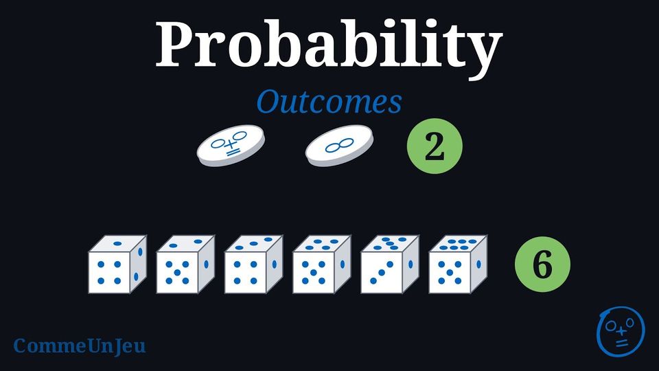
Some actions have a result we cannot predict — flipping a coin, rolling a die, or playing a game. We call such an action a random experiment: it can be repeated under the same conditions, all its possible results are known in advance, but nobody can tell with certainty which one will happen. Probability is a mathematical way to measure how likely an event of the experiment is, such as “rolling a 6” when a die is rolled.
Definition — Outcome
An outcome is one possible result of a random experiment. Definition — All Possible Outcomes
All possible outcomes are the complete list of all the outcomes that can happen in a random experiment. Example
What are all the possible outcomes when you flip a coin? 
All possible outcomes are Heads (H)= and Tails (T)=
 .
and Tails (T)=. Example
What are all the possible outcomes when you roll a six-sided die?
All possible outcomes are 1= , 2=
 , 3=
 , 4=
 , 5=
 , and 6=
 .
, 2=, 3=, 4=, 5=, and 6=. 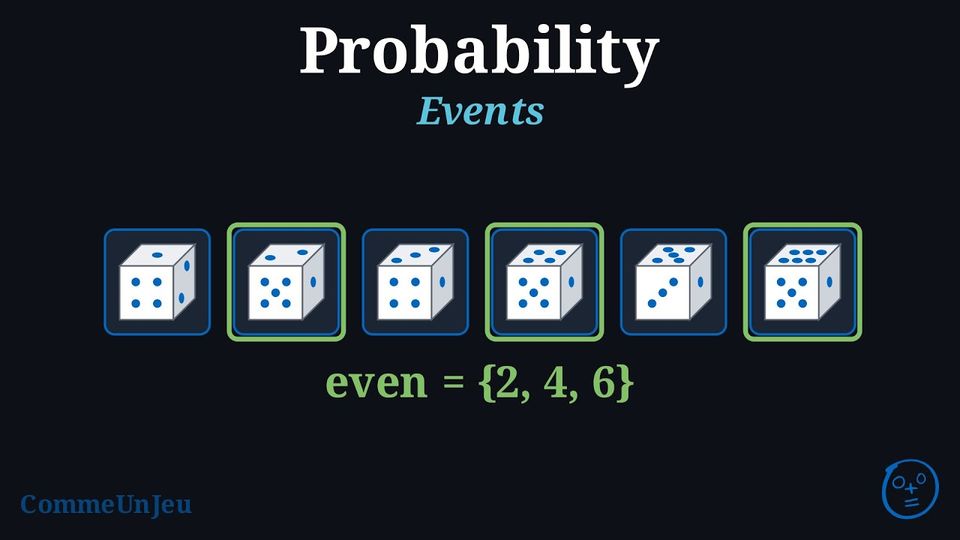
Once we know all the possible outcomes of an experiment (the sample space), we can focus on specific results we are interested in. These specific results are called events: an event can contain several outcomes, a single outcome, or even none (the impossible event).
Definition — Event
An event is a set of outcomes from the set of all possible outcomes. Example
In the experiment of rolling a die, find the outcomes that correspond to rolling an even number.
The outcomes for “rolling an even number” are 2=, 4=, and 6=.
, 4=, and 6=. 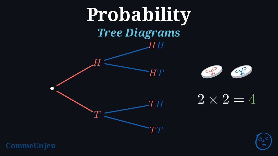
Léa rolls a four-sided die, then rolls it again, and writes the two results one after the other: \(3\), then \(1\). Sami counts out loud: “four results at the first roll, four at the second, that makes eight in all”. Léa is not convinced; she starts writing them down, \(11\), \(12\), \(13\), and soon loses track. The outcomes of a two-step experiment cannot be counted in one's head: it takes a tool that lists them all without forgetting any.
Definition — Outcome of a two-step experiment
Some random experiments are made of two steps: toss a coin then toss it again, roll two dice one after the other, spin a wheel twice, draw a ball, put it back and draw again. The two results are looked at together: an outcome of such an experiment is the pair made of a result of the first step followed by a result of the second. We write the two results side by side: \(\textcolor{colordef}{\text{H}}\textcolor{colorprop}{\text{T}}\) means heads at the first toss, then tails at the second. To find all the outcomes without forgetting any, we use a table or a tree. Method — The table of outcomes
- One row per outcome of the first step, one column per outcome of the second.
- Each cell is one outcome of the two-step experiment: write in it the result of its row followed by the result of its column.
- Count: the number of outcomes is the number of cells, that is the number of rows times the number of columns. This works because the second step has the same outcomes whatever the first one gave — the same die is rolled again, the ball is put back in the bag.
Method — The tree of outcomes
- One branch per outcome of the first step, drawn from the trunk.
- At the end of each of these branches, one branch per outcome of the second step — the same ones each time.
- Each complete path, from the trunk to the end, is one outcome: read it from left to right.
- Count: the number of outcomes is the number of paths, that is the number of ends on the right.
Example
A fair coin is tossed twice. Find all the outcomes of this experiment, with a table and with a tree.
The first step has two outcomes, heads (H) and tails (T); so does the second.
The table has \(2\) rows and \(2\) columns, so \(2 \times 2 = 4\) cells: the outcomes are HH, HT, TH and TT. The tree gives the same four, read along its four paths. 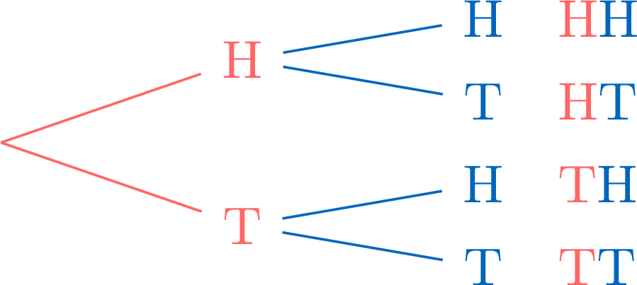
| \(\begin{aligned} & \textcolor{colorprop}{\text{2nd toss}} \\ \textcolor{colordef}{\text{1st toss}} \end{aligned}\) | \(\textcolor{colorprop}{\text{H}}\) | \(\textcolor{colorprop}{\text{T}}\) |
| \(\textcolor{colordef}{\text{H}}\) | \(\textcolor{colordef}{\text{H}}\textcolor{colorprop}{\text{H}}\) | \(\textcolor{colordef}{\text{H}}\textcolor{colorprop}{\text{T}}\) |
| \(\textcolor{colordef}{\text{T}}\) | \(\textcolor{colordef}{\text{T}}\textcolor{colorprop}{\text{H}}\) | \(\textcolor{colordef}{\text{T}}\textcolor{colorprop}{\text{T}}\) |
Example
Maya rolls a fair four-sided die, then rolls it again. How many outcomes does this experiment have? How many of them realise the event “an even number at both rolls”?
The die has \(4\) outcomes at each roll: the table has \(4\) rows and \(4\) columns, so \(4 \times 4 = 16\) outcomes.
The outcomes in bold are those of the event: an even number at the first roll, and an even number at the second. There are \(4\) of them out of \(16\).
| \(\begin{aligned} & \textcolor{colorprop}{\text{2nd roll}} \\ \textcolor{colordef}{\text{1st roll}} \end{aligned}\) | \(\textcolor{colorprop}{\text{1}}\) | \(\textcolor{colorprop}{\text{2}}\) | \(\textcolor{colorprop}{\text{3}}\) | \(\textcolor{colorprop}{\text{4}}\) |
| \(\textcolor{colordef}{\text{1}}\) | \(\textcolor{colordef}{\text{1}}\textcolor{colorprop}{\text{1}}\) | \(\textcolor{colordef}{\text{1}}\textcolor{colorprop}{\text{2}}\) | \(\textcolor{colordef}{\text{1}}\textcolor{colorprop}{\text{3}}\) | \(\textcolor{colordef}{\text{1}}\textcolor{colorprop}{\text{4}}\) |
| \(\textcolor{colordef}{\text{2}}\) | \(\textcolor{colordef}{\text{2}}\textcolor{colorprop}{\text{1}}\) | \(\textcolor{colordef}{\text{2}}\textcolor{colorprop}{\text{2}}\) | \(\textcolor{colordef}{\text{2}}\textcolor{colorprop}{\text{3}}\) | \(\textcolor{colordef}{\text{2}}\textcolor{colorprop}{\text{4}}\) |
| \(\textcolor{colordef}{\text{3}}\) | \(\textcolor{colordef}{\text{3}}\textcolor{colorprop}{\text{1}}\) | \(\textcolor{colordef}{\text{3}}\textcolor{colorprop}{\text{2}}\) | \(\textcolor{colordef}{\text{3}}\textcolor{colorprop}{\text{3}}\) | \(\textcolor{colordef}{\text{3}}\textcolor{colorprop}{\text{4}}\) |
| \(\textcolor{colordef}{\text{4}}\) | \(\textcolor{colordef}{\text{4}}\textcolor{colorprop}{\text{1}}\) | \(\textcolor{colordef}{\text{4}}\textcolor{colorprop}{\text{2}}\) | \(\textcolor{colordef}{\text{4}}\textcolor{colorprop}{\text{3}}\) | \(\textcolor{colordef}{\text{4}}\textcolor{colorprop}{\text{4}}\) |
Table or tree? Both list exactly the same outcomes. The table is compact and shows at a glance that the number of outcomes is a product; the tree shows the order of the two steps, and it keeps working for three steps or more, where a table no longer would.
Skills to practice
- Completing the Table of Outcomes
- Reading the Tree of Outcomes
II
Representing Probabilities as Numbers
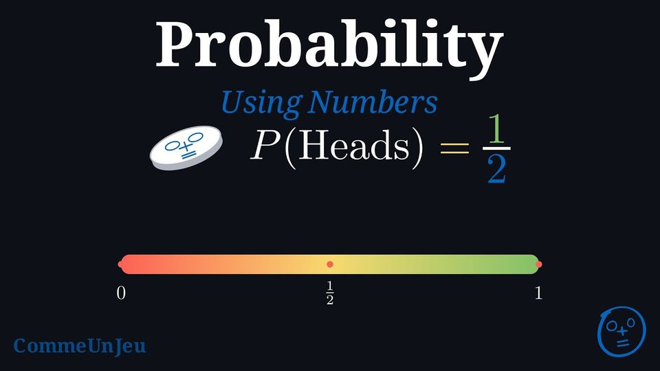
When you flip a fair coin, there are two possible outcomes: heads or tails. The chance of getting heads is 1 out of 2. We can write this as a fraction: 
Definition — Probability
The probability of an event, written \(P(\text{event})\), is a number from 0 (impossible) to 1 (certain). 
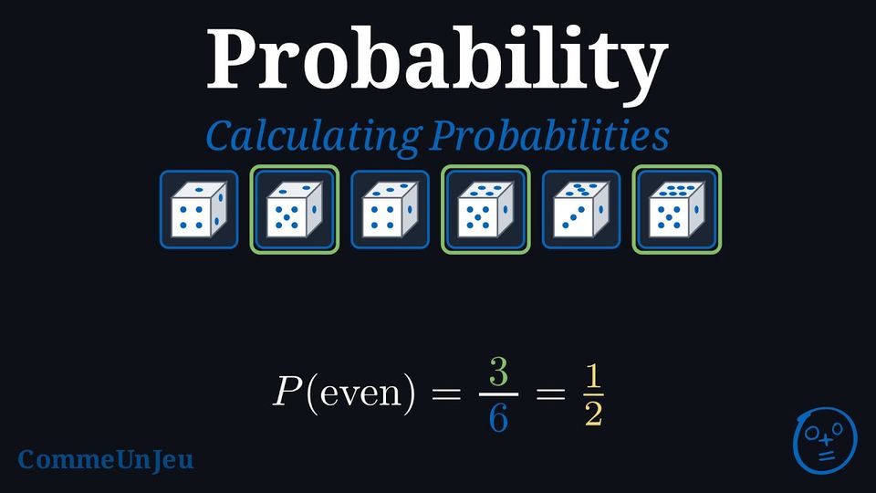
In many experiments, each outcome has the same chance of happening. For example, a fair coin is just as likely to land on heads as it is on tails. When we roll a fair die, each number from 1 to 6 has the same chance of appearing. We call these equally likely outcomes.
Definition — Calculating Probability with Equally Likely Outcomes
When all outcomes of an experiment are equally likely, we can calculate the probability of an event using a simple formula: $$P(\text{event}) = \frac{\text{Number of favourable outcomes}}{\text{Total number of possible outcomes}}$$ “Favourable outcomes” are the outcomes that match the event we are interested in. Example
A fair six-sided die is rolled. Calculate the probability of rolling an even number. - Total number of possible outcomes: A die has 6 faces, so there are 6 possible outcomes: \(1\), \(2\), \(3\), \(4\), \(5\) and \(6\).
- Number of favourable outcomes: The event is “rolling an even number”. The outcomes that are even are \(2\), \(4\) and \(6\). There are 3 favourable outcomes.
- Calculate the probability: $$\begin{aligned} P(\text{rolling an even number}) &= \frac{\text{Number of favourable outcomes}}{\text{Total number of possible outcomes}} \\ &= \frac{3}{6} \\ &= \frac{1}{2} \end{aligned}$$
Method — Expressing Probabilities in Different Forms
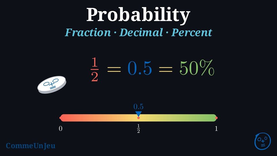
We can write probabilities in three different ways: as fractions, decimals, or percentages. These three forms represent the same probability, but look different. Example
A fair spinner has 4 equal parts, 1 of them red: \(P(\text{red}) = \frac{1}{4}\). Represent this probability as a decimal and a percentage.
The parts are numbered from \(1\) to \(4\): they are the \(4\) equally likely outcomes, and “red” is part \(1\) alone, so \(P(\text{red}) = \frac{1}{4}\). 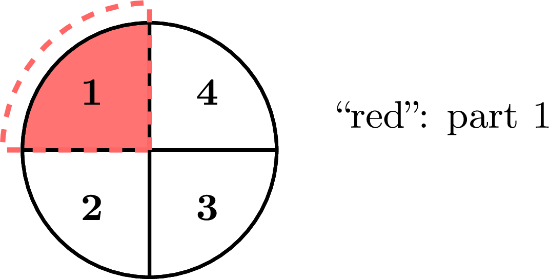
- Fraction: \( \frac{1}{4} \)
- Decimal: To convert a fraction to a decimal, divide the numerator by the denominator: $$ 1 \div 4 = 0.25 $$
- Percentage: To convert a decimal to a percentage, multiply by 100 and add the percent sign: $$ 0.25 = 0.25 \times 100\pourcent = 25\pourcent $$
Skills to practice
- Calculating Probabilities in Decimal Form
- Calculating Probabilities in Percentage Form
- Placing and Comparing Probabilities
III
Calculating a Probability in Two Steps
Method — Calculating a Probability in a Two-Step Experiment
Nothing new: the same rule applies word for word, with the cells of the table, or the ends of the tree, as the outcomes. - Check that the outcomes are equally likely: each step is fair (a coin, a die, a wheel with equal sectors), and the second step is carried out under the same conditions as the first (the same die is rolled again, the ball is put back in the bag). We then assume that all the cells have the same chance.
- Count the cells, or the ends, that realise the event.
- Divide that number by the total number of cells, or of ends.
| \(\begin{aligned} & \textcolor{colorprop}{\text{2nd roll}} \\ \textcolor{colordef}{\text{1st roll}} \end{aligned}\) | \(\textcolor{colorprop}{\text{1}}\) | \(\textcolor{colorprop}{\text{2}}\) | \(\textcolor{colorprop}{\text{3}}\) | \(\textcolor{colorprop}{\text{4}}\) |
| \(\textcolor{colordef}{\text{1}}\) | \(\textcolor{colordef}{\text{1}}\textcolor{colorprop}{\text{1}}\) | \(\textcolor{colordef}{\text{1}}\textcolor{colorprop}{\text{2}}\) | \(\textcolor{colordef}{\text{1}}\textcolor{colorprop}{\text{3}}\) | \(\textcolor{colordef}{\text{1}}\textcolor{colorprop}{\text{4}}\) |
| \(\textcolor{colordef}{\text{2}}\) | \(\textcolor{colordef}{\text{2}}\textcolor{colorprop}{\text{1}}\) | \(\textcolor{colordef}{\text{2}}\textcolor{colorprop}{\text{2}}\) | \(\textcolor{colordef}{\text{2}}\textcolor{colorprop}{\text{3}}\) | \(\textcolor{colordef}{\text{2}}\textcolor{colorprop}{\text{4}}\) |
| \(\textcolor{colordef}{\text{3}}\) | \(\textcolor{colordef}{\text{3}}\textcolor{colorprop}{\text{1}}\) | \(\textcolor{colordef}{\text{3}}\textcolor{colorprop}{\text{2}}\) | \(\textcolor{colordef}{\text{3}}\textcolor{colorprop}{\text{3}}\) | \(\textcolor{colordef}{\text{3}}\textcolor{colorprop}{\text{4}}\) |
| \(\textcolor{colordef}{\text{4}}\) | \(\textcolor{colordef}{\text{4}}\textcolor{colorprop}{\text{1}}\) | \(\textcolor{colordef}{\text{4}}\textcolor{colorprop}{\text{2}}\) | \(\textcolor{colordef}{\text{4}}\textcolor{colorprop}{\text{3}}\) | \(\textcolor{colordef}{\text{4}}\textcolor{colorprop}{\text{4}}\) |
Skills to practice
- Calculating a Probability in a Two-Step Experiment
IV
Experimental Probability
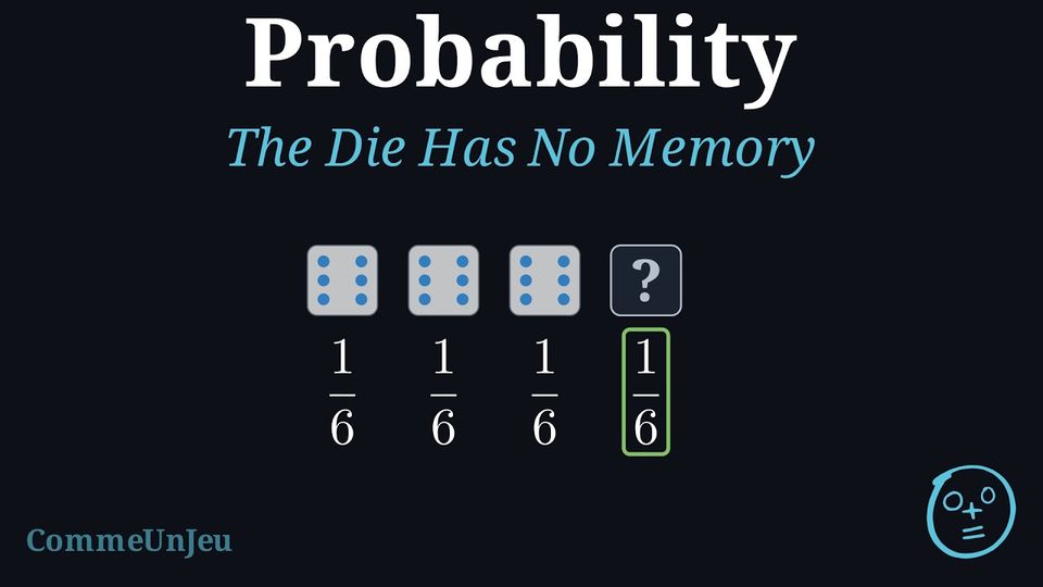
Lina rolls a fair die three times and gets a \(6\) each time. 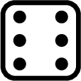
“The next one will certainly not be a \(6\),” she says, “a \(6\) has already come out three times.” Sami disagrees: “On the contrary, the die is lucky today: it will give a \(6\) again.” Which of them is correct?
Repeating the same experiment. When a fair die is rolled again under the same conditions, knowing the previous results does not change the chances of the next roll: the die does not remember what it did before. A result that has not come up for a long time is no more likely to come up, and neither is a result that has just come up. We say that the rolls are independent.
Example
Lina and Sami roll their die a fourth time. What is the probability of getting a \(6\)?
Nothing has changed: the die still has its six faces, and the six outcomes are still equally likely. There is one favourable outcome out of six: $$P(\text{``rolling a \(6\)''}) = \frac{1}{6}$$ exactly as at the first throw. Lina is wrong, and so is Sami: the three sixes already obtained change nothing.
Example
A fair coin has landed on heads five times in a row. Théo says: “Tails is now much more likely, it has to catch up.” What is the probability of getting tails on the sixth toss?
The coin has two sides, and it has not changed. There is one favourable outcome out of two: $$P(\text{``tails''}) = \frac{1}{2}$$ Théo is wrong: nothing has to “catch up”. The coin does not count the previous tosses.
Definition — Trial and Prediction
When we carry out a random experiment several times, each time is a trial: one toss of a coin, one roll of a die, one spin of a spinner, one draw from a bag. Before the trials, we make a prediction: using the outcomes and their chances, we say what we think the results will be. The results are the numbers of times each outcome came up. Method — Carrying Out a Chance Experiment
- List the outcomes and prepare a tally chart with one row for each outcome.
- Predict. Outcomes with the same chance should come up about the same number of times. An outcome with more chances (a bigger part of the spinner, more counters of that colour in the bag) should come up more often.
- Do the trials. After each trial, draw one tally mark in the row of the outcome. When drawing from a bag, put the counter back before the next draw.
- Count. Write the total of each row. The totals together make the number of trials.
- Compare with the prediction. Are the results close to it? They are often a little different from it, and another series of trials usually gives other results: that is chance.
Example
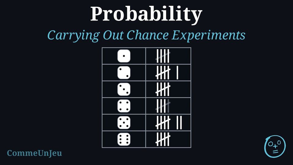
Mia rolls a fair die \(30\) times. What can she predict? Here are her results: compare them with the prediction. | Face | Tally Marks | Total |
| \(1\) |  | 4 |
| \(2\) |  | 6 |
| \(3\) |  | 5 |
| \(4\) |  | 3 |
| \(5\) |  | 7 |
| \(6\) | | 5 |
The six faces of a fair die have the same chance. \(30\) rolls shared equally among \(6\) faces give \(5\) rolls each, because \(6 \times 5 = 30\): Mia can predict about 5 for each face.
Her totals: \(4 + 6 + 5 + 3 + 7 + 5 = 30\), so every roll is counted once. Each total lies between \(3\) and \(7\), close to \(5\), and only two faces came up exactly \(5\) times. The results are close to the prediction without being equal to it, as expected with chance.
Her totals: \(4 + 6 + 5 + 3 + 7 + 5 = 30\), so every roll is counted once. Each total lies between \(3\) and \(7\), close to \(5\), and only two faces came up exactly \(5\) times. The results are close to the prediction without being equal to it, as expected with chance.
So far, we have calculated theoretical probability: a number computed from equally likely outcomes, before any experiment. For example, a fair coin has two equally likely outcomes, heads and tails, so we say \(P(\text{Heads}) = \frac{1}{2}\).
But what if the outcomes are not equally likely? Then counting them does not give the probability. In these cases, we can do an experiment to estimate the probability.
But what if the outcomes are not equally likely? Then counting them does not give the probability. In these cases, we can do an experiment to estimate the probability.
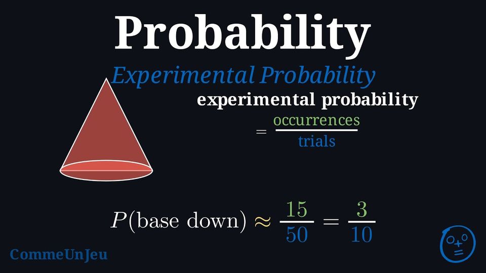
Isaac wants to find the probability that a cone he drops will land on its base. The possible outcomes are “base down” or “on its side”. 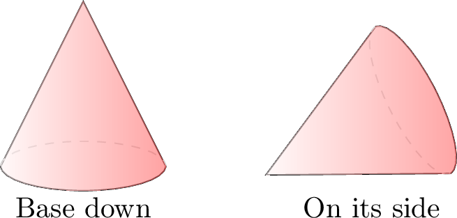
Because of the cone’s shape, nothing says that these two outcomes are equally likely: no symmetry allows us to give them equal probabilities, so a direct calculation is impossible. Isaac therefore estimates the probability by experiment. He tosses the cone 50 times (50 trials) and records the results:
- Base down: 15 times.
- On its side: 35 times.
Definition — Relative Frequency
The relative frequency of an event in a series of trials is the quotient $$ \text{Frequency} = \frac{\text{Number of times the event occurs}}{\text{Total number of trials}} $$ It is a number between \(0\) and \(1\) which describes the series actually observed. When the experiment is repeated many times, this frequency gives an estimate of the probability of the event, also called its experimental probability. In general, the larger the number of trials, the more reliable this estimate is. Skills to practice
- Deciding Whether the Die Has a Memory
- Calculating the Chances at the Next Trial
- Calculating Experimental Probabilities in Percentage Form
- Estimating Probabilities from Experiments
V
Going further
Skills to practice
- Solving Probability Problems
- Quiz
Jump to section