International Baccalaureate · MYP 4
Probability
I
Events and Venn Diagrams
I.1
Events in the Language of Sets
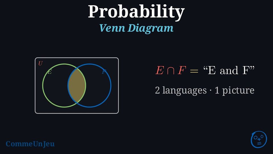
Definition — Set Theory and Probability Vocabulary
| Notation | Set Vocabulary | Probability Vocabulary | Venn Diagram |
| \(U\) | Universal set | Sample space | 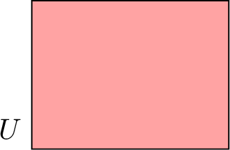 |
| \(x\) | Element of \(U\) | Outcome | 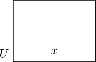 |
| \(\emptyset\) | Empty set | Impossible event | |
| \(E\) | Subset of \(U\) | Event | 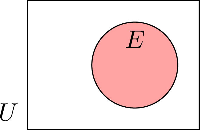 |
| \(x \in E\) | \(x\) is an element of \(E\) | \(x\) is an outcome of \(E\) | 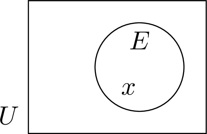 |
| \(E'\) | Complement of \(E\) in \(U\) | Complementary event of \(E\) | 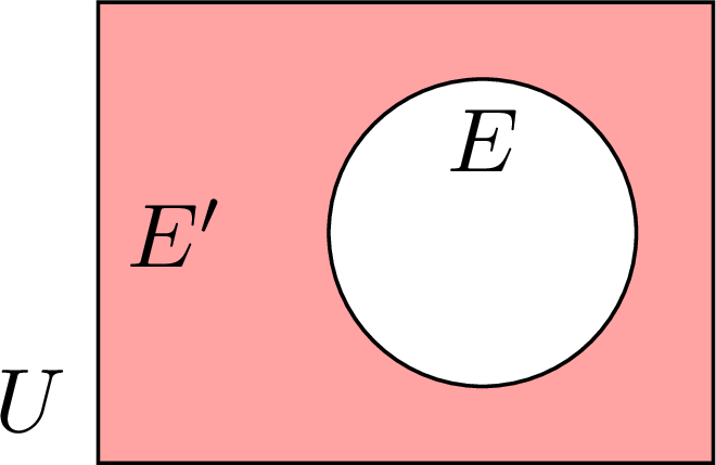 |
| \(E \cup F\) | Union of \(E\) and \(F\) | \(E\) or \(F\) | 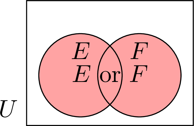 |
| \(E \cap F\) | Intersection of \(E\) and \(F\) | \(E\) and \(F\) | 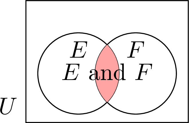 |
| \(E \cap F = \emptyset\) | \(E\) and \(F\) are disjoint | \(E\) and \(F\) are mutually exclusive | 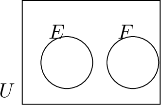 |
Example
One die is rolled: \(U = \{1, 2, 3, 4, 5, 6\}\). Consider the events \(E\): “the result is even” and \(F\): “the result is at least five”. Using the language of sets: - Is \(4 \in E\)? Is \(4 \in F\)?
- Write \(E \cup F\), \(E \cap F\) and \(E'\).
- Are \(E\) and \(F\) mutually exclusive?
Here \(E = \{2, 4, 6\}\) and \(F = \{5, 6\}\).
- \(4\) is even, so \(4 \in E\); but \(4 < 5\), so \(4 \notin F\).
- \(E \cup F = \{2, 4, 5, 6\}\) (in \(E\) or in \(F\)); \(E \cap F = \{6\}\) (in both); \(E' = \{1, 3, 5\}\) (everything else in \(U\)).
- \(E \cap F = \{6\} \neq \varnothing\): the outcome \(6\) realises both events, so \(E\) and \(F\) are not mutually exclusive.
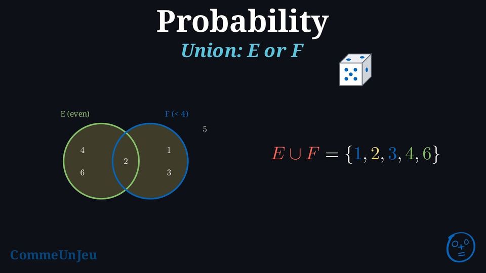
Definition — \(E\) or \(F\)
The union of two events \(E\) and \(F\), denoted \(E \cup F\), is the event that occurs if \(E\) occurs, or \(F\) occurs, or both occur. We read this as “E or F”. It includes all outcomes that are in at least one of the events. Example
A standard six-sided die is rolled. Let event \(E\) be “rolling an even number” and event \(F\) be “rolling a number less than 4”. Find the event \(E \cup F\).
The events are \(E = \{2, 4, 6\}\) and \(F = \{1, 2, 3\}\).
The union \(E \cup F\) contains all outcomes that appear in either set, without repetition: $$ E \cup F = \{1, 2, 3, 4, 6\}. $$
The union \(E \cup F\) contains all outcomes that appear in either set, without repetition: $$ E \cup F = \{1, 2, 3, 4, 6\}. $$
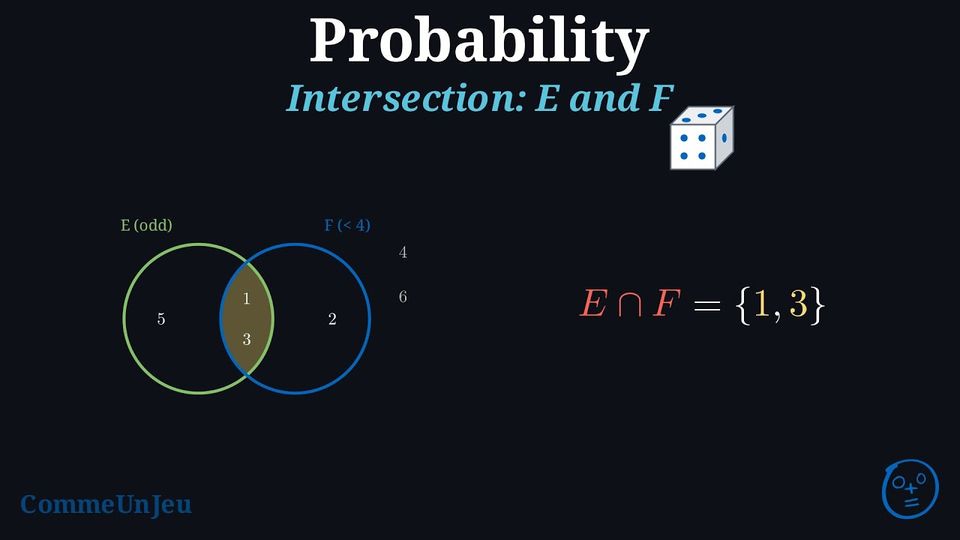
Definition — \(E\) and \(F\)
The intersection of two events \(E\) and \(F\), denoted \(E \cap F\), is the event that occurs if both \(E\) and \(F\) occur simultaneously. We read this as “E and F”. It includes all outcomes that are common to both events. Example
A standard six-sided die is rolled. Let event \(E\) be “rolling an odd number” and event \(F\) be “rolling a number less than 4”. Find the event \(E \cap F\).
The events are \(E = \{1, 3, 5\}\) and \(F = \{1, 2, 3\}\).
The intersection \(E \cap F\) contains only the outcomes that are in both sets: $$ E \cap F = \{1, 3\}. $$
The intersection \(E \cap F\) contains only the outcomes that are in both sets: $$ E \cap F = \{1, 3\}. $$
Skills to practice
- Finding the Union and the Intersection of Two Events
I.2
Probabilities from a Venn Diagram
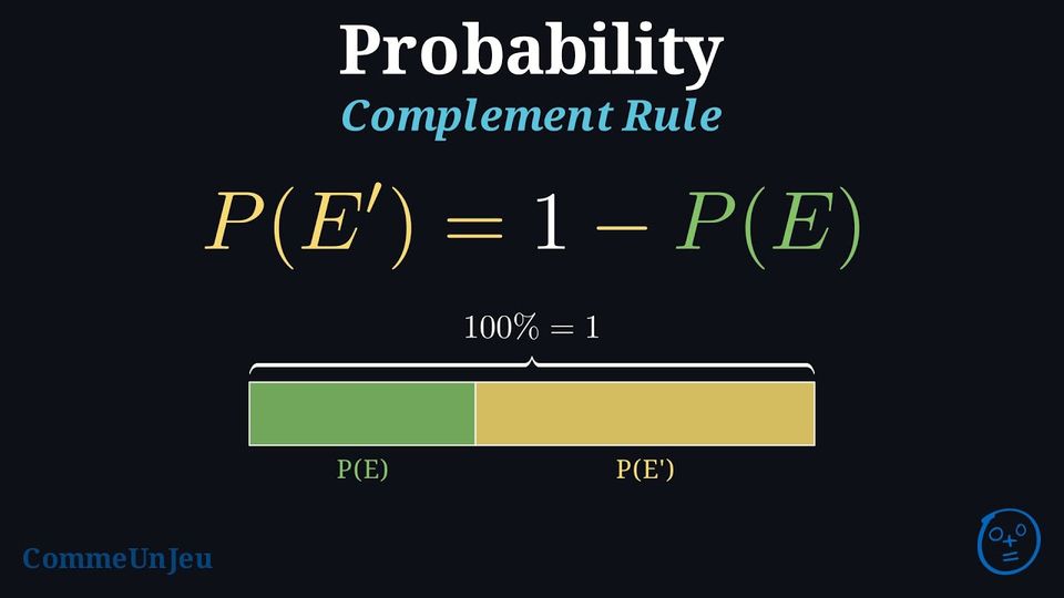
Proposition — Complement Rule
For any event \(E\) and its complementary event \(E'\), their probabilities must add up to \(1\) (or \(100\pourcent\)): $$\textcolor{colorprop}{P(E) + P(E') = 1}$$ This leads to the useful formula for finding the probability of the complement: $$\textcolor{colorprop}{P(E') = 1 - P(E)}$$
The complementary event \(E'\) is made of exactly the outcomes of \(U\) that are not in \(E\). So every outcome of \(U\) lies in exactly one of \(E\) and \(E'\): together they split \(U\) into two parts that overlap nowhere. 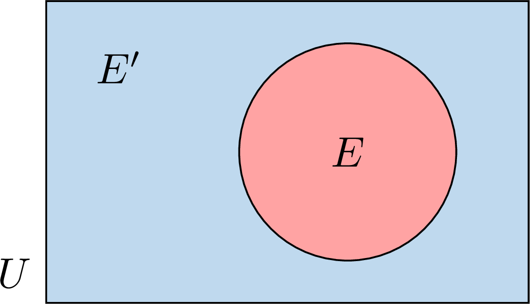
The probability of an event is the sum of the probabilities of its outcomes. Adding \(P(E)\) and \(P(E')\) therefore counts the probability of every outcome of \(U\) exactly once: $$\begin{aligned}[t] P(E) + P(E') &= \text{(sum of the probabilities of all the outcomes of } U\text{)} && \text{(every outcome is in \(E\) or in \(E'\))}\\
&= P(U) && \text{(the whole sample space)}\\
&= 1. \end{aligned}$$ Subtracting \(P(E)\) from both sides gives \(P(E') = 1 - P(E)\).
Method — Finding a Probability from a Venn Diagram
A Venn diagram gives the elements of each region, or their number written in brackets: \((9)\) is a count, a bare \(9\) is an element. The rectangle \(U\) holds the whole group of \(N\) elements. When one element of \(U\) is chosen at random, the \(N\) elements are equally likely, so $$P(\text{event}) = \frac{\text{number of elements in the regions of the event}}{N}.$$ - \(A \cap B\) (“\(A\) and \(B\)”): the overlap of the two circles;
- \(A \cup B\) (“\(A\) or \(B\)”, at least one of the two): every region inside the circles, each counted once;
- “\(A\) only”: the part of the circle \(A\) outside \(B\); “exactly one of the two”: \(A\) only and \(B\) only together;
- \(A'\) (“not \(A\)”): every region outside the circle \(A\); “neither \(A\) nor \(B\)”: the region outside both circles.
Example
In a class of \(32\) pupils, \(14\) swim (\(S\)), \(11\) run (\(R\)) and \(5\) do both. One pupil of the class is chosen at random. - Draw the Venn diagram giving the number of pupils in each region.
- Find the probability that the pupil swims, that the pupil does not swim, that the pupil does both sports, that the pupil does at least one of the two sports, and that the pupil does neither.
- Find the probability that the pupil does exactly one of the two sports.
- Swimming only: \(14 - 5 = 9\); running only: \(11 - 5 = 6\); neither: \(32 - (9 + 5 + 6) = 12\).
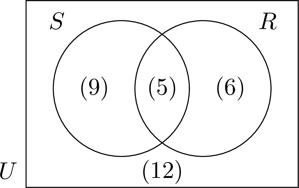
- The \(32\) pupils are equally likely to be chosen. $$\begin{aligned} P(S) &= \frac{9 + 5}{32} = \frac{14}{32} = \frac{7}{16}\\ P(S') &= \frac{6 + 12}{32} = \frac{18}{32} = \frac{9}{16}\\ P(S \cap R) &= \frac{5}{32}\\ P(S \cup R) &= \frac{9 + 5 + 6}{32} = \frac{20}{32} = \frac{5}{8}\\ P(\text{neither}) &= \frac{12}{32} = \frac{3}{8} \end{aligned}$$ “Neither” is the complementary event of “at least one”: \(\dfrac{5}{8} + \dfrac{3}{8} = 1\).
- Exactly one sport: swimming only or running only, \(9 + 6 = 15\) pupils: $$P(\text{exactly one}) = \frac{15}{32}.$$
Skills to practice
- Calculating the Probability of E or F and of E and F
II
Two-Way Tables and Conditional Frequencies
II.1
From Two-Way Tables to Conditional Frequencies
Definition — Two-Way Table of Counts
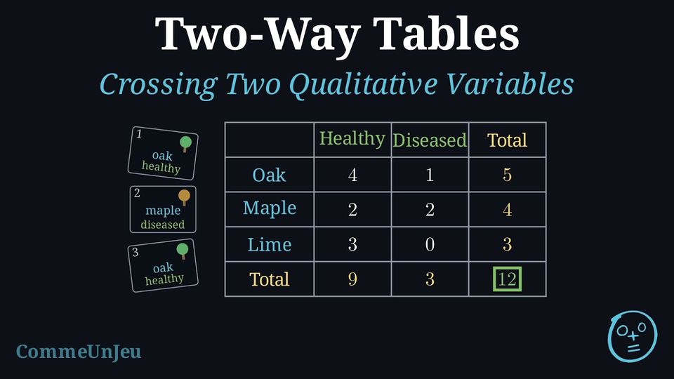
Two qualitative variables are observed on the same population of \(N\) individuals. The two-way table of counts has one row for each category of the first variable and one column for each category of the second; the cell at row \(A\) and column \(B\) holds the count of the individuals that have both categories \(A\) and \(B\), written \(n(A \cap B)\). - The last column holds the row totals: \(n(A)\) is the number of individuals of category \(A\).
- The last row holds the column totals: \(n(B)\) is the number of individuals of category \(B\).
- The bottom-right cell holds the grand total \(N\), which is the sum of the row totals and the sum of the column totals.
Definition — Marginal Frequency
In a two-way table with grand total \(N\), the row and column totals are the marginal counts: they are read in the margins of the table. The marginal frequency of a category \(A\) is the proportion of the whole population that has this category: $$\textcolor{colordef}{f(A) = \frac{n(A)}{N}}.$$ Here the word frequency denotes a proportion, the relative frequency; a number of individuals is a count. Likewise the frequency of a cell is \(\dfrac{n(A \cap B)}{N}\), the proportion of the whole population that has both categories. The marginal frequencies of the categories of one variable add up to \(1\), that is \(100\pourcent\). Example
The \(200\) members of a sports club are sorted by gender and by the sport they practise: | Swimming | Athletics | Total | |
| Women | \(72\) | \(48\) | \(120\) |
| Men | \(32\) | \(48\) | \(80\) |
| Total | \(104\) | \(96\) | \(200\) |
The marginal counts are the totals of the rows and of the columns; each is divided by \(N = 200\): $$\begin{aligned} f(\text{Women}) &= \frac{120}{200} = 0.6, & f(\text{Men}) &= \frac{80}{200} = 0.4, \\
f(\text{Swimming}) &= \frac{104}{200} = 0.52, & f(\text{Athletics}) &= \frac{96}{200} = 0.48. \end{aligned}$$ Check: \(0.6 + 0.4 = 1\) and \(0.52 + 0.48 = 1\). Women are \(60\pourcent\) of the club, and swimming is the sport of \(52\pourcent\) of the members.
Method — Finding a Probability from a Two-Way Table
A two-way table counts the \(N\) individuals of a group by two characteristics. When one individual is chosen at random from the group, the \(N\) individuals are equally likely, so the probability of an event is the number of individuals it counts divided by \(N\), the total in the bottom-right cell: - for one category, use the total of its row or of its column;
- for “\(A\) and \(B\)”, use the cell where the row of \(A\) meets the column of \(B\);
- for “\(A\) or \(B\)” (at least one of the two), add the two totals and subtract the shared cell, whose individuals would otherwise be counted twice;
- for “not \(A\)”, use the complement rule, or the other totals.
Example
A survey asked the \(200\) teenagers of a sports club whether they own a bike. | Bike | No bike | Total | |
| Under \(14\) | \(48\) | \(42\) | \(90\) |
| \(14\) and over | \(72\) | \(38\) | \(110\) |
| Total | \(120\) | \(80\) | \(200\) |
- owns a bike;
- does not own a bike;
- is under \(14\) and owns a bike;
- is under \(14\) or owns a bike.
The \(200\) teenagers are equally likely to be chosen.
- The column “Bike” has the total \(120\): $$P(\text{bike}) = \frac{120}{200} = \frac{3}{5}.$$
- By the complement rule, or with the total \(80\) of the column “No bike”: $$P(\text{no bike}) = 1 - \frac{3}{5} = \frac{2}{5} = \frac{80}{200}.$$
- The cell where the row “Under \(14\)” meets the column “Bike” holds \(48\): $$P(\text{under } 14 \text{ and bike}) = \frac{48}{200} = \frac{6}{25}.$$
- The row “Under \(14\)” counts \(90\) teenagers and the column “Bike” \(120\); the \(48\) teenagers of the shared cell are in both, so they are subtracted once: $$\begin{aligned} P(\text{under } 14 \text{ or bike}) &= \frac{90 + 120 - 48}{200}\\ &= \frac{162}{200}\\ &= \frac{81}{100} \end{aligned}$$ Check: the teenagers who are neither under \(14\) nor bike owners are the \(38\) of the cell “\(14\) and over, No bike”, and \(\frac{200 - 38}{200} = \frac{162}{200}\).
Definition — Conditional Frequency
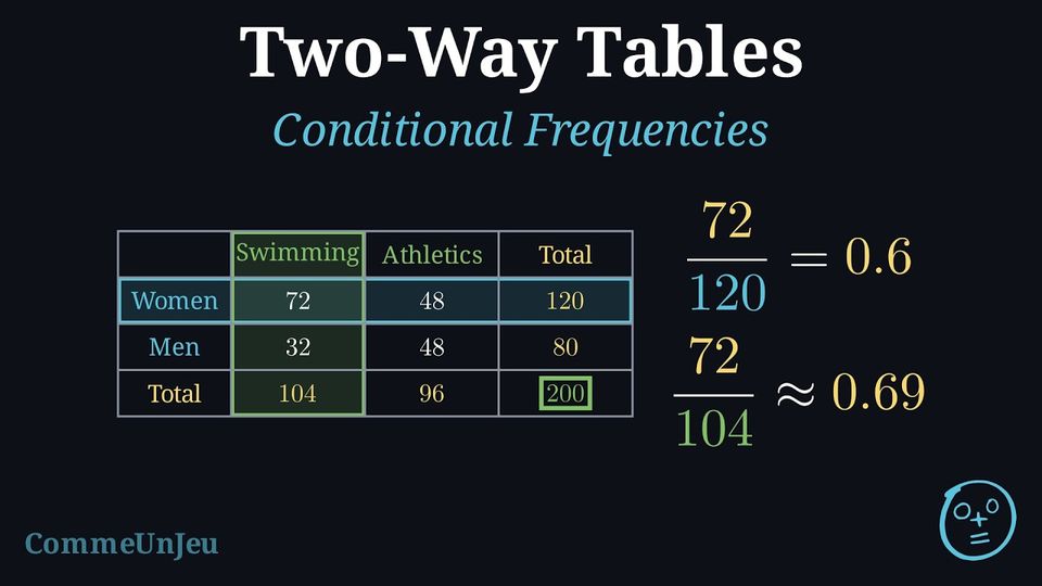
The conditional frequency of a category \(B\) given a category \(A\) observed at least once (\(n(A) > 0\)) is the proportion of the individuals of \(A\) that also have \(B\): $$\textcolor{colordef}{f_A(B) = \frac{n(A \cap B)}{n(A)}}.$$ It is computed inside the sub-population \(A\): the numerator is the cell at row \(A\) and column \(B\), the denominator is the marginal count of \(A\), not the grand total. The conditional frequencies given \(A\) of all the categories of the other variable add up to \(1\). Method — Row Profiles and Column Profiles
To compare the groups defined by one variable: - Choose the variable that defines the groups: its categories are the rows (or the columns) of the table.
- Divide each cell of a row by the total of that row (a row observed at least once): the row now reads as conditional frequencies, its row profile — the list of the \(f_A(B)\) for the category \(A\) of that row — which adds up to \(1\).
- Compare the profiles row by row: two groups with the same profile are distributed alike over the other variable.
Example
In the sports club of \(200\) members (women \(72\) swimmers and \(48\) athletes, men \(32\) swimmers and \(48\) athletes): - Compute the frequency of swimming among the women and among the men. Do the two groups practise the same sports in the same proportions?
- Compute the frequency of women among the swimmers and among the athletes.
- The groups are the rows. Each cell is divided by its row total: $$\begin{aligned} f_{\text{Women}}(\text{Swimming}) &= \frac{n(\text{Women} \cap \text{Swimming})}{n(\text{Women})} = \frac{72}{120} = 0.6, \\ f_{\text{Men}}(\text{Swimming}) &= \frac{n(\text{Men} \cap \text{Swimming})}{n(\text{Men})} = \frac{32}{80} = 0.4. \end{aligned}$$ The row profiles are \((0.6\,;\,0.4)\) for the women and \((0.4\,;\,0.6)\) for the men: \(60\pourcent\) of the women swim, against \(40\pourcent\) of the men. The two groups do not practise the sports in the same proportions.
- The groups are now the columns. Each cell is divided by its column total: $$\begin{aligned} f_{\text{Swimming}}(\text{Women}) &= \frac{72}{104} = \frac{9}{13} \approx 0.69, \\ f_{\text{Athletics}}(\text{Women}) &= \frac{48}{96} = 0.5. \end{aligned}$$ About \(69\pourcent\) of the swimmers are women, and exactly half of the athletes. Note that \(f_{\text{Women}}(\text{Swimming}) = 0.6\) and \(f_{\text{Swimming}}(\text{Women}) \approx 0.69\) share the numerator \(72\) but not the denominator: “\(60\pourcent\) of the women swim” and “\(69\pourcent\) of the swimmers are women” are two different facts.
Reading a Sentence
A sentence about a two-way table names a frequency, and the words tell which one. “\(60\pourcent\) of the women swim”: the population is restricted to the women, then the swimmers are counted among them — a conditional frequency, \(f_{\text{Women}}(\text{Swimming})\). “\(36\pourcent\) of the members are women who swim”: the population is the whole club and the category is “woman and swimmer” — the frequency of a cell, \(\frac{72}{200}\). “\(52\pourcent\) of the members swim”: a marginal frequency, \(f(\text{Swimming})\). The words of the, among, out of introduce the group that serves as the denominator. Many sentences in the media are true and yet misread, because the reader takes a column profile for a row profile: “most of the swimmers are women” does not mean that most women swim. In a club where \(40\) of the \(100\) women and \(10\) of the \(100\) men swim, \(80\pourcent\) of the swimmers are women, while only \(40\pourcent\) of the women swim.
Skills to practice
- Reading a Sentence
- Computing Conditional Frequencies
- Comparing Row Profiles
III
Tree Diagrams
III.1
Independent Events and Tree Diagrams
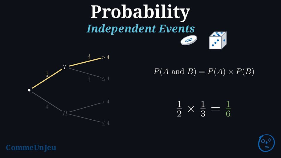
Independent events are events where knowing that one event has happened does not change the probability that the other event happens. For example, when rolling two fair dice at the same time, the result of the first die does not change the chances for the second die — they are independent events.
Definition — Independent Events
Two events \(A\) and \(B\) are independent when the probability that both happen (that is, \(P(A\cap B)\) or \(P(A \text{ and } B)\)) is the product of their individual probabilities. This is called the multiplication rule for independent events: $$P(A \text{ and } B) = P(A) \times P(B)$$ Example
An experiment consists of the following two independent actions: - Tossing a fair coin.
- Rolling a fair six-sided die.
Let \(T\) be the event “getting tails” and \(N\) be the event “rolling a number greater than 4”.
- The events are independent, so we can use the multiplication rule.
- The probability of getting tails is \(P(T) = \dfrac{1}{2}\).
- The outcomes for a number greater than 4 are \(\{5, 6\}\). There are 2 favourable outcomes out of 6 total outcomes. So, \(P(N) = \dfrac{2}{6} = \dfrac{1}{3}\).
- Now, we multiply the probabilities to find the probability of both events happening: $$\begin{aligned} P(T \text{ and } N) &= P(T) \times P(N) \\ &= \dfrac{1}{2} \times \dfrac{1}{3} \\ &= \dfrac{1}{6} \end{aligned}$$
Method — Using a Probability Tree Diagram
- Draw branches for each step: Draw branches for the first event (coin toss) and then, from the end of each of those branches, draw the branches for the second event (die roll).
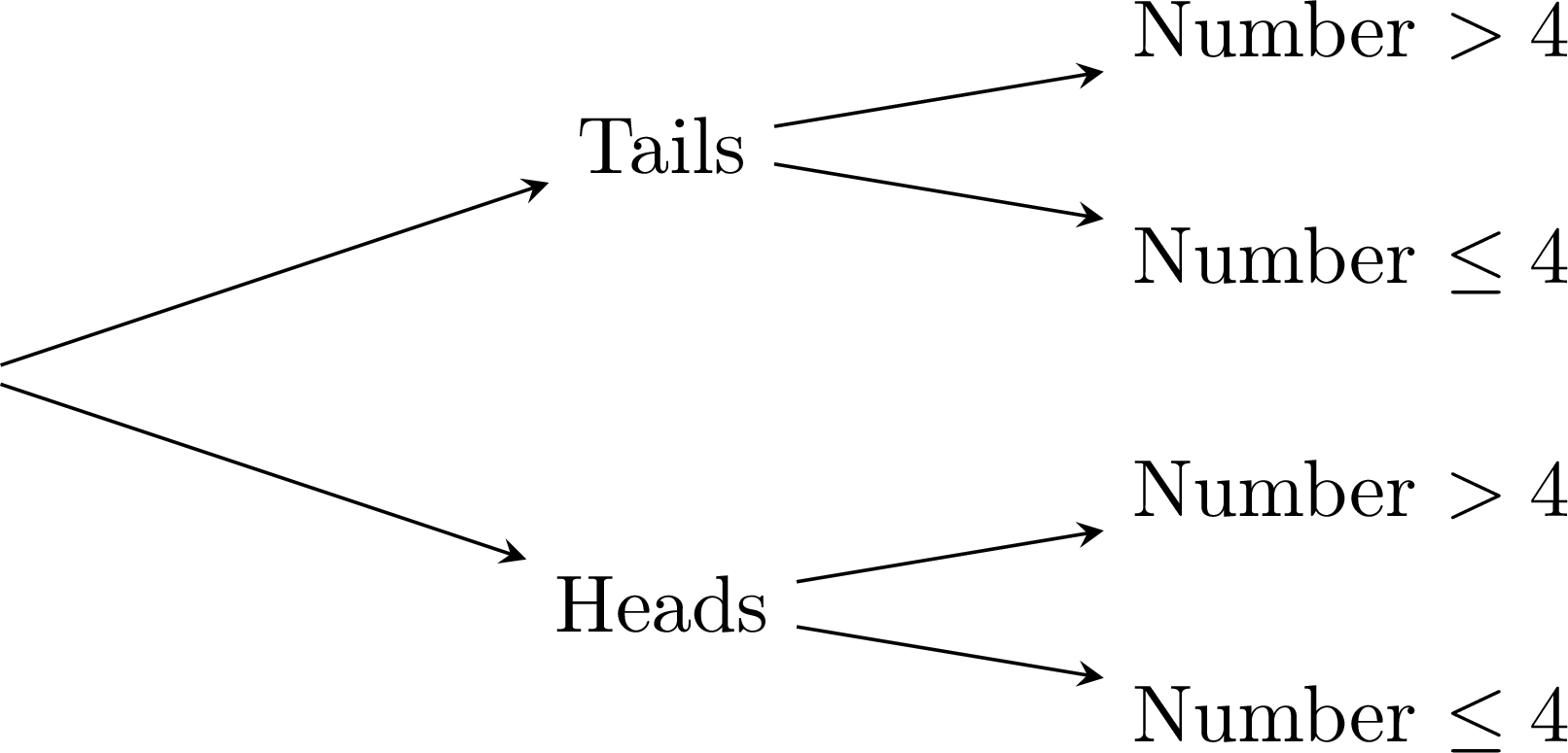
- Write probabilities on each branch: The probabilities on the branches from a single point must add up to 1. Because the events are independent, the probabilities on the die-roll branches are the same after “Tails” and after “Heads”.
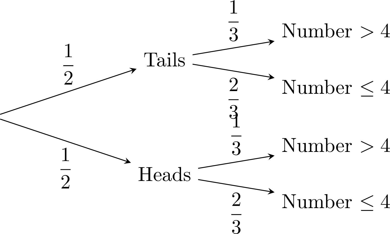
- Multiply along the path: To find the probability of a combined event, multiply the probabilities along the path from start to finish.
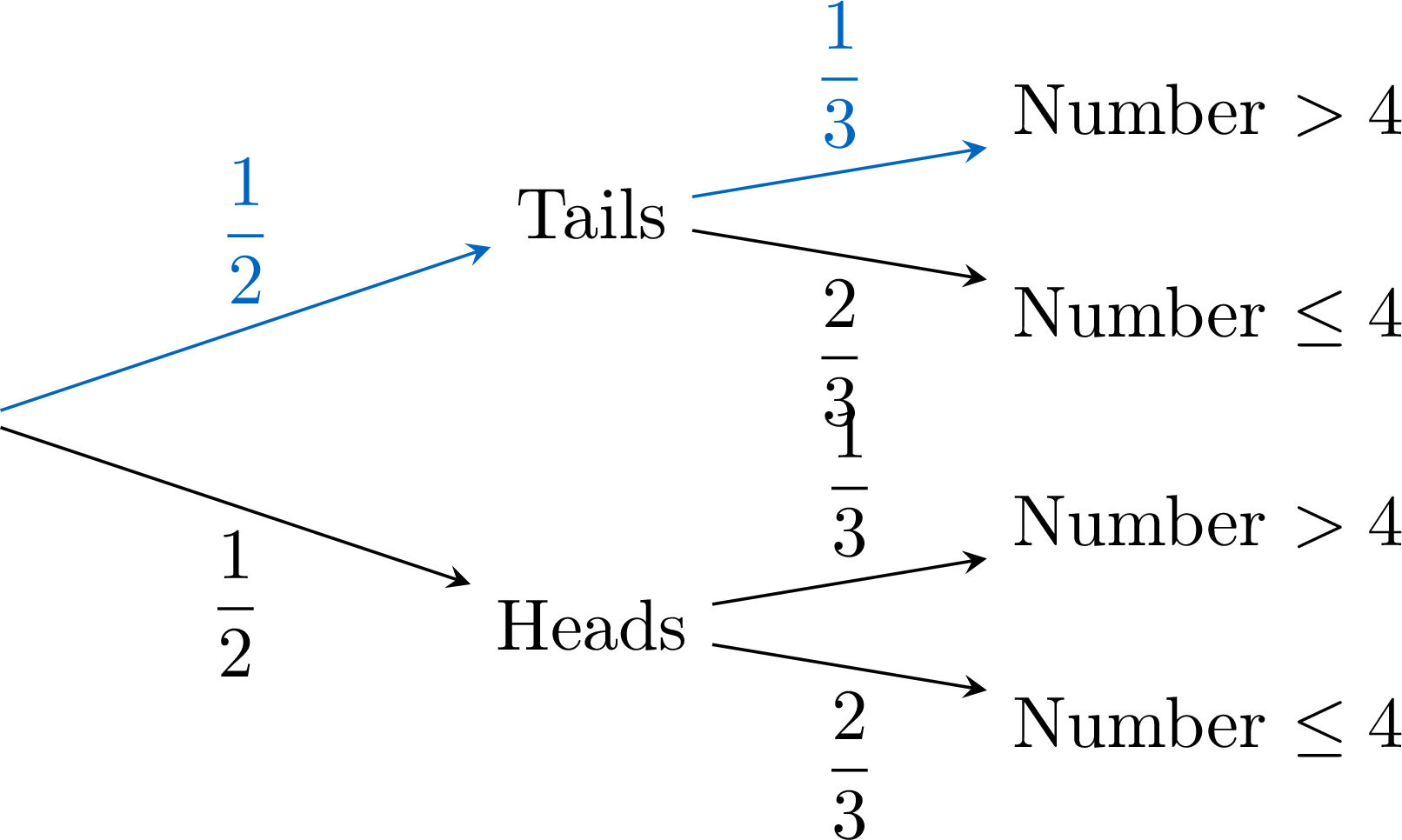 $$\textcolor{colorprop}{P(\text{``Tails'' and ``Number > 4''})=\frac{1}{2}\times \frac{1}{3}}$$
Skills to practice
- Counting the Outcomes in a Tree Diagram
- Completing a Probability Tree Diagram
- Calculating Probabilities from a Tree Diagram
- Drawing a Probability Tree for Two Independent Events
IV
Dependent Events
IV.1
Drawing without Replacement
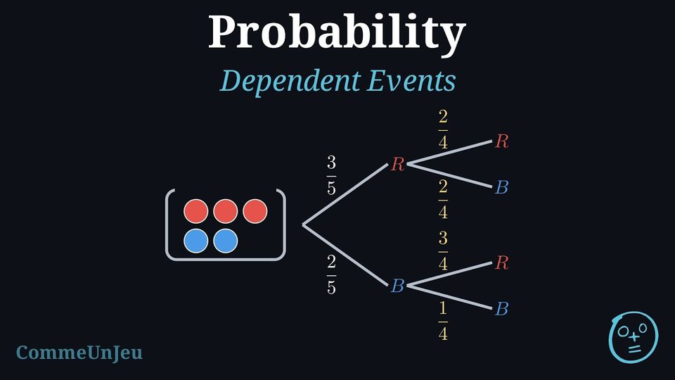
With or Without Replacement
A bag holds three red marbles and two blue marbles, identical to the touch. A marble is drawn and its colour is noted, then a second marble is drawn. 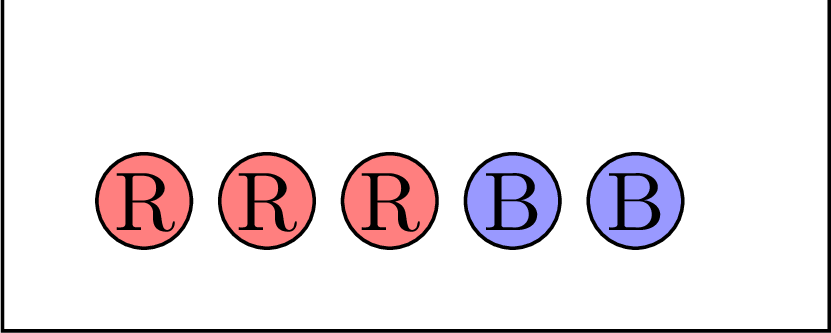
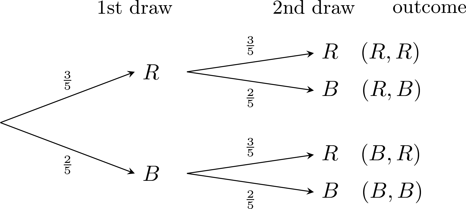
- With replacement, the first marble is put back before the second draw. The bag is the same for both draws: the second marble is red with probability \(\frac{3}{5}\) and blue with probability \(\frac{2}{5}\), whatever the colour of the first one. The second level of the tree carries the same fractions after \(R\) and after \(B\): the two draws are independent, and \(P(\text{red, then red}) = \frac{3}{5} \times \frac{3}{5} = \frac{9}{25}\).
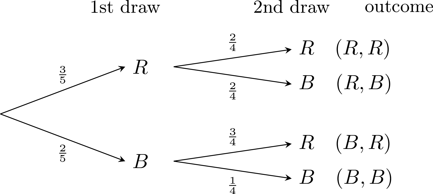
- Without replacement, the first marble stays out: the second marble is drawn from the \(4\) marbles left, and what is left depends on the first colour. After a red marble, \(2\) red and \(2\) blue marbles remain, so the second is red with probability \(\frac{2}{4}\); after a blue marble, \(3\) red and \(1\) blue remain, so the second is red with probability \(\frac{3}{4}\). The fractions of the second level change with the first result: the two draws are dependent, and \(P(\text{red, then red}) = \frac{3}{5} \times \frac{2}{4} = \frac{3}{10}\).
Definition — Dependent Events
Objects are drawn with replacement when each object drawn is put back before the next draw, and without replacement when it is kept out.Two events are dependent when they are not independent: knowing that one of them has happened changes the probability of the other. Draws without replacement are the typical case: the first draw changes what is left for the second one.
Method — Using a Tree for Dependent Events
- Draw the tree, one level per step, as for independent events, and write the probabilities of the first step on the first level.
- Second level: after each result of the first step, write the probabilities of the second step once that result has happened. For draws without replacement, recount what is left: one object fewer in all, and one fewer of the kind already drawn. The probabilities on the branches leaving a point still add up to \(1\).
- Multiply along a path: the probability that \(A\) happens, then \(B\), is $$\textcolor{colorprop}{P(A \text{ then } B) = P(A) \times P(B \text{ once } A \text{ has happened})}.$$
- Add the paths: when several paths give the event, add their probabilities. The probabilities of all the paths add up to \(1\), which gives a check.
Example
A bag holds \(3\) red marbles and \(2\) blue marbles, identical to the touch. Two marbles are drawn one after the other, without replacement. - Draw the probability tree.
- Calculate the probability that both marbles are red.
- Calculate the probability that the two marbles have different colours.
- Calculate the probability that the second marble is red, and compare with draws with replacement.
Write \(R\) for a red marble and \(B\) for a blue one, in the order of the draws.
- First draw: \(3\) red out of \(5\) marbles. After a red marble, \(2\) red and \(2\) blue remain; after a blue marble, \(3\) red and \(1\) blue remain. Each path ends with its probability, the product along it:
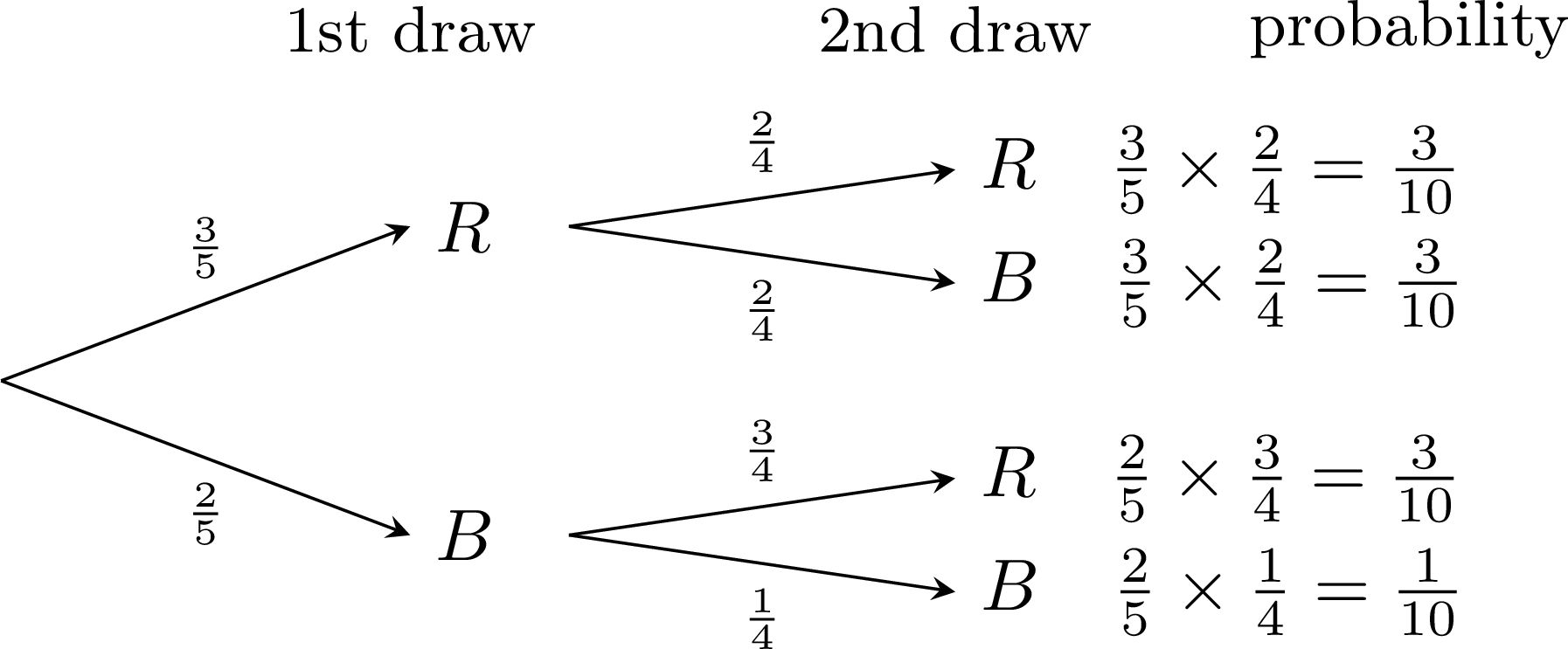
- Both red is the path \(R\) then \(R\): $$\begin{aligned}[t] P(R \text{ then } R) &= P(R) \times P(R \text{ once } R \text{ has happened}) && \text{(multiply along the path)}\\ &= \frac{3}{5} \times \frac{2}{4}\\ &= \frac{6}{20} = \frac{3}{10}. \end{aligned}$$ Check by counting: the first marble can be any of \(5\) and the second any of the \(4\) left, so there are \(5 \times 4 = 20\) equally likely ordered draws, of which \(3 \times 2 = 6\) are red then red: \(\frac{6}{20} = \frac{3}{10}\). The product along the path is exactly this fraction of the ordered draws.
- Different colours are the paths \(R\) then \(B\), and \(B\) then \(R\): $$\begin{aligned}[t] P(\text{different colours}) &= \frac{3}{5} \times \frac{2}{4} + \frac{2}{5} \times \frac{3}{4} && \text{(add the two paths)}\\ &= \frac{3}{10} + \frac{3}{10}\\ &= \frac{3}{5}. \end{aligned}$$
- The second marble is red on the paths \(R\) then \(R\), and \(B\) then \(R\): $$\begin{aligned}[t] P(\text{second marble red}) &= \frac{3}{5} \times \frac{2}{4} + \frac{2}{5} \times \frac{3}{4} && \text{(add the two paths)}\\ &= \frac{3}{10} + \frac{3}{10}\\ &= \frac{3}{5}. \end{aligned}$$ With replacement, the second marble is red with probability \(\frac{3}{5}\) on every branch. The value is the same, for a different reason: without replacement, the chance of red on the second draw is \(\frac{2}{4}\) or \(\frac{3}{4}\) depending on the first marble, and the two cases balance out. The draws are still dependent: knowing the first colour changes the probability of the second.
Example
Two cards are drawn one after the other, without replacement, from a standard pack of \(52\) cards, \(13\) of which are hearts. Let \(H_1\) be the event “the first card is a heart” and \(H_2\) the event “the second card is a heart”. - Draw the probability tree.
- Calculate the probability that both cards are hearts.
- Calculate the probability that at least one of the two cards is a heart.
- First draw: \(13\) hearts out of \(52\) cards. After a heart, \(12\) hearts remain among \(51\) cards; after another card, the \(13\) hearts remain among \(51\) cards.
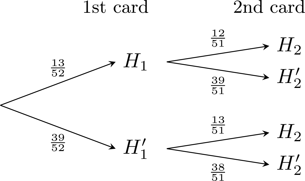
- Both hearts is the path \(H_1\) then \(H_2\): $$\begin{aligned}[t] P(H_1 \text{ then } H_2) &= \frac{13}{52} \times \frac{12}{51} && \text{(multiply along the path)}\\ &= \frac{1}{4} \times \frac{12}{51}\\ &= \frac{12}{204} = \frac{1}{17}. \end{aligned}$$
- “At least one heart” is the complementary event of “no heart”, which is the single path \(H_1'\) then \(H_2'\): $$\begin{aligned}[t] P(\text{at least one heart}) &= 1 - P(H_1' \text{ then } H_2') && \text{(complement rule)}\\ &= 1 - \frac{39}{52} \times \frac{38}{51} && \text{(multiply along the path)}\\ &= 1 - \frac{3}{4} \times \frac{38}{51}\\ &= 1 - \frac{19}{34}\\ &= \frac{15}{34}. \end{aligned}$$ Adding the three paths that contain a heart gives the same value: \(\frac{1}{17} + \frac{13}{68} + \frac{13}{68} = \frac{4}{68} + \frac{26}{68} = \frac{30}{68} = \frac{15}{34}\).
Example
A club has \(4\) girls and \(3\) boys. Two captains are chosen at random, one after the other: the first from the \(7\) members, the second from the \(6\) members left. Calculate the probability that - both captains are girls;
- the captains are one girl and one boy.
Write \(G\) for a girl and \(B\) for a boy. The second captain is chosen from the \(6\) members left, so the second level depends on the first choice: 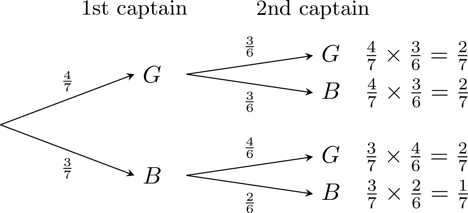
- Both girls is the path \(G\) then \(G\): $$\begin{aligned}[t] P(G \text{ then } G) &= \frac{4}{7} \times \frac{3}{6} && \text{(multiply along the path)}\\ &= \frac{12}{42} = \frac{2}{7}. \end{aligned}$$
- One girl and one boy are the paths \(G\) then \(B\), and \(B\) then \(G\): $$\begin{aligned}[t] P(\text{one girl and one boy}) &= \frac{4}{7} \times \frac{3}{6} + \frac{3}{7} \times \frac{4}{6} && \text{(add the two paths)}\\ &= \frac{12}{42} + \frac{12}{42}\\ &= \frac{24}{42} = \frac{4}{7}. \end{aligned}$$
Skills to practice
- Recognising Dependent Draws
- Finding the Probability of the Second Draw
- Completing a Tree for Draws without Replacement
- Calculating Probabilities of Dependent Events
- Solving Problems with Dependent Events
V
Expected Gain, Fair Games and Simulation
V.1
Expected Count, Expected Gain and Simulation
Proposition — Fluctuation and Stabilisation
An experiment is repeated \(n\) times under the same conditions, each repetition having no influence on the others, and the frequency of an event of probability \(p\) is observed. - Fluctuation: for a fixed \(n\), the frequency can change from one series to another. Two series of the same length do not necessarily give the same frequency.
- Stabilisation: when \(n\) grows, the frequencies tend to move closer to \(p\). Long series usually stray less from \(p\) than short ones.
- Expected count: over \(n\) repetitions, the expected count of the event is \(n \times p\); the observed count is about \(n \times p\), in the sense that the observed frequency, the count divided by \(n\), is usually close to \(p\). “About”: the observed count is not known in advance, and it need not equal \(n \times p\) exactly.
Example
Two pupils each throw a fair die again and again, and record the frequency of “getting a \(6\)” as the number \(n\) of throws grows (the \(n\)-axis is not drawn to scale). 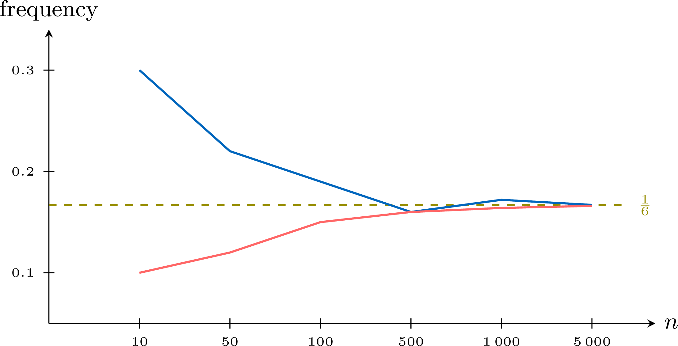
- For which values of \(n\) do the two frequencies differ the most? What is this phenomenon called?
- Around which value do the two curves settle? Why?
- How many sixes are expected over \(1\,200\) throws?
- After \(600\) throws, one pupil has only \(85\) sixes instead of the \(100\) expected. Will the following throws “make up” for it?
- For the small values of \(n\): at \(n = 10\) the frequencies are \(0.30\) and \(0.10\). This is the fluctuation: short series differ a lot from one another.
- Both curves settle around \(\dfrac{1}{6} \approx 0.167\), the probability of getting a \(6\) with a fair die. This is the stabilisation: the longer the series, the closer its frequency is to the probability.
- \(1\,200 \times \dfrac{1}{6} = \textcolor{colordef}{200}\): about \(200\) sixes are expected — a real series will give a number close to \(200\), without \(200\) itself being guaranteed.
- No. The die has no memory: each throw still has a probability \(\dfrac{1}{6}\) of giving a \(6\). The frequency comes close to \(\dfrac{1}{6}\) because the \(15\) missing sixes weigh less and less among more and more throws — they are diluted, not made up for.
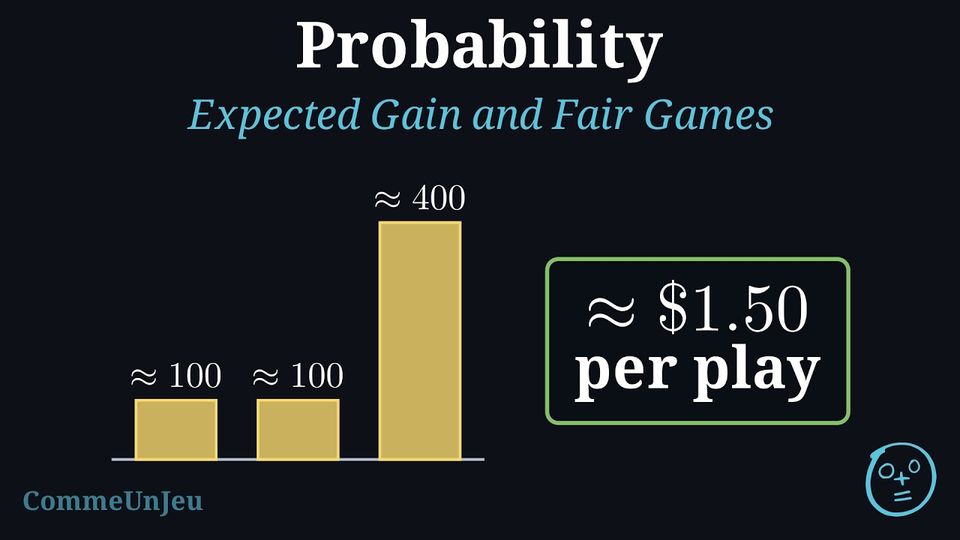
A game of chance has a price to play and prizes. Knowing the probability of winning is not enough to decide whether it is worth playing: a likely win of a small prize can be worth less than the price, and an unlikely win of a large prize can be worth more. What matters is how much each result pays and how often it happens.
Definition — Expected Gain
The possible gains of a game are \(g_1\), \(g_2\), …, \(g_k\) (a gain of \(0\) for a result that pays nothing), with probabilities \(p_1\), \(p_2\), …, \(p_k\). The expected gain of one play, also called the expected return, is $$\textcolor{colordef}{g_1 \times p_1 + g_2 \times p_2 + \dots + g_k \times p_k}.$$
Why the Expected Gain Is an Average
Over a large number \(n\) of plays, the gain \(g_1\) is expected about \(n \times p_1\) times, the gain \(g_2\) about \(n \times p_2\) times, and so on: these are the expected counts. The total gain of the \(n\) plays is therefore about \(g_1 \times n p_1 + g_2 \times n p_2 + \dots + g_k \times n p_k\), and dividing by \(n\) gives the average gain per play: $$\text{average gain per play} \approx \frac{g_1 \times n p_1 + \dots + g_k \times n p_k}{n} = g_1 \times p_1 + \dots + g_k \times p_k.$$ The expected gain is the average gain per play in the long run. A single play does not pay it in general: it pays one of the gains \(g_1\), …, \(g_k\).
Definition — Net Expected Gain and Fair Game
When one play costs a price \(m\) (the stake), the net expected gain of one play is $$\textcolor{colordef}{\text{expected gain} - m}.$$ The game is fair when its net expected gain is \(0\), that is when the price equals the expected gain. When the net expected gain is greater than \(0\), the game favours the player; when it is less than \(0\), it favours the organiser, who keeps about \(m - \text{expected gain}\) per play in the long run. Method — Deciding Whether a Game Is Worth Playing
- List the possible gains and their probabilities in a table, and check that the probabilities add up to \(1\).
- Calculate the expected gain: the sum of the products gain \(\times\) probability.
- Subtract the price to play: this gives the net expected gain. The same value is obtained by working directly with the net gain of each result (prize minus price), because the probabilities add up to \(1\).
- Conclude: greater than \(0\), the game favours the player; equal to \(0\), it is fair; less than \(0\), it favours the organiser. The fair price is the expected gain.
Example
A fair six-sided die is rolled. The player receives \(\dollar 6\) for a \(6\), \(\dollar 3\) for a \(5\), and nothing otherwise. - Calculate the expected gain of one play.
- What price to play makes the game fair?
- The organiser charges \(\dollar 2\) per play. Calculate the net expected gain and conclude.
The six faces are equally likely. The gains and their probabilities:
| result | \(6\) | \(5\) | \(1\), \(2\), \(3\) or \(4\) |
| gain (\dollar) | \(6\) | \(3\) | \(0\) |
| probability | \(\frac{1}{6}\) | \(\frac{1}{6}\) | \(\frac{4}{6}\) |
- $$\begin{aligned}[t] \text{expected gain} &= 6 \times \frac{1}{6} + 3 \times \frac{1}{6} + 0 \times \frac{4}{6} && \text{(definition of the expected gain)}\\ &= 1 + \frac{1}{2} + 0\\ &= 1.5. \end{aligned}$$ On average, one play pays \(\dollar 1.50\).
- The game is fair when the price equals the expected gain: a price of \(\dollar 1.50\).
- $$\begin{aligned}[t] \text{net expected gain} &= \text{expected gain} - m && \text{(definition)}\\ &= 1.5 - 2\\ &= -0.5. \end{aligned}$$ The net expected gain is less than \(0\): the game favours the organiser. Over many plays the player loses about \(\dollar 0.50\) per play, for instance about \(\dollar 50\) over \(100\) plays.
Example
A school sells \(500\) raffle tickets at \(\dollar 2\) each. One ticket wins a prize of \(\dollar 300\), two tickets win \(\dollar 100\) each, and five tickets win \(\dollar 20\) each; the other tickets win nothing, and every ticket has the same chance. Sam buys one ticket. - Make the table of Sam's possible gains and their probabilities.
- Calculate the expected gain of the ticket, then its net expected gain.
- How much money does the raffle raise for the school once all the tickets are sold?
- \(1 + 2 + 5 = 8\) tickets win, so \(500 - 8 = 492\) tickets win nothing.
gain (\dollar) \(300\) \(100\) \(20\) \(0\) probability \(\frac{1}{500}\) \(\frac{2}{500}\) \(\frac{5}{500}\) \(\frac{492}{500}\) - The expected gain of the ticket, then its net expected gain: $$\begin{aligned}[t] \text{expected gain} &= 300 \times \frac{1}{500} + 100 \times \frac{2}{500} + 20 \times \frac{5}{500} + 0 \times \frac{492}{500} && \text{(definition)}\\ &= \frac{300 + 200 + 100}{500}\\ &= \frac{600}{500} = 1.2. \end{aligned}$$ $$\begin{aligned}[t] \text{net expected gain} &= 1.2 - 2 && \text{(price } m = 2\text{)}\\ &= -0.8. \end{aligned}$$ A ticket pays back \(\dollar 1.20\) on average: Sam loses \(\dollar 0.80\) on average.
- The school collects \(500 \times 2 = \dollar 1\,000\) and pays out \(300 + 2 \times 100 + 5 \times 20 = \dollar 600\) of prizes, so it raises \(1\,000 - 600 = \dollar 400\). This is \(500 \times 0.80\): the \(\dollar 0.80\) each ticket loses on average, times the number of tickets.
Example
At a fairground stall, a player pays \(\dollar 2\) and spins a fair spinner with \(8\) equal sectors: \(1\) sector pays \(\dollar 10\), \(2\) sectors pay \(\dollar 2\), and the other \(5\) sectors pay nothing. 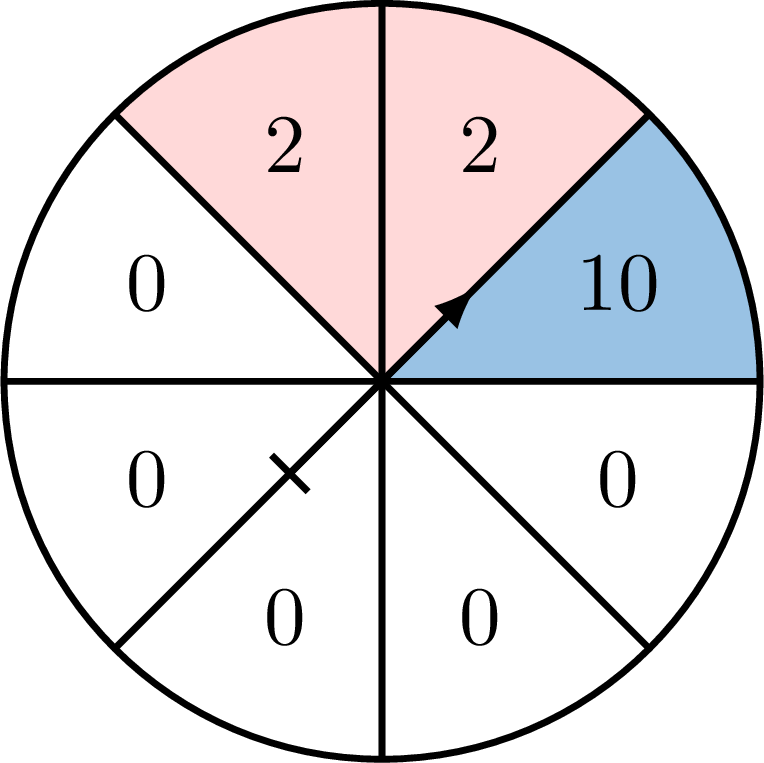
- Calculate the net expected gain of one play, first with the prizes, then with the net gain of each result.
- The stall owner expects \(400\) plays in an evening. How much can she expect to earn?
- The \(8\) sectors are equally likely, so the prizes \(10\), \(2\) and \(0\) have probabilities \(\frac{1}{8}\), \(\frac{2}{8}\) and \(\frac{5}{8}\). $$\begin{aligned}[t] \text{expected gain} &= 10 \times \frac{1}{8} + 2 \times \frac{2}{8} + 0 \times \frac{5}{8} && \text{(definition)}\\
&= \frac{10 + 4}{8}\\
&= \frac{14}{8} = 1.75, \end{aligned}$$ so the net expected gain is \(1.75 - 2 = -0.25\).
With the net gains: the player ends \(10 - 2 = 8\) up, \(2 - 2 = 0\) (the price back), or \(0 - 2 = -2\), that is \(2\) down: $$\begin{aligned}[t] \text{net expected gain} &= 8 \times \frac{1}{8} + 0 \times \frac{2}{8} + (-2) \times \frac{5}{8} && \text{(net gains)}\\ &= \frac{8 - 10}{8}\\ &= -\frac{2}{8} = -0.25. \end{aligned}$$ The two ways agree: subtracting \(2\) from every gain subtracts \(2 \times \bigl(\frac{1}{8} + \frac{2}{8} + \frac{5}{8}\bigr) = 2\) from the sum. The game favours the stall. - Each play leaves the stall about \(\dollar 0.25\) on average, so over \(400\) plays she can expect about \(400 \times 0.25 = \dollar 100\) — an estimate, not a certainty.
The Problem of Points
In \(1654\), Pascal and Fermat were asked how to share the stakes of a game of chance stopped before its end. Their answer gives each player the pot multiplied by that player's probability of winning it, had the game gone on: exactly the player's expected gain from continuing to play, since the pot is won with that probability and nothing is won otherwise. This problem is one of the starting points of the idea of expected gain.
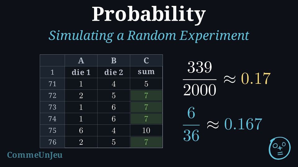
Estimating a probability by experiment requires a large number of trials — and rolling a die ten thousand times is out of reach. The way round is to replace the experiment by another one that behaves in the same way but can be repeated very quickly: a simulation.
Method — Simulating a Random Experiment
To simulate an experiment is to replace it by another one, quicker to repeat, in which each outcome of the original experiment is coded by one or several outcomes of the model — with the same probabilities. - Choose the model and state the coding: a fair coin for two equally likely outcomes; a fair six-sided die, where “even” and “odd” also code two equally likely outcomes; numbered tokens or a spinner otherwise.
- Or use a spreadsheet:
=RANDBETWEEN(1,6)returns a whole number between \(1\) and \(6\), each with the same probability; copying the cell down simulates as many trials as needed. - Repeat a large number of times and count how often the studied event occurs.
- Read its frequency: it estimates the probability, all the more reliably as the number of trials is large.
Example
Two fair dice are rolled and their results are added. We want to estimate the probability of the event \(S\): “the sum is \(7\)”. - Which spreadsheet formulas simulate one roll of the two dice?
- A simulation of \(2\,000\) such rolls gives \(339\) sums equal to \(7\). Estimate \(P(S)\).
- The table below gives the \(36\) equally likely outcomes of this two-step experiment. Compute \(P(S)\) exactly and compare.
| \(+\) | \(1\) | \(2\) | \(3\) | \(4\) | \(5\) | \(6\) |
| \(1\) | \(2\) | \(3\) | \(4\) | \(5\) | \(6\) | \(7\) |
| \(2\) | \(3\) | \(4\) | \(5\) | \(6\) | \(7\) | \(8\) |
| \(3\) | \(4\) | \(5\) | \(6\) | \(7\) | \(8\) | \(9\) |
| \(4\) | \(5\) | \(6\) | \(7\) | \(8\) | \(9\) | \(10\) |
| \(5\) | \(6\) | \(7\) | \(8\) | \(9\) | \(10\) | \(11\) |
| \(6\) | \(7\) | \(8\) | \(9\) | \(10\) | \(11\) | \(12\) |
- One cell with
=RANDBETWEEN(1,6)for the first die, a second cell with=RANDBETWEEN(1,6)for the second one, and a third cell adding the two. - The frequency of \(S\) is $$\dfrac{339}{2\,000} = 0{.}1695,$$ so \(P(S) \approx 0{.}17\).
- The table shows \(6\) cells equal to \(7\) (the diagonal \(1+6\), \(2+5\), \(3+4\), \(4+3\), \(5+2\), \(6+1\)) out of \(36\) equally likely outcomes: $$P(S) = \dfrac{6}{36} = \dfrac{1}{6} \approx 0{.}167.$$ The simulated frequency \(0{.}1695\) is very close to it, as expected for a large number of trials.
Skills to practice
- Deciding Whether a Game Is Fair
- Calculating an Expected Gain
- Finding the Net Expected Gain and the Fair Price
- Deciding Whether It Is Worth Playing
- Designing a Simulation
- Solving Simulation Problems
VI
Going further
Skills to practice
- Solving Historical Problems of Chance
- Using the Expected Gain in Real Life
- Investigating a Fair Price
- Quiz
Jump to section