International Baccalaureate · MYP 2
Statistics
I
Posing the Question and Collecting Data
I.1
Census and Survey
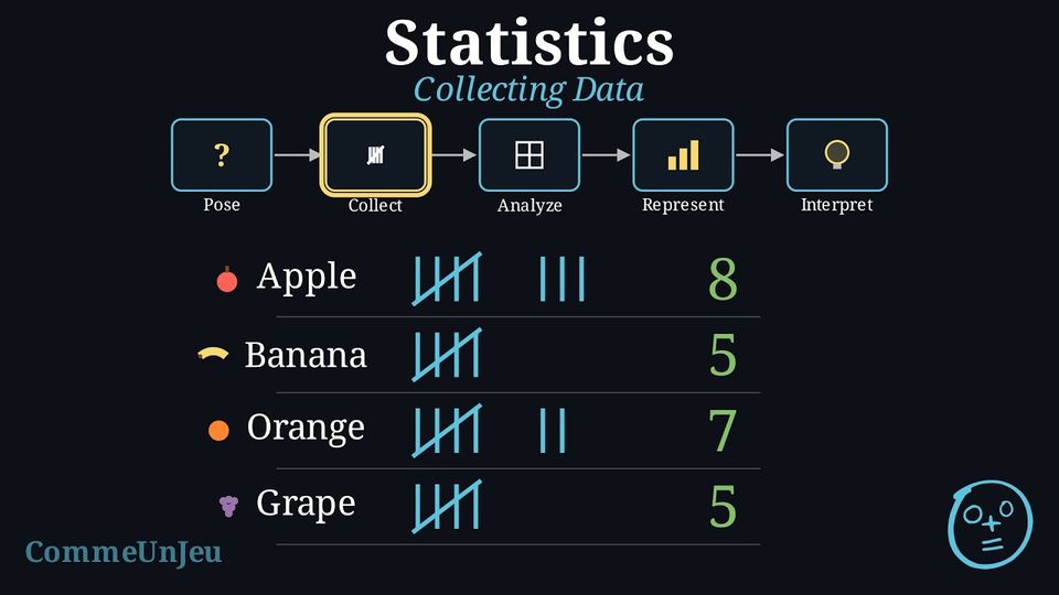
Definition — Population
A population is the entire group of people or things to be studied.
When we conduct an investigation, we must decide who to collect data from. Do we ask everyone in the population, or just a smaller group?
Definition — Census vs. Survey
- A census collects data from every single member of the population. It gives the exact answer for the population, if everyone answers, but it can be very slow and expensive for large populations.
- A survey collects data from a smaller, manageable group taken from the population, called a sample (choosing this group is called sampling). It is much faster, but the sample must be chosen carefully to be representative of the whole population. The word survey also names the questionnaire itself, the list of questions asked.
Example
An investigation asks: “What is the favourite subject of students at this school?”If every student in the school is asked, is it a census or a survey?
It is a census because data are collected from the entire population (all students in the school).
Example
An investigation asks: “What is the favourite subject of students at this school?”If only the students of one Maths class are asked, is it a census or a survey?
It is a survey because data are only collected from a small sample (one Maths class) of the total population (the whole school).
Skills to practice
- Choosing the Correct Data Collection Method
I.2
Representative Samples and Bias
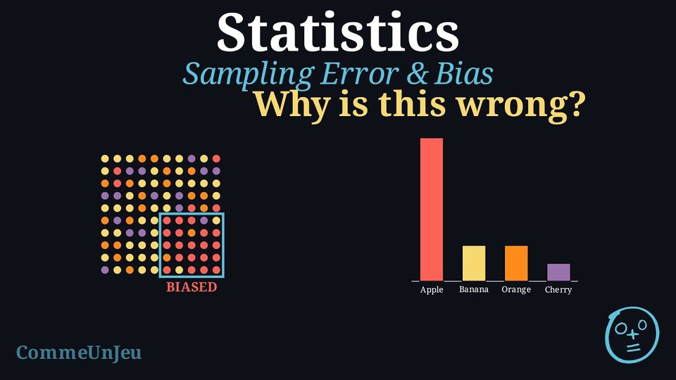
A census asks everyone, but it is often too slow or too expensive. Most investigations therefore use a survey: they study a sample and use it to draw a conclusion about the whole population. For this to work, the sample must give a fair picture of the population. The way the sample is chosen decides whether the conclusion can be trusted.
Definition — Representative Sample
A sample is representative when it reflects the whole population: the different groups inside the population appear in the sample in about the same proportions as in the population. A conclusion drawn from a representative sample can reasonably be extended to the whole population. A sample that is biased leans towards one type of answer and does not reflect the population, so its conclusion cannot be trusted. Definition — Common Sources of Bias
Three ways of building a sample often make it biased: - Convenience: choosing the people who are easiest to reach. Example: to learn the favourite sport of a town, only the people leaving a swimming pool are asked — swimmers are over-represented.
- Voluntary response: letting people decide for themselves whether to answer. Example: a magazine prints a survey and only the readers who feel strongly send it back.
- Undercoverage: leaving part of the population out of the sample completely. Example: to survey a whole school, only the students who own a smartphone are asked — those without one are never reached.
Sample size. A larger sample is generally more reliable, because it captures more of the variety in the population and the result is less likely to change just by chance. However, a bigger sample does not repair a biased method. If the way of choosing people already leans in one direction, asking more of the same kind of people only makes the biased result look more convincing without making it more correct. A small fair sample is worth more than a large biased one: it is less precise, but it is not biased.
Example
A school wants to know the favourite breakfast of all its students. To save time, a survey is carried out by asking the first 60 students arriving at the door of the canteen one morning. State whether this sample is representative. If it is biased, name the source of bias.
The sample is biased, so it is not representative of the whole school.
- The population is all the students of the school.
- The sample is only the students who go to the canteen, and only those who arrive early.
Skills to practice
- Identifying Representative and Biased Samples
- Explaining and Correcting a Biased Sample
II
Analysing Data
II.1
Measuring the Centre
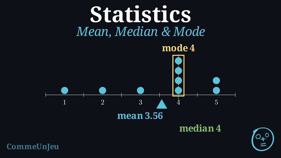
Definition — Measures of Central Tendency
A measure of central tendency is a single value that attempts to describe a set of data by identifying the central position within that set. The main measures are the mean, median, and mode (the mode can also be used for categorical data). Definition — Median
The median is the middle value of a dataset that has been ordered from least to greatest. - If there is an odd number of values, the median is the single middle value.
- If there is an even number of values, there are two middle values and the median is the mean of these two values.
Skills to practice
- Calculating the Median
II.2
Measuring the Spread
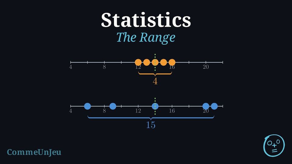
Definition — Measures of Spread (Dispersion)
A measure of spread (or dispersion) describes how varied or “spread out” the values in a dataset are. While a measure of central tendency tells us about the centre, the spread tells us about the consistency of the data, giving a more complete picture than central tendency alone. Definition — Range
The range is the difference between the maximum and minimum values in a dataset. It gives a quick measure of the total spread. $$ \text{Range} = \text{Maximum Value} - \text{Minimum Value} $$ Example
Consider the test scores of two students: - Student A's scores: 10, 50, 90
- Student B's scores: 45, 50, 55
Skills to practice
- Reading the Range on a Bar Chart
II.3
Extreme Values
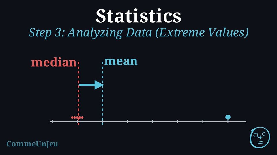
In a small company, the five technicians earn \(\dollar 1\,600\), \(\dollar 1\,800\), \(\dollar 2\,000\), \(\dollar 2\,200\) and \(\dollar 2\,400\) a month. The boss pays himself \(\dollar 14\,000\). A job advert then claims: “in our company, the mean salary is \(\dollar 4\,000\)”. 
Is the advert lying? What does the median salary say?
The advert does not lie: \(\dfrac{1\,600+1\,800+2\,000+2\,200+2\,400+14\,000}{6} = \dfrac{24\,000}{6} = 4\,000\). Yet nobody in the company earns anything close to \(\dollar 4\,000\): the single extreme salary pulls the mean up. The median salary — \(\dfrac{2\,000+2\,200}{2} = 2\,100\) — describes the typical pay much better — that is the whole point of choosing between mean and median. 
Proposition — Effect of an Extreme Value
An extreme value (much larger or much smaller than the others) pulls the mean towards it, because the mean uses all the values. Adding or removing one value shifts the median by at most one position in the ordered list: it moves at most to a neighbouring value — for tightly grouped data, little or not at all.When a dataset contains an extreme value, the median often describes the typical value better than the mean does.
Example
The marks of five friends at a test are \(9\), \(10\), \(11\), \(12\), \(13\). - Compute the mean and the median of these five marks.
- A sixth friend, absent that day, hands in a blank paper: a mark of \(0\) joins the dataset. Compute the new mean and the new median.
- Which measure changed the most?
- Mean: \(\dfrac{9+10+11+12+13}{5} = \dfrac{55}{5} = \textcolor{colorprop}{11}\). The ordered list has \(5\) values, the middle one is the third: median \(= \textcolor{colorprop}{11}\).
- New dataset, ordered: \(0, 9, 10, 11, 12, 13\). Mean: \(\dfrac{55+0}{6} = \dfrac{55}{6} \approx \textcolor{colorprop}{9.2}\). With \(6\) values, the median is the mean of the third and fourth: \(\dfrac{10+11}{2} = \textcolor{colorprop}{10.5}\).
- The mean dropped by almost \(2\) points; the median only by \(0.5\). The extreme value \(0\) pulled the mean, while the median resisted.

Skills to practice
- Recognising the Effect of an Extreme Value
- Choosing Between the Mean and the Median
- Judging the Mean and Choosing a Summary
II.4
Comparing Two Data Sets
Method — Comparing Two Data Sets
- Compare a measure of centre: the means — or the medians if one dataset contains an extreme value.
- Compare a measure of spread: the ranges — or another measure of spread already known.
- Conclude in the context: the same centre with different spreads means “same typical level, but not the same regularity”.
Example
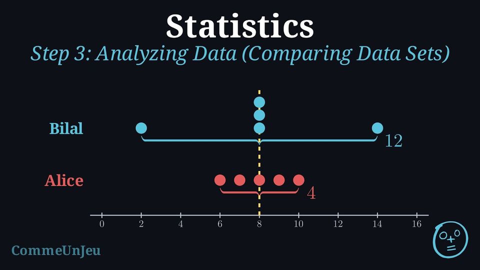
Alice and Bilal each shot five rounds at the archery club. | Alice | 6 | 7 | 8 | 9 | 10 |
| Bilal | 2 | 8 | 8 | 8 | 14 |
Position: Alice \(\dfrac{6+7+8+9+10}{5} = \dfrac{40}{5} = \textcolor{colorprop}{8}\); Bilal \(\dfrac{2+8+8+8+14}{5} = \dfrac{40}{5} = \textcolor{colorprop}{8}\) — and both medians are \(8\) too. The two archers have the same typical level.
Spread: Alice \(10-6 = \textcolor{colorprop}{4}\); Bilal \(14-2 = \textcolor{colorprop}{12}\).
In context: same level, but Alice's range is three times smaller — she is the more regular of the two; Bilal can shoot a \(14\) — and a \(2\). 
Spread: Alice \(10-6 = \textcolor{colorprop}{4}\); Bilal \(14-2 = \textcolor{colorprop}{12}\).
In context: same level, but Alice's range is three times smaller — she is the more regular of the two; Bilal can shoot a \(14\) — and a \(2\).
Skills to practice
- Comparing Two Data Sets
III
Representing Data
III.1
Choosing a Suitable Representation
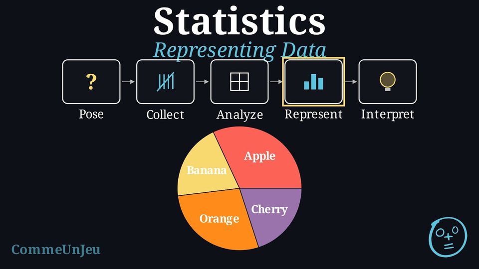
Once data is organised in a table, we can create graphs to see the patterns visually. Bar charts are excellent for comparing the numbers of answers (the frequencies), while pie charts are best for showing proportions.
Skills to practice
- Choosing a Suitable Representation
III.2
Spotting a Misleading Graph
A graph is meant to show data honestly, but the same numbers can be drawn in ways that push the reader toward a wrong impression. The data may be exact while the picture exaggerates or hides a difference. Recognising these tricks is part of reading data critically.
Method — How a Graph Can Mislead
Three common ways make a graph misleading: - Truncated axis: the vertical axis of a bar chart does not start at 0. A small difference in the values then looks like a huge difference, because the eye compares the heights drawn, not the true numbers.
- Distorted scale: the intervals on an axis are not equal (for example \(0, 10, 20, 50, 100\) spaced evenly). Equal steps on the paper no longer mean equal steps in the data, so the shape of the graph is deformed.
- Area or 3-D distortion: making a picture, an icon, or a slice “bigger” by enlarging its width and height (or adding depth) multiplies the area, which exaggerates a difference that is really small.
Example
Two shops belong to the same chain. Last month, Shop A made 52 sales and Shop B made 48 sales. The two bar charts below show exactly these numbers. The chart on the left uses a vertical axis starting at 45; the chart on the right uses a vertical axis starting at 0. Explain why the left chart is misleading and which chart should be used. 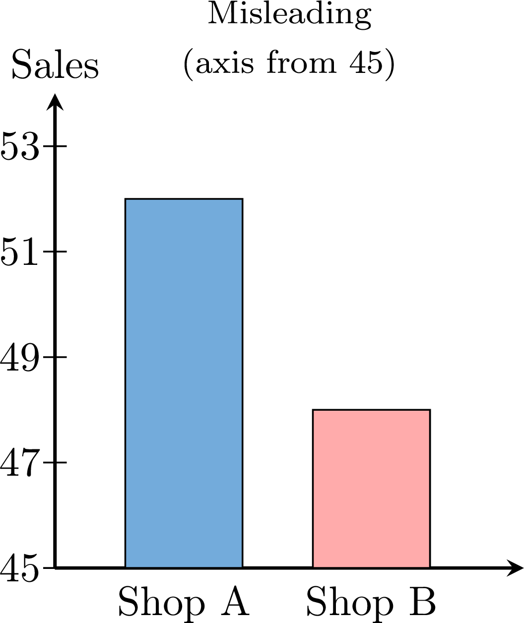 \(\qquad\quad\)
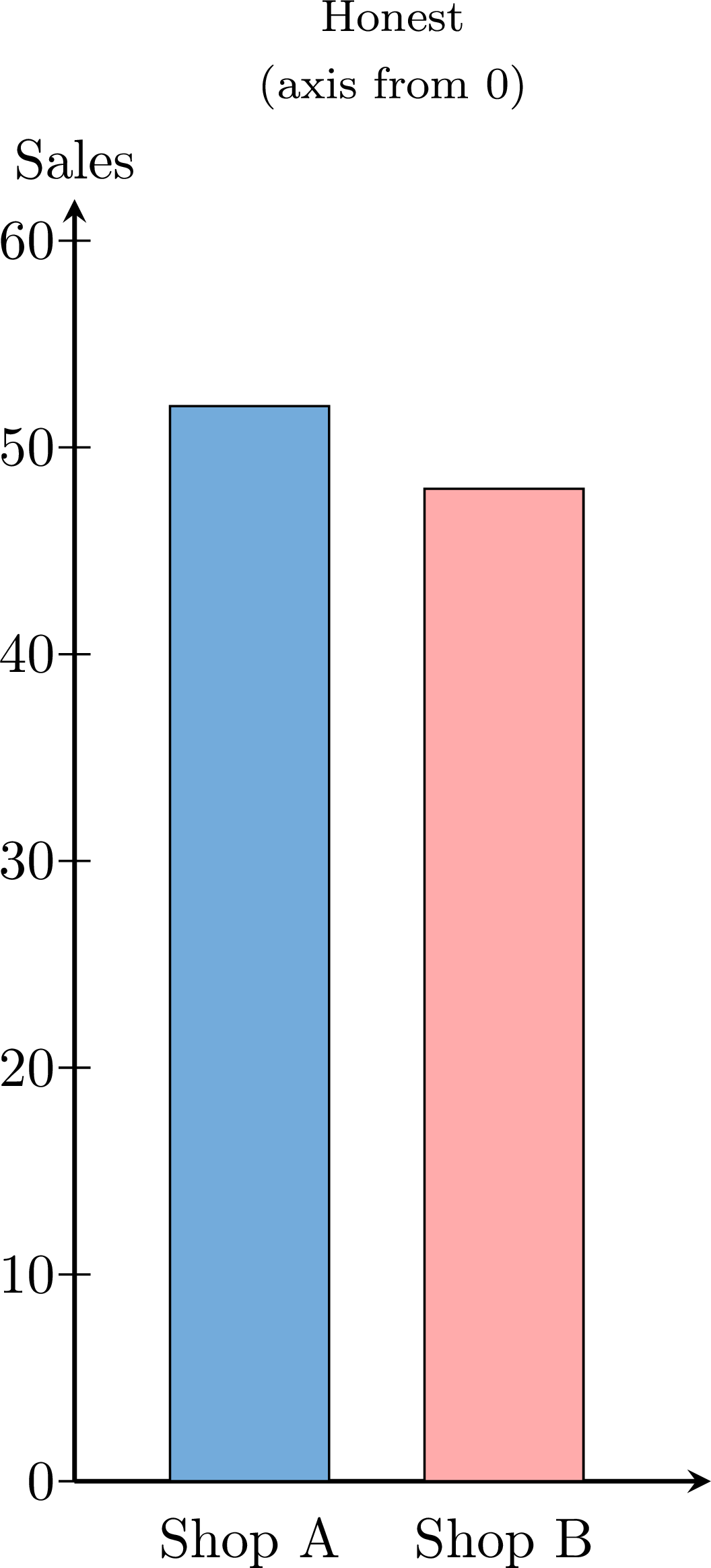
Both charts show the same true data: 52 sales for Shop A and 48 for Shop B, a difference of only 4 sales. In the left chart the vertical axis starts at 45 instead of 0 (a truncated axis), so only the top of each bar is drawn. The bar for Shop A then reaches a height of \(52-45=7\) units while the bar for Shop B reaches \(48-45=3\) units. On paper, Shop A's bar looks more than twice as tall as Shop B's, suggesting Shop A sold far more — yet \(52\) is only about \(8\pourcent\) more than \(48\). The right chart starts the axis at 0, so the bar heights are proportional to the real numbers and the two shops correctly appear almost equal. The honest chart (axis from 0) is the one that should be used.
Method — Reading a Graph Critically
Before trusting what a graph seems to show, run these checks: - Check the vertical axis of a bar chart starts at 0: if it starts higher, small differences are being exaggerated.
- Check the scale is regular: the intervals on each axis should be equal, so equal distances mean equal amounts.
- Beware of pictures and 3-D: an image or slice made “bigger” in two directions, or drawn in 3-D, can exaggerate a small difference through its area.
- Go back to the numbers: when in doubt, read the actual values and compare them directly rather than trusting the drawn heights.
Skills to practice
- Detecting Misleading Graphs
III.3
Drawing and Reading Stem-and-Leaf Plots
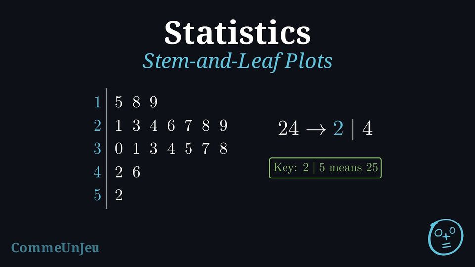
A list of numbers is hard to read, and when most values are different, a bar chart with one bar for each value would have almost as many bars as there are values. A stem-and-leaf plot sorts the values into rows, like a bar chart turned on its side, and still shows every value.
Definition — Stem-and-Leaf Plot
A stem-and-leaf plot (or stemplot) displays numerical data by splitting each value into a stem, made of all its digits except the last one, and a leaf, its last digit; a one-digit value such as \(8\) has the stem \(0\). - The stems are written once each, in increasing order, in a column to the left of a vertical line.
- Each value writes its leaf in the row of its stem, the leaves being evenly spaced.
- In an ordered stem-and-leaf plot, the leaves of each row are in increasing order.
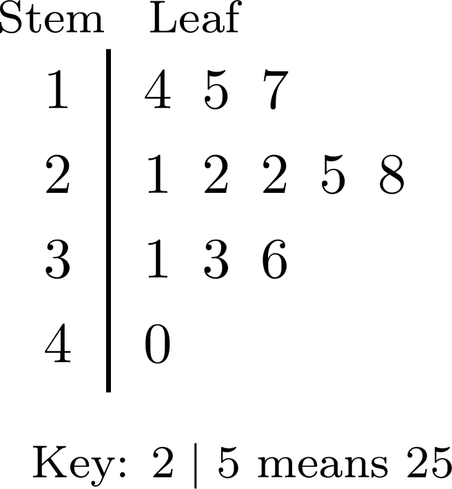
- A key, such as “\(2 \mid 5\) means \(25\)”, gives the place value of the leaves. For decimals, the key gives the place value of the leaf: with the key “\(2 \mid 4\) means \(0.24\)”, the stem is the tenths digit and the leaf the hundredths digit.
Method — Drawing an Ordered Stem-and-Leaf Plot
- Find the smallest and the largest values, and choose the stems that cover them: for values from \(15\) to \(52\), the stems are \(1\), \(2\), \(3\), \(4\), \(5\).
- Write the stems in a column, in increasing order, with no stem missing between the first and the last, and draw a vertical line to their right.
- Go through the list once, in its order, writing the leaf of each value in the row of its stem, and crossing out the value in the list.
- Order each row: write the plot again with the leaves of each row in increasing order, evenly spaced, so that the rows can be compared like bars.
- Add a key and a title, and check that the number of leaves equals the number of values.
Example
The times, in minutes, that \(20\) pupils spent on their homework one evening are: $$\begin{aligned}&24,\ 35,\ 18,\ 42,\ 31,\ 27,\ 15,\ 38,\ 29,\ 33,\\
&21,\ 46,\ 30,\ 26,\ 19,\ 37,\ 28,\ 52,\ 34,\ 23.\end{aligned}$$ Draw an ordered stem-and-leaf plot of these times.
The smallest time is \(15\) and the largest is \(52\): the stems are the tens digits \(1\) to \(5\). Going through the list in its order gives the plot on the left; ordering each row gives the plot on the right. 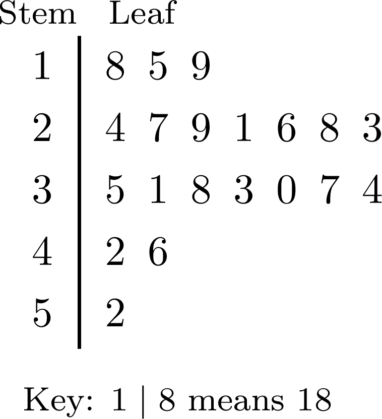 \(\qquad\)
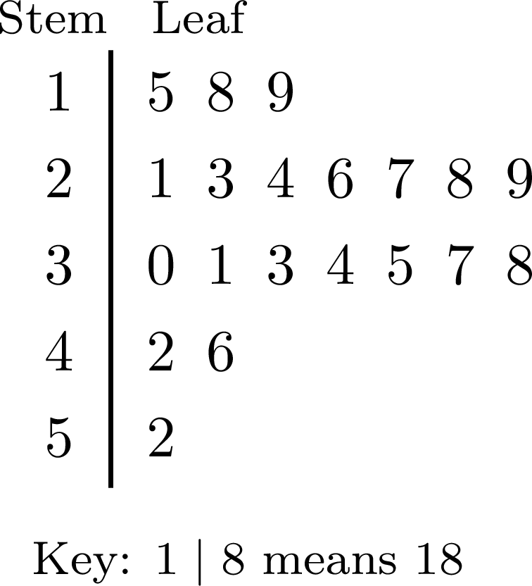
The plot has \(3 + 7 + 7 + 2 + 1 = 20\) leaves, one for each pupil. Most pupils spent between \(20\) and \(39\) minutes, and the time of \(52\) minutes stands a little apart.
\(\qquad\) Example
The masses of the school bags of \(15\) pupils were weighed to the nearest \(0.1\) kg. 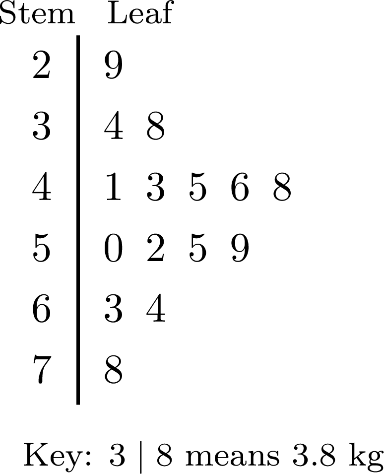
- Find the mass of the lightest bag and of the heaviest bag.
- How many bags weigh at least \(5\) kg?
- What percentage of the bags weigh more than \(6\) kg?
- Which row holds the most bags? Which value stands apart from the others?
The key says that the stem is the whole number of kilograms and the leaf the tenths: \(3 \mid 8\) is \(3.8\) kg.
- The first leaf of the first row gives the lightest bag, \(2.9\) kg; the last leaf of the last row gives the heaviest, \(7.8\) kg.
- The bags of at least \(5\) kg are those of the rows \(5\), \(6\) and \(7\): \(4 + 2 + 1 = 7\) bags.
- The bags of more than \(6\) kg are \(6.3\), \(6.4\) and \(7.8\) kg, that is \(3\) bags out of \(15\): $$\frac{3}{15} \times 100\pourcent = 20\pourcent.$$
- The row \(4\) holds \(5\) bags, the most: bags from \(4.0\) to \(4.9\) kg are the most common. The value \(7.8\) kg stands apart: the row \(7\) has only this leaf, and it is far from the others.
Why a Stem-and-Leaf Plot Needs a Key
Without its key, the row \(3 \mid 4\ 8\) can stand for \(34\) and \(38\), for \(3.4\) and \(3.8\), or for \(0.34\) and \(0.38\): only the key says which place value the leaves have. A stem-and-leaf plot keeps every value, while a bar chart only shows how many values fall in each category. It suits sets of a few dozen values; with hundreds of values, the rows become too long to read.
Example
The ordered stem-and-leaf plot gives the numbers of push-ups that the \(21\) pupils of a class did in one minute. 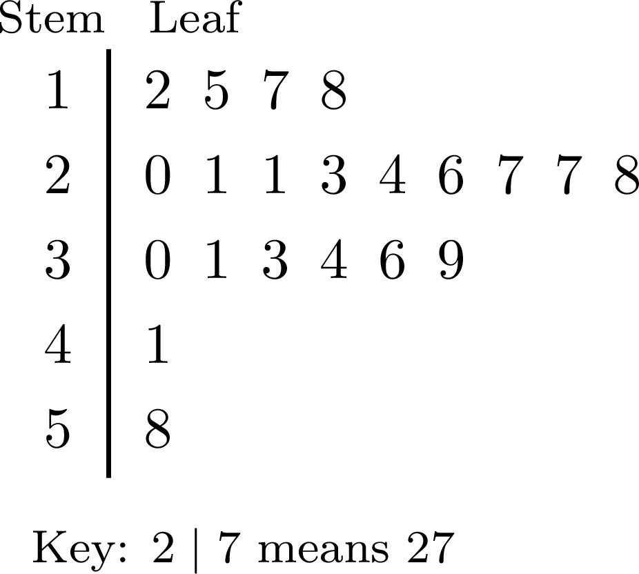
- Find the median and the range of these numbers.
- The value \(58\) is an extreme value. Find the median and the range of the \(20\) other values.
An ordered stem-and-leaf plot lists the values in increasing order: the median and the range are read without writing the list again.
- There are \(21\) values, an odd number: the median is the \(11^{\text{th}}\) value. The row \(1\) holds the \(1^{\text{st}}\) to the \(4^{\text{th}}\) values; counting on in the row \(2\), the \(5^{\text{th}}\) to the \(11^{\text{th}}\) values are \(20\), \(21\), \(21\), \(23\), \(24\), \(26\), \(27\). The median is \(27\) push-ups.
The smallest value is the first leaf, \(12\), and the largest the last leaf, \(58\): $$\begin{aligned}[t] \text{range} &= \text{maximum} - \text{minimum} && \text{(definition of the range)}\\ &= 58 - 12\\ &= 46 \text{ push-ups}. \end{aligned}$$ - Without \(58\), there are \(20\) values: the median is the mean of the \(10^{\text{th}}\) and \(11^{\text{th}}\) values, \(\dfrac{26 + 27}{2} = 26.5\) push-ups, and the range is \(41 - 12 = 29\) push-ups. The extreme value made the range much larger, from \(29\) to \(46\), while the median only moved by half a place, as the Proposition “Effect of an Extreme Value” says.
Outliers
An extreme value that lies unusually far from the rest of a data set is also called an outlier. On a dot plot, or in an ordered stem-and-leaf plot, an outlier stands apart from the rest of the data. The ordered stem-and-leaf plot below shows the times, in minutes, that \(14\) runners took to finish a cross-country race: the time \(69\) min is separated from the others by an empty row. 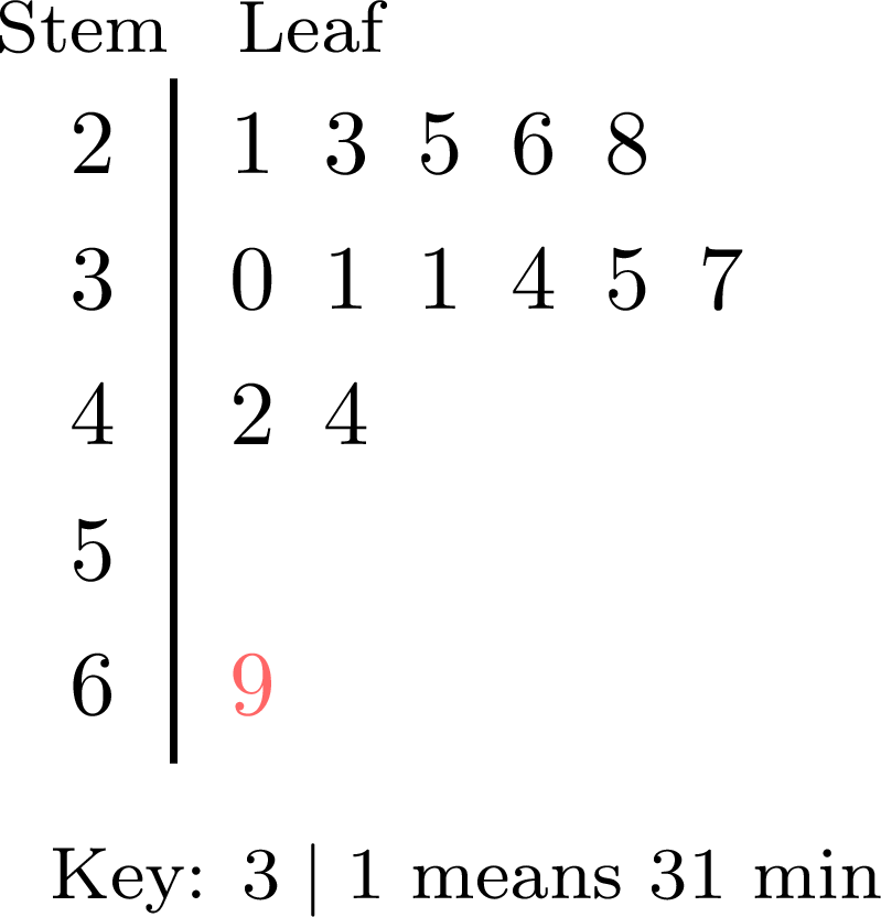
Before using an outlier, check where it comes from.
- If it is a mistake, such as a typing error or a value written in the wrong unit, it is corrected, or removed from the data.
- If it is a genuine value, such as a runner who fell and walked to the finish, it is usually kept, unless the question is only about the other cases. It pulls the mean towards it and stretches the range, while it moves the median by at most one position in the ordered list: the median then often describes the typical value better.
Skills to practice
- Checking a Reading of a Stem-and-Leaf Plot
- Reading Stem-and-Leaf Plots
- Drawing Stem-and-Leaf Plots
III.4
Horizontal Bar Charts and Side-by-Side Column Graphs
Definition — Horizontal Bar Chart
In a horizontal bar chart, the categories are written along the vertical axis and the bars are drawn horizontally: the length of each bar, read on the horizontal axis, gives the frequency of its category. It is convenient when the names of the categories are long. The chart below shows the favourite subjects of \(25\) pupils. 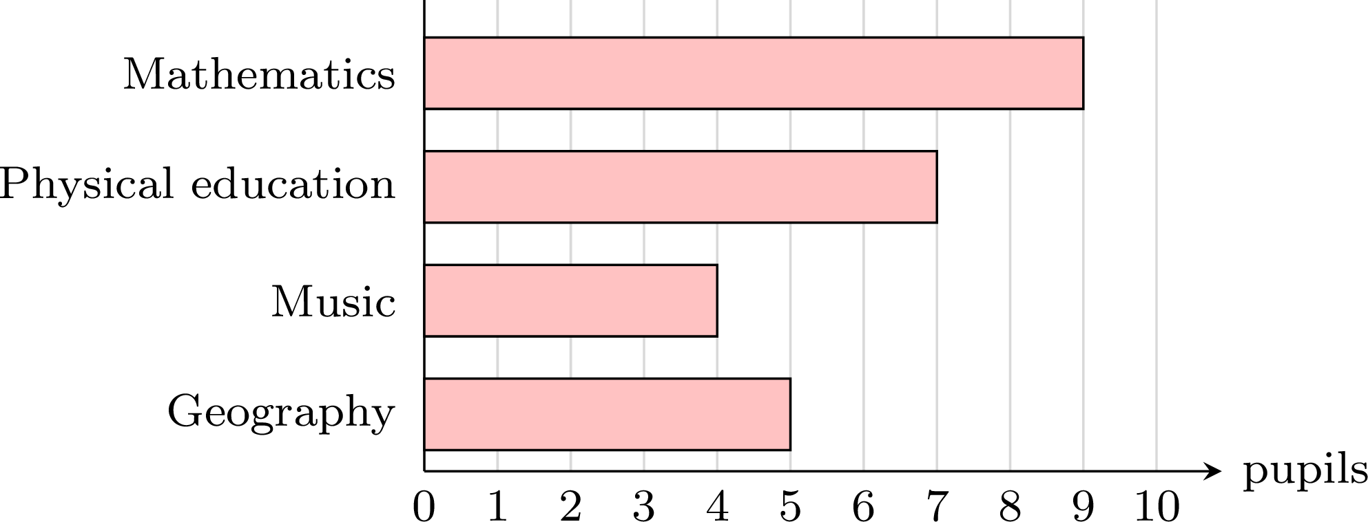
Definition — Side-by-Side Column Graph
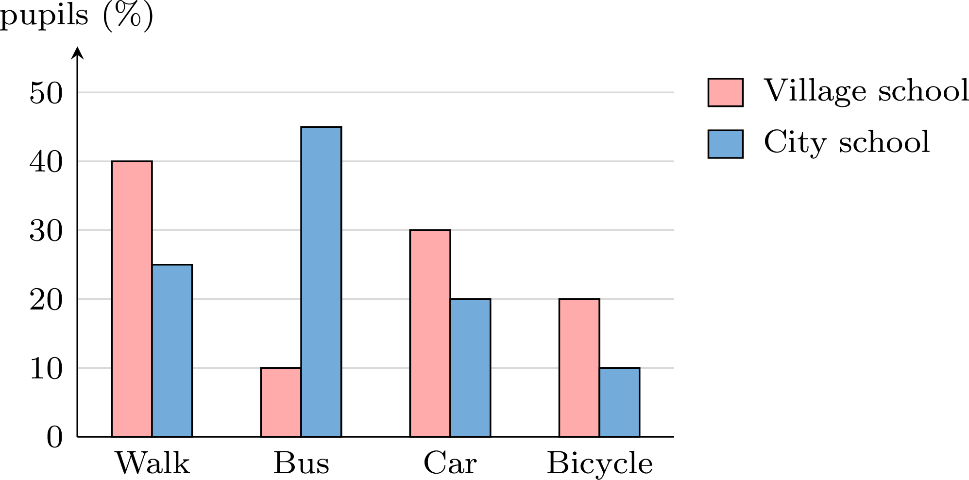
A side-by-side column graph (or compound bar chart) compares two or more groups over the same categories: for each category, one column per group is drawn, the columns of the category standing side by side. Each group has its own colour, explained by a legend. The graph below compares the snacks sold by a school canteen on Monday and on Tuesday. 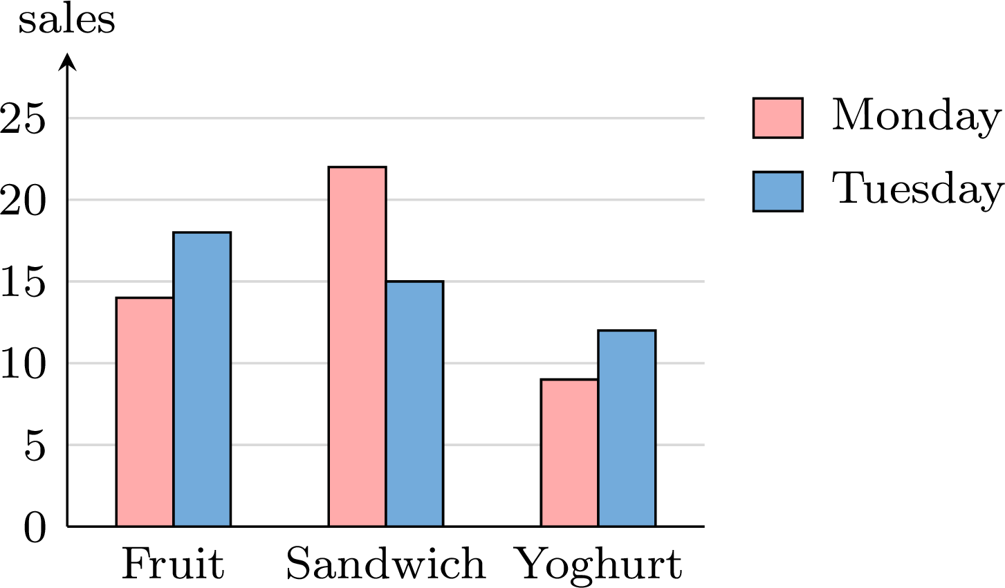
Example
The \(25\) pupils of class A and the \(25\) pupils of class B named their favourite sport. | Sport | Football | Basketball | Swimming | Tennis | Other |
| Class A | \(8\) | \(5\) | \(6\) | \(4\) | \(2\) |
| Class B | \(5\) | \(7\) | \(4\) | \(3\) | \(6\) |
For each sport, the column of class A and the column of class B stand side by side, on the same vertical scale starting at \(0\). 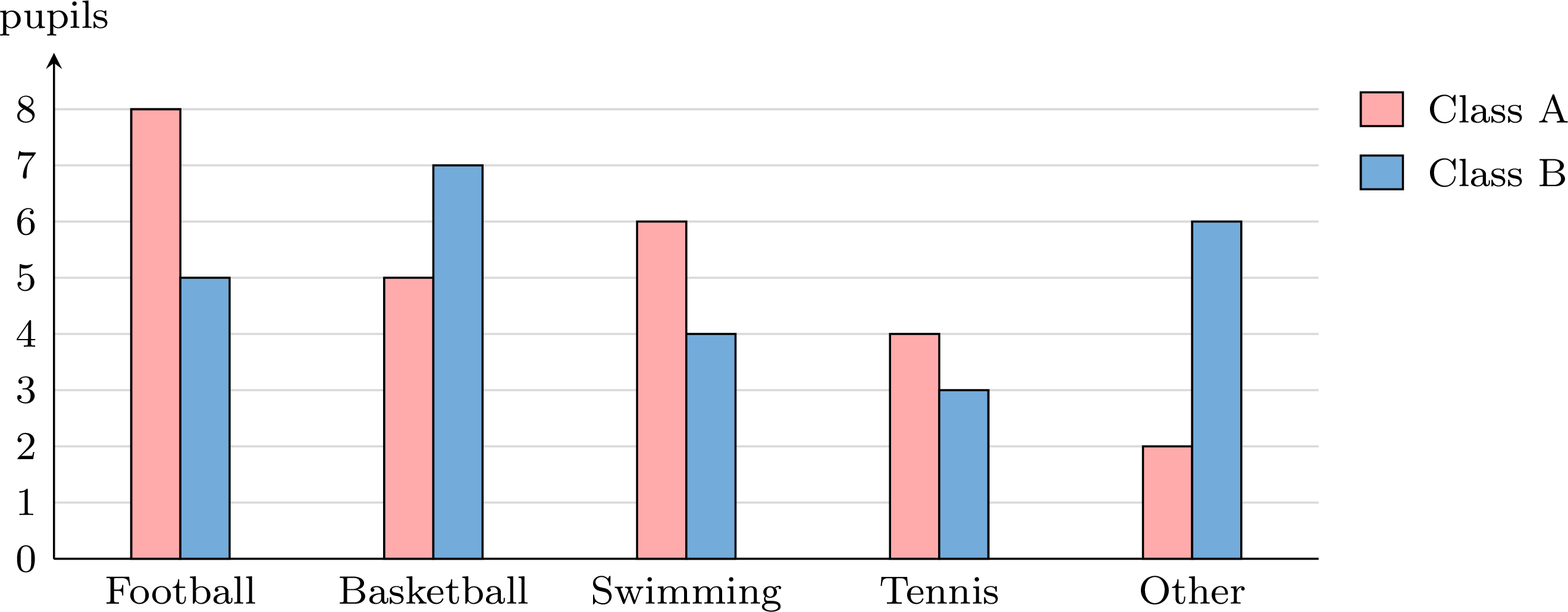
The two classes have the same size, \(25\) pupils, so their columns can be compared directly. Football is the favourite sport of class A (\(8\) pupils) and basketball that of class B (\(7\) pupils). Class A prefers swimming more than class B does (\(6\) against \(4\)), while “other” sports are much more frequent in class B (\(6\) against \(2\)).
Comparing Groups of Different Sizes
When the groups do not have the same size, their frequencies answer the question “in which group are there more?”, not the question “in which group is it more common?”: \(10\) pupils out of \(40\) are more pupils, but a smaller share, than \(8\) pupils out of \(20\). To compare the shares, the side-by-side column graph is drawn with the relative frequencies of each group, written as percentages, so that every group counts out of \(100\).
Example
The pupils of a village school and of a city school said how they come to school. | Walk | Bus | Car | Bicycle | Total | |
| Village school | \(8\) | \(2\) | \(6\) | \(4\) | \(20\) |
| City school | \(10\) | \(18\) | \(8\) | \(4\) | \(40\) |
- In which school do more pupils walk to school? In which school is walking more common?
- Draw a side-by-side column graph that compares the two schools fairly.
- More pupils walk at the city school: \(10\) against \(8\). But the city school has twice as many pupils, so the shares must be compared: $$\frac{8}{20} \times 100\pourcent = 40\pourcent \qquad \text{and} \qquad \frac{10}{40} \times 100\pourcent = 25\pourcent.$$ Walking is more common at the village school.
- In the same way, the village school gives \(\frac{2}{20} = 10\pourcent\) by bus, \(30\pourcent\) by car and \(20\pourcent\) by bicycle; the city school gives \(\frac{18}{40} = 45\pourcent\) by bus, \(20\pourcent\) by car and \(10\pourcent\) by bicycle. The graph shows these percentages.
Skills to practice
- Checking a Reading of a Bar Chart
- Reading Bar Charts and Side-by-Side Column Graphs
- Drawing and Comparing Bar Charts
III.5
Infographics
Definition — Infographic
An infographic presents data as a picture designed to be read at a glance, in a newspaper, on a poster or on a website. It usually combines: - a headline, which states the message;
- a few key numbers, printed large;
- icons or pictograms, and one or two simple charts;
- the source of the data: who collected them, when, and from how many people.
Method — Reading an Infographic Critically
Before trusting an infographic, answer six questions. - Where do the data come from? Read the source: who collected the data, when, and how many people were asked. A sample chosen among the people most concerned is likely to be biased when the results are meant to describe a wider population. A very small sample describes only the people asked: as a guide to a whole population it is unreliable, since another small sample could give a very different result.
- What is counted, out of what total? A percentage is always a percentage of a total. The percentages given for one question add up to \(100\pourcent\), up to rounding, when each person gave exactly one answer and every answer is shown. If they add up to clearly more, beyond rounding, either several answers were allowed or there is a mistake: the infographic should say which. If they add up to less, something is missing: a category, or the people who did not answer — unless the gap is only due to rounding.
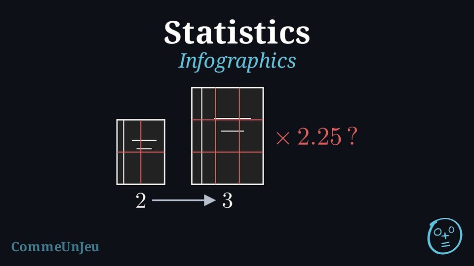
- Do the pictures match the numbers? An icon enlarged in height and in width grows in area much faster than the number it stands for: it is the area trap of a misleading graph. An honest infographic repeats icons of the same size, each worth the same amount, and gives a key.
- Is the comparison fair? Counts say how many; to compare groups of different sizes, compare percentages. Two periods can be compared only if the data were collected in the same way, and two numbers only if they have the same unit.
- Can a number be checked? Recompute a total or a percentage from the other numbers.
- What does it show, and what does it not show? Conclude with one sentence for each, naming the people who were really asked.
Example
The infographic below was published on a website for teenagers. 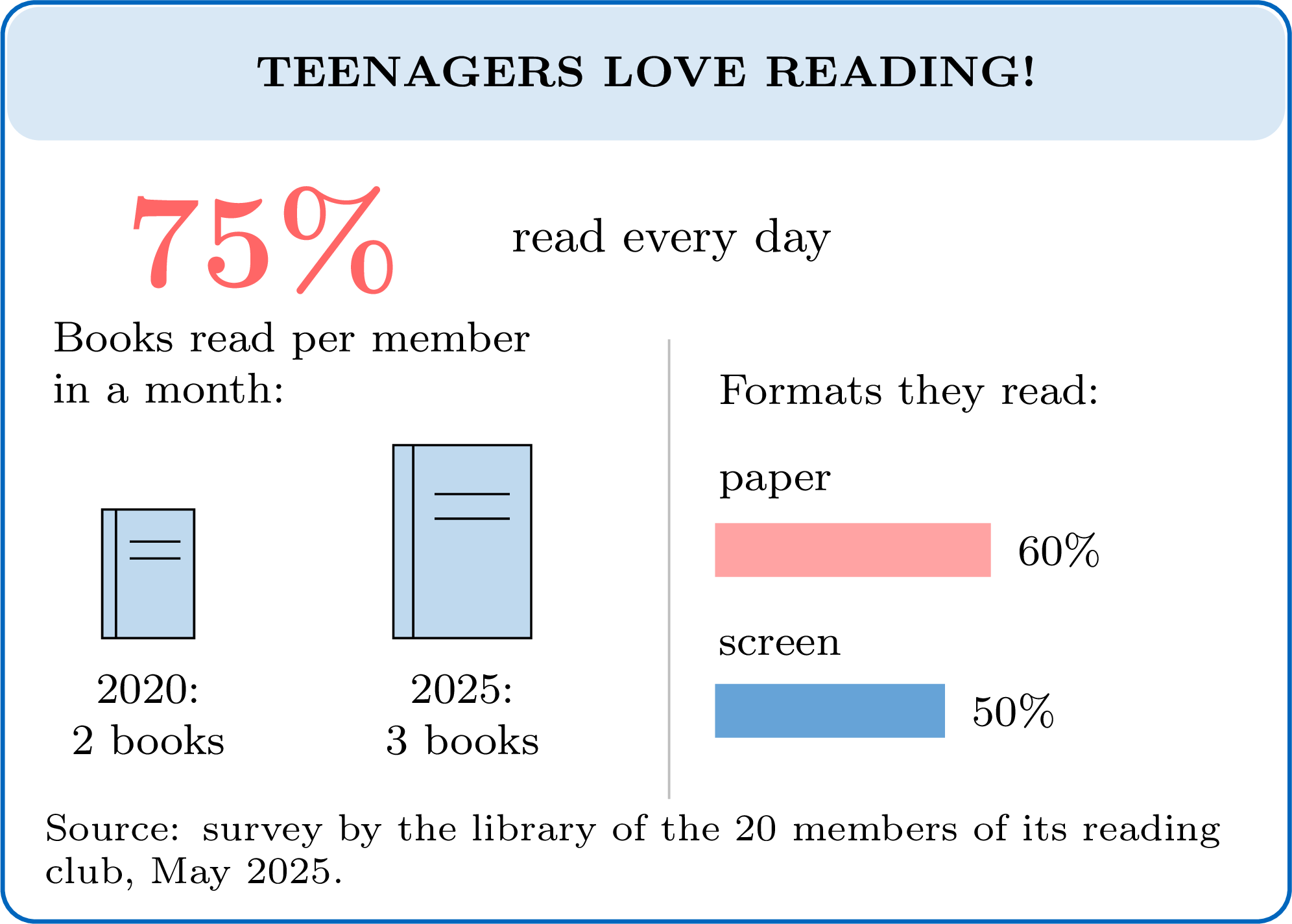
- Source. Only \(20\) people were asked, all members of a reading club. The sample is small, and it is probably biased: people who join a reading club are likely to read more than most teenagers. Yet the headline speaks about all teenagers.
- What is counted. \(75\pourcent\) of the \(20\) members is \(15\) members. The two formats give \(60\pourcent + 50\pourcent = 110\pourcent\), more than \(100\pourcent\). Members may read both formats, so several answers were probably allowed; if only one answer had been allowed, the numbers would contain a mistake. The infographic should say which, and in both cases the two bars are not two parts of one whole.
- Pictures. From \(2\) books to \(3\) books, the number is multiplied by \(\dfrac{3}{2} = 1.5\). But the second book is drawn \(1.5\) times taller and \(1.5\) times wider, so its area is \(1.5 \times 1.5 = 2.25\) times larger: the picture suggests that reading has more than doubled. An honest version draws \(2\) books, then \(3\) books, all of the same size.
- Fair comparison. The source describes only the survey of May 2025: nothing says who was asked in 2020, so the two years may not be comparable.
- Check. \(75\pourcent\) of \(20\) gives \(15\), a whole number of members, as it must. \(60\pourcent\) of \(20\) is \(12\) and \(50\pourcent\) of \(20\) is \(10\): \(12 + 10 = 22\) answers from \(20\) members, so, if several answers were allowed, at least \(22 - 20 = 2\) members chose both formats.
- Conclusion. The infographic shows that \(15\) of the \(20\) members of one reading club said, in May 2025, that they read every day. It does not show that teenagers in general read every day, nor that reading grew as much as the picture of the books suggests.
Method — Building a Simple Infographic
- Start from one question, and write a headline that answers it, saying no more than the data show.
- Choose two or three key numbers and compute them from the data: a percentage of the total, the mode, or the mean of numerical data.
- Choose one chart for each message: a pie chart, or a picture split into parts, for the parts of a whole, when the categories do not overlap and together cover everyone; a bar chart to compare categories.
- Draw repeated icons of the same size, each worth the same amount, and give a key; never enlarge an icon.
- Write the source: who was asked, when, and how many people.
- Check every number against the data before publishing.
Example
In September, a class surveyed its \(25\) pupils about how they come to school. | Way of travel | On foot | Bicycle | Bus | Car |
| Pupils | \(10\) | \(5\) | \(8\) | \(2\) |
Key numbers. Each pupil is \(\dfrac{1}{25}\) of the class, that is \(4\pourcent\), so each count is multiplied by \(4\):
Check: \(40 + 20 + 32 + 8 = 100\). On foot or by bicycle: \(10 + 5 = 15\) pupils, and \(\dfrac{15}{25} = \dfrac{3}{5} = 60\pourcent\).
Headline. “3 out of 5 pupils come on foot or by bicycle”: it answers the question and says no more than the data.
Chart and icons. One icon for each pupil, all of the same size, coloured by way of travel: the \(25\) icons show the parts of the whole class at a glance, and the key gives each count and its percentage.
Source. Who collected the data, who was asked, how many, and when. 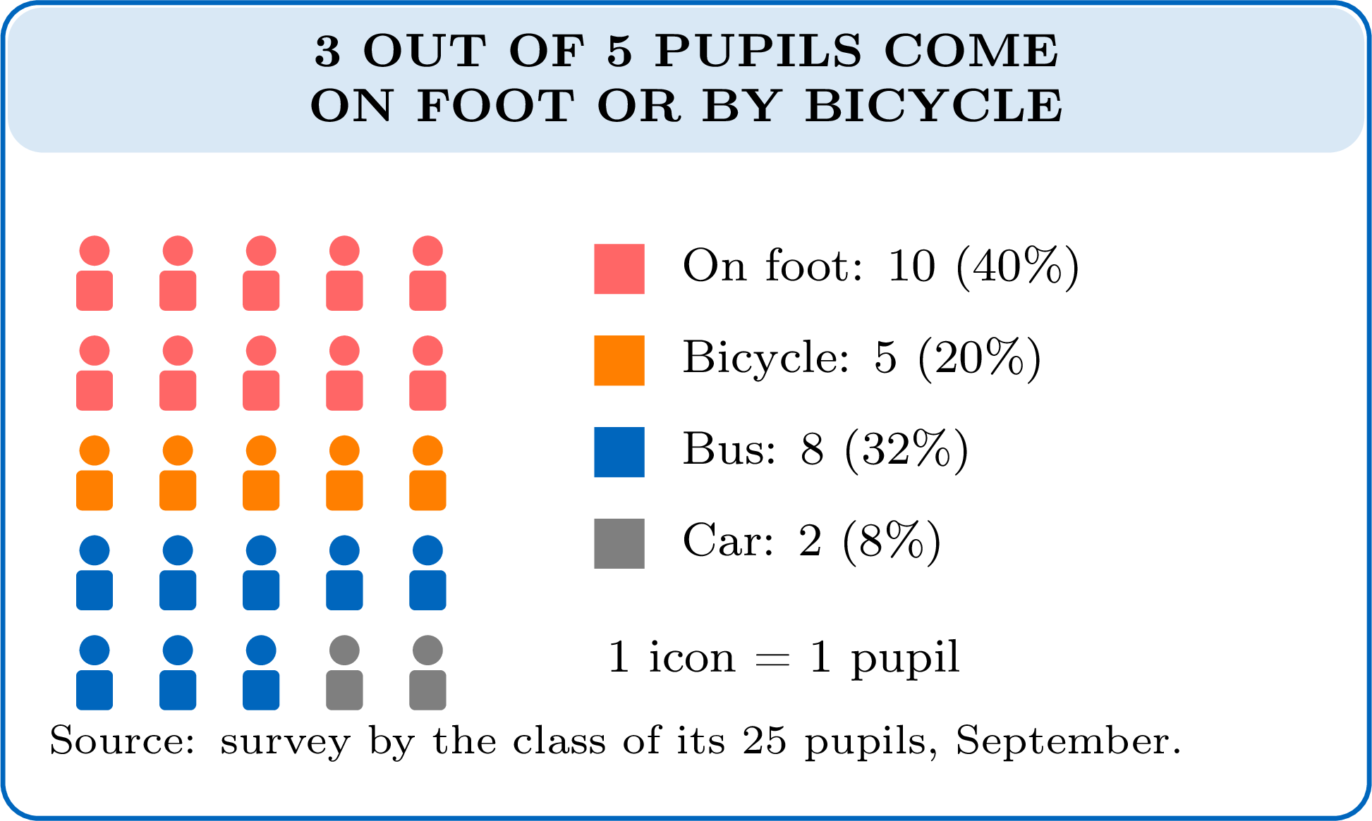
| Way of travel | On foot | Bicycle | Bus | Car |
| Pupils | \(10\) | \(5\) | \(8\) | \(2\) |
| Percentage | \(40\pourcent\) | \(20\pourcent\) | \(32\pourcent\) | \(8\pourcent\) |
Headline. “3 out of 5 pupils come on foot or by bicycle”: it answers the question and says no more than the data.
Chart and icons. One icon for each pupil, all of the same size, coloured by way of travel: the \(25\) icons show the parts of the whole class at a glance, and the key gives each count and its percentage.
Source. Who collected the data, who was asked, how many, and when.
Skills to practice
- Judging an Infographic
- Reading Numbers from an Infographic
- Criticising and Improving Graphs and Infographics
IV
Going further
Skills to practice
- Conducting Investigations and Solving Problems
- Investigating Patterns in Data Summaries
- Quiz
Jump to section