International Baccalaureate · MYP 1
Statistics
I
The Statistical Investigation
I.1
The Five Steps of an Investigation
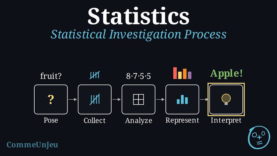
Statistics are all around us, from sports averages to news reports about the weather.
- A basketball player averages 14.6 points per game.
- Last year was the hottest year on record since 1897.
Method — Statistical Investigation Process
A statistical investigation follows these five key steps: - Pose the Question: Define clearly what is to be investigated.
- Collect Data: Gather information relevant to the question.
- Analyse Data: Count, compute proportions, and later on means.
- Represent Data: Display the organised data visually using graphs and charts.
- Interpret Data: Draw conclusions to answer your question.
Skills to practice
- Identifying the Steps of an Investigation
II
Posing the Question and Collecting Data
II.1
The Statistical Question
Definition — Statistical Question
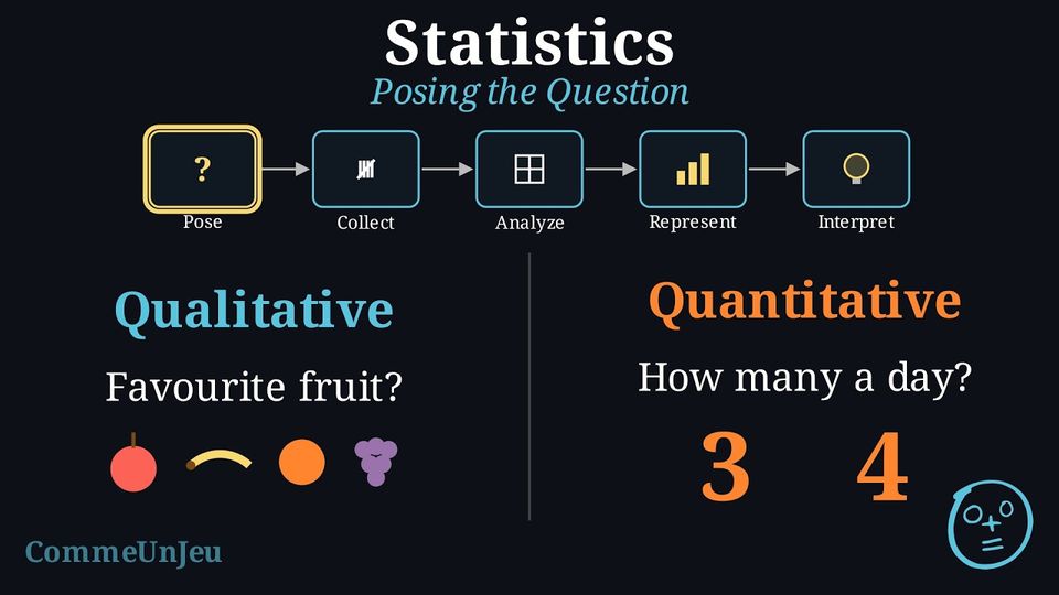
A statistical question is a clear, focused question that is answered by collecting and analysing data, and whose answers vary: from one person or one object to another, the answer is not always the same. Example
We investigate the statistical question: “What is the favourite school subject of the pupils in our class?” The answers vary from one pupil to another. Definition — Qualitative and Quantitative Variables: Counting or Measuring
A survey looks at a variable: what is observed for each person or each object. - a qualitative variable (the answers are categorical data): the answer names a category (eye colour, favourite food), even when it is written with a number, like a shirt number;
- a quantitative variable (the answers are numerical data): the answer says how many. It is counted (the number of siblings) or measured (height in centimetres, mass in kilograms, a duration).
Skills to practice
- Recognising a Statistical Question
II.2
Recording Data with a Tally
Method — Collecting and Recording Survey Data
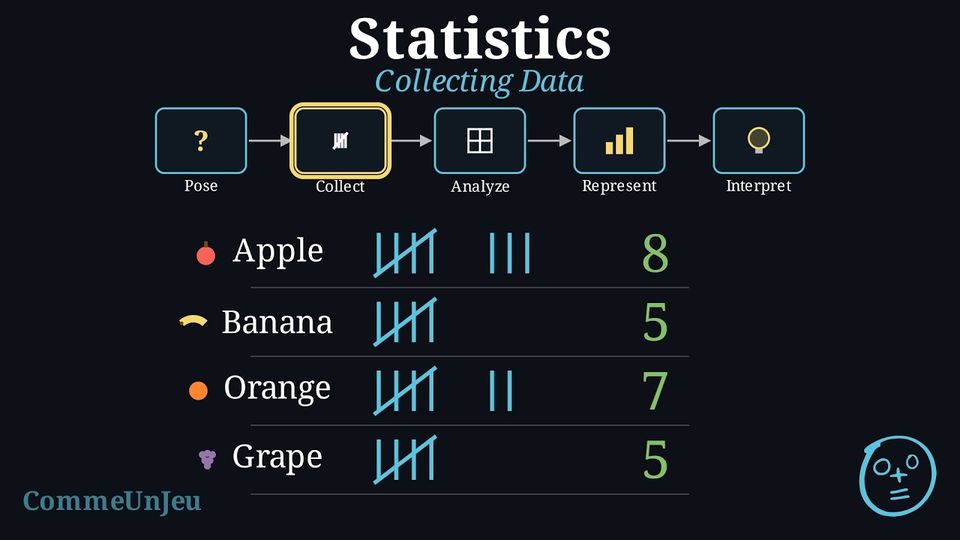
Once the question is posed and the population identified, a systematic way to collect and record the answers is needed. To ask everyone in a small group, such as a class (a census), a tally table is an efficient tool. - Prepare a Tally Table: Before starting, draw a table with a row for each possible answer category and a column for tally marks.
- Conduct the Survey: Ask each person in the population the survey question, one by one.
- Record Each Answer: For each answer received, place one tally mark
 in the row for the corresponding category. The fifth mark is a diagonal line across the first four
 to make counting easier.
Example
Collecting data for the question “What is your favourite school subject?”Each of the 25 students is asked in turn, and the tally column is filled in along the way. After all 25 students have been asked, the tally table looks like this:
| Subject | Tally Marks |
| Maths |  |
| Science |  |
| Sport |  |
| Art | |
Skills to practice
- Tallying Raw Data
III
Analysing Data
III.1
Expressing Relative Frequencies as Percentages
Definition — Frequency and Relative Frequency
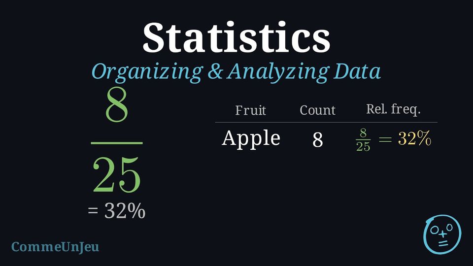
The frequency (or count) of a category is how many times that category appears in our data.Relative frequency is the proportion of the data that falls into a category. We can write it as a fraction, a decimal, or a percentage. $$ \text{Relative frequency (in }\pourcent\text{)} = \frac{\text{Frequency}}{\text{Total number of data values}} \times 100\pourcent $$
Example
We calculate the relative frequency for our “Favourite Subject” survey of 25 students: | Subject | Frequency | Relative Frequency |
| Maths | 8 | \(8/25\times 100\pourcent = 32\pourcent\) |
| Science | 5 | \(5/25\times 100\pourcent = 20\pourcent\) |
| Sport | 7 | \(7/25\times 100\pourcent = 28\pourcent\) |
| Art | 5 | \(5/25\times 100\pourcent = 20\pourcent\) |
| Total | 25 | 100\(\pourcent\) |
Method — Expressing a Proportion as a Percentage from a Table
Once a survey is counted, the table gives a part and a whole. Comparing them answers questions like “is this the majority?” or “is this more than a quarter?”. - Read in the table the number in the category studied: that is the part.
- Add the numbers of the categories (without the totals, if the table has any): that is the whole.
- Write the proportion as a fraction, part over whole.
- Turn it into a percentage: for a whole of \(100\), the numerator is already the percentage; in simple cases (a whole that divides \(100\), or is a multiple of it), look for the equivalent fraction with denominator \(100\).
Skills to practice
- Calculating Relative Frequencies as Percentages
III.2
Summarising Data with the Mode and the Mean
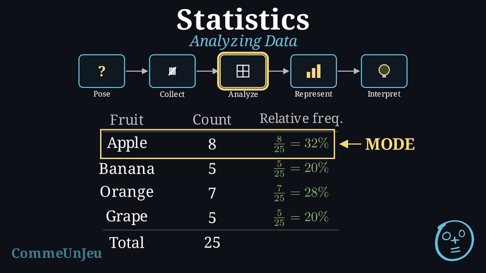
Definition — Mode
The mode is the value or category that appears most frequently. A dataset can have more than one mode. When every value appears the same number of times, the data are said to have no mode. Definition — Mean
The mean is the sum of all numerical values divided by the count of values. It is only used for quantitative data: $$ \bar{x} = \frac{\text{sum of all values}}{\text{number of values}} $$ Example
A survey asked 9 students to rate how much they like their favourite subject on a scale from 0 (dislike) to 5 (love). The ratings were: $$1, 4, 2, 3, 5, 4, 5, 4, 4$$ Calculate the mean rating for this dataset.
To find the mean rating, we sum the values and divide by the number of students. $$ \text{Mean} = \frac{1 + 4 + 2 + 3 + 5 + 4 + 5 + 4 + 4}{9} = \frac{32}{9} \approx 3.56 $$ The mean rating is approximately 3.56. On average, the students like their favourite subject: 3.56 is nearer to 4 than to 3 on the 0–5 scale.
Descriptive statistics are values, such as a frequency, a mean or a mode, that summarise key features of a dataset.
Skills to practice
- Distinguishing a Statistic from Data
- Calculating the Mean
IV
Representing Data
IV.1
Column Graphs and Dot Plots
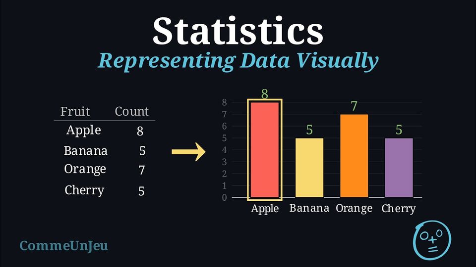
Once data is organised in a table, we can create graphs to see the patterns visually. Bar charts are excellent for comparing the numbers of answers (the frequencies), while pie charts are best for showing proportions.
Definition — Bar Chart
A bar chart uses rectangular bars where the height of each bar represents its frequency. It can be used for qualitative data and for discrete quantitative data. - For qualitative (categorical) data, each bar represents a distinct category (e.g., “Maths”, “Science”). The bars are typically drawn with gaps between them to show the categories are separate.
- For quantitative (numerical) data, each bar represents a specific number (e.g., a score of “3”, or “4 siblings”). The numbers are placed in order along the horizontal axis.
Definition — Line Plot
A line plot (also called a dot plot) shows numerical data using marks above a number line. Each data value is shown by one dot placed above its number; dots for the same value are stacked. A line plot shows at a glance which values are most common and how the data is spread.
Column Graphs and Dot Plots
When its bars stand upright, a bar chart is also called a column graph: one column for each category, as high as its frequency. A dot plot shows the same frequencies with dots: one dot for each answer to the survey, the dots of one category stacked in a column. The line plot is a dot plot for numerical data; a dot plot can just as well be drawn for categories. Here is the “Favourite Subject” survey as a dot plot: counting the dots of each column gives back the frequencies \(8\), \(5\), \(7\) and \(5\) of its bar chart. 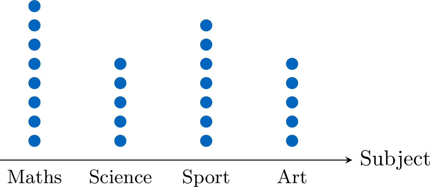
In both graphs, the tallest column shows the mode: Maths.
Skills to practice
- Drawing Column Graphs and Dot Plots
IV.2
Drawing Pie Charts
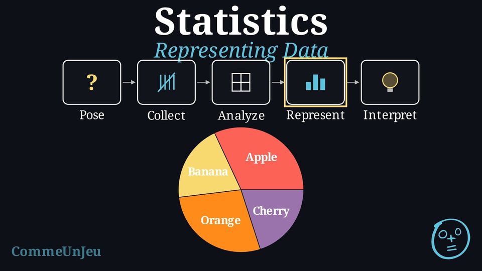
Definition — Angle of a Sector
A pie chart shows the proportion of each category as a slice of a circle (a sector). If the relative frequency of a category is written as a decimal (a percentage is first converted: \(32\pourcent = 0.32\)), the angle for its slice is calculated as: $$ \text{Angle} = \text{Relative Frequency} \times 360^\circ. $$ Example
Draw a pie chart for our “Favourite Subject” survey data (Total = 25 students). | Subject | Frequency | Relative Frequency |
| Maths | 8 | \(32\pourcent\) |
| Science | 5 | \(20\pourcent\) |
| Sport | 7 | \(28\pourcent\) |
| Art | 5 | \(20\pourcent\) |
First, calculate the angle for each slice: 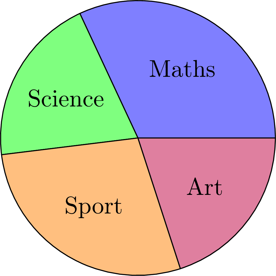
- Maths: \(0.32 \times 360^\circ \approx 115^\circ\)
- Science: \(0.20 \times 360^\circ = 72^\circ\)
- Sport: \(0.28 \times 360^\circ \approx 101^\circ\)
- Art: \(0.20 \times 360^\circ = 72^\circ\)
Skills to practice
- Drawing a Pie Chart
IV.3
Measurements as a Set of Points
Method — Representing Measurements by a Set of Points
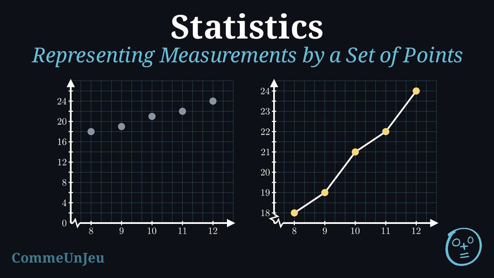
When one quantity is measured while another varies, the pairs of numbers are placed on two axes: each row of the table becomes one point. - Draw two perpendicular axes. Put the quantity that depends on the other on the vertical axis, and the other one (often the time) on the horizontal axis. Name each axis and give its unit.
- Look at the largest value of each column, and pick a scale so that it fits on the sheet. The two axes need not have the same scale.
- Choose where each axis starts: it does not have to be \(0\). If every measurement is between \(18\) and \(25\), starting the vertical axis at \(18\) spreads the points out; a zigzag on the axis marks the cut.
- Place one point per row of the table. Joining the points in order with straight segments gives a line graph.
Example
The temperature of a classroom was measured every hour of a morning. | Time (h) | \(8\) | \(9\) | \(10\) | \(11\) | \(12\) |
| Temperature (°C) | \(18\) | \(19\) | \(21\) | \(22\) | \(24\) |
The times run from \(8\) to \(12\), the temperatures from \(18\) to \(24\). Starting the vertical axis at \(18\) rather than at \(0\) spreads the five points over the whole height instead of crushing them at the top; a zigzag at the bottom of the vertical axis marks the cut. 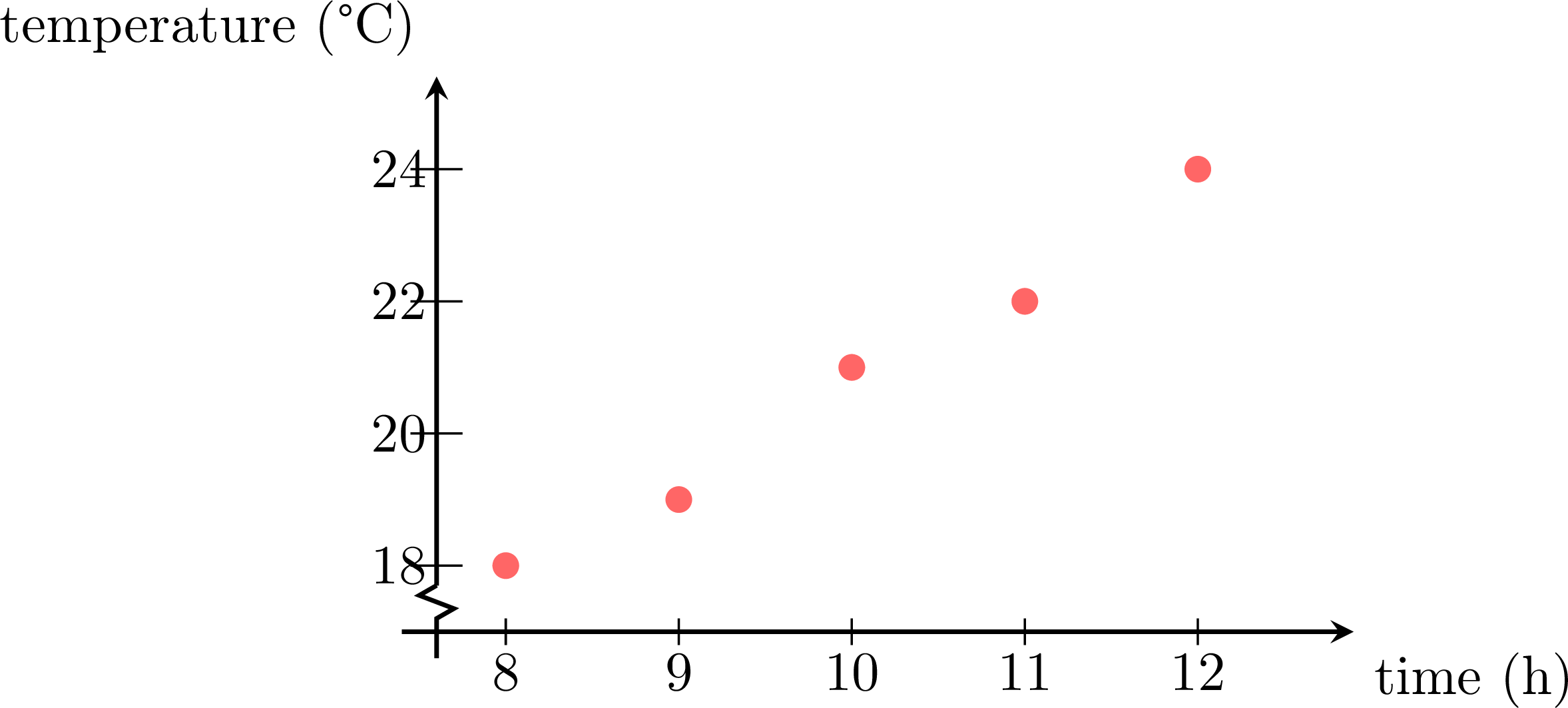
The points rise from left to right: the room warms up through the morning.
Skills to practice
- Representing Measurements by a Set of Points
V
Interpreting Data
V.1
Drawing Conclusions from Data
Method — A Method for Interpreting Data
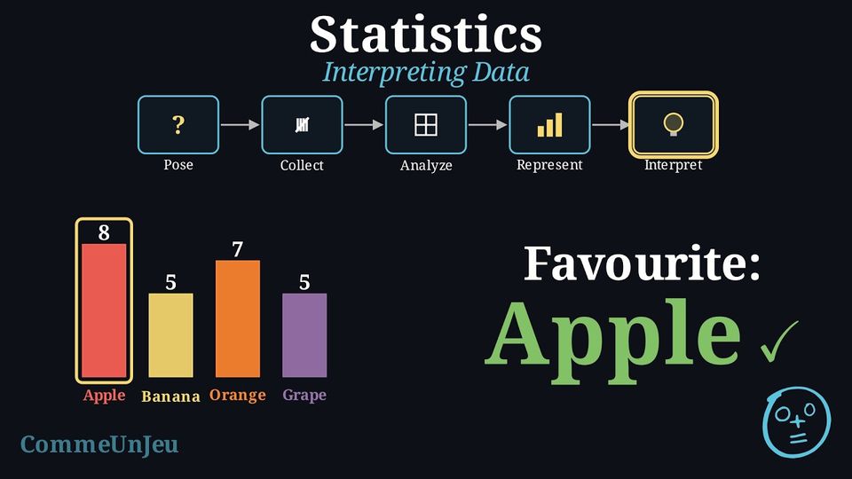
Interpretation is the final and most important step: it tells the story that the data tell. These steps lead to a strong interpretation. - State the Main Findings: Start by describing the most obvious points. What is the most popular category (the mode)? What is the least popular?
- Make Comparisons: Use comparative words (e.g., “more than”, “less than”, “twice as many”) to compare different categories. Perform simple calculations if needed.
- Use Specific Data as Evidence: Support each statement with numbers: the frequencies, or the proportions as percentages, from the table or the chart.
- Draw a Conclusion: Write a concluding sentence that directly answers the original statistical question.
- Reflect and Ask New Questions: Think about what the data do not tell. Does this result apply to the whole school, or just to the class? What could be investigated next?
Example — Interpreting the “Favourite Subject” Survey
We apply the 5-step method to interpret the results from our survey on favourite subjects. | Subject | Frequency | Proportion (\(\pourcent\)) |
| Maths | 8 | \(32\pourcent\) |
| Science | 5 | \(20\pourcent\) |
| Sport | 7 | \(28\pourcent\) |
| Art | 5 | \(20\pourcent\) |
- Main Findings: The data shows that Maths is the most popular subject. The least popular subjects are Science and Art, which are tied.
- Comparisons: More students chose Maths (8) than Sport (7). The number of students who prefer Science is the same as the number who prefer Art (5).
- Evidence: Maths is the favourite for 32\(\pourcent\) of the class, the most chosen subject (the mode), just ahead of Sport (8 against 7).
- Conclusion: In conclusion, based on our survey of 25 students, the favourite subject in this class is Maths.
- Reflection: This conclusion only applies to our class of 25 students. A new question for a future investigation could be: “Is Maths also the favourite subject in the entire school?”
Shares, not numbers. These two pie charts look exactly the same: in both, reading takes a quarter of the disc. But the first one is about a class of \(20\) pupils and the second about a school of \(100\) pupils. A quarter of \(20\) is \(5\) pupils; a quarter of \(100\) is \(25\) pupils. The same sector can stand for very different numbers: shares can be compared on the discs, but to compare numbers between two pie charts, look at their totals first. 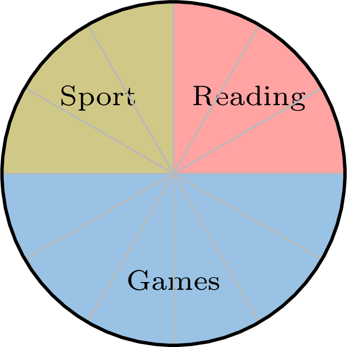
Method — Making a Choice by Filtering a Table
A table often holds more than is needed. Choosing means keeping only the rows that satisfy a criterion, then comparing what is left. - Say in words what is wanted, and turn it into a criterion: one column, one condition.
- Go through the table row by row and keep only the rows that satisfy it.
- Among the rows kept, compare on the column that decides, and name the answer.
- Check that no kept row was forgotten, and that no rejected row satisfied the criterion.
Example
Four trains go from the town to the sea. | Train | Departure | Duration | Price |
| A | \(7{:}10\) | \(3\) h \(05\) min | \(\dollar 34\) |
| B | \(9{:}40\) | \(2\) h \(50\) min | \(\dollar 52\) |
| C | \(12{:}15\) | \(3\) h \(20\) min | \(\dollar 29\) |
| D | \(16{:}05\) | \(2\) h \(45\) min | \(\dollar 61\) |
The first criterion is “arrives before \(13{:}00\)”. The table does not give the arrival, so it is computed for each train, departure plus duration: $$\begin{aligned} A &: 7{:}10 + 3\,\text{h}\,05\,\text{min} = 10{:}15 && \text{(kept)} \\
B &: 9{:}40 + 2\,\text{h}\,50\,\text{min} = 12{:}30 && \text{(kept)} \\
C &: 12{:}15 + 3\,\text{h}\,20\,\text{min} = 15{:}35 && \text{(rejected)} \\
D &: 16{:}05 + 2\,\text{h}\,45\,\text{min} = 18{:}50 && \text{(rejected)} \end{aligned}$$ Two trains are left, so the second criterion, the price, decides between them: \(\dollar 34\) for train \(A\) against \(\dollar 52\) for train \(B\). The answer is train A.
Skills to practice
- Drawing Conclusions from a Table
- Comparing Data Sets with Pie Charts
- Reading Charts and Graphs
- Comparing and Choosing with Data
VI
Going further
Skills to practice
- Conducting a Full Investigation
- Investigating Patterns in Data
- Quiz
Jump to section