International Baccalaureate · MYP 3

Statistics

⌚ ~138 min ▢ 15 blocks ✓ 62 exercises ➣ Prerequisites : Percentages and Money, Statistics, Linear Equations

I Samples and Claims

I.1 Sampling Error and Selection Bias

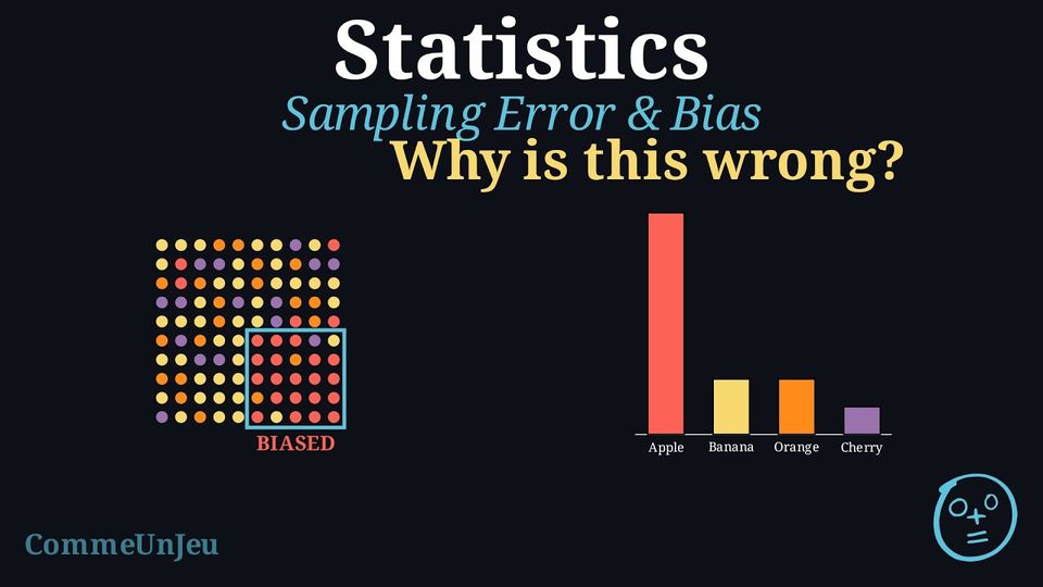
Definition — Representative Sample

A sample is representative when it reflects the whole population: the different groups inside the population appear in the sample in about the same proportions as in the population. A conclusion drawn from a representative sample can reasonably be extended to the whole population. A sample that is biased leans toward one type of answer and does not reflect the population, so its conclusion cannot be trusted.

One of the most common ways to collect information about a large group is to use a sample. For a sample to be meaningful, it must fairly represent the entire population. Two key challenges in sampling are avoiding bias and choosing a sample size that is large enough to capture the population’s diversity.

Selection bias: A famous example of biased sampling is the Literary Digest poll before the 1936 US presidential election. The magazine sent millions of surveys using telephone books and car registration lists. But during the Great Depression, many people could not afford phones or cars. This led to a sample heavily biased towards wealthier citizens, who at the time were more likely to vote Republican. Because of this bias, the poll incorrectly predicted a landslide win for Alfred Landon, while Franklin D. Roosevelt actually won by a wide margin.
Sample size: In a school of $1\,000$ students, $500$ walk to school, that is $50\pourcent$. Two groups of students are chosen at random and asked. In a sample of $10$ students, $7$ walk to school, that is $70\pourcent$; in a sample of $200$ students, $104$ walk, that is $52\pourcent$. Both samples are chosen fairly, but the small one is far from the true $50\pourcent$, by chance alone: with $10$ students, one walker more or fewer changes the result by $10\pourcent$; with $200$ students, by only $0.5\pourcent$.

Report an error

Definition — Sampling Error

A result calculated from a sample usually differs from the true value for the entire population. Sampling error is the part of that difference that comes from chance alone. It exists simply because a sample is a part of the whole, not the whole itself, and because the individuals chosen by chance will usually differ somewhat from the population as a whole.

Definition — Selection Bias

Selection bias is a systematic error that occurs when the method of selecting a sample causes it to be unrepresentative of the population. Unlike random sampling error, bias pushes the results in a specific direction and does not disappear just by increasing the sample size.

Example

An investigation asks: “What is the favourite subject of the students at this school?” To collect data, only the students of one maths class are surveyed.
This is a biased sample.

The population is all the students of the school.
The sample is only the students of this maths class.

The results are likely to be biased because this sample is not representative of the whole school. For example, students in a maths class might be more likely to choose Maths as their favourite subject than students selected from an art class or from the whole school. Students from other year levels or special programmes may also have very different preferences, but their opinions are completely left out. Therefore, the conclusion cannot be generalised to the whole school.

Method — Reducing Error in Sampling

To ensure a survey's results are as accurate as possible, statisticians use two main strategies:

Use Random Sampling: To reduce selection bias, every member of the population should have an equal chance of being chosen for the sample. This is the foundation of reliable surveying (though a good design requires more than equal chances alone).
Increase the Sample Size: As the sample size gets larger, it is more likely to accurately reflect the diversity of the population, and the random sampling error generally decreases. However, increasing the sample size alone does not remove selection bias if the method of selection is already flawed.

Skills to practice

Identifying Flaws in Statistical Reasoning

I.2 Evaluating Statistical Claims

A conclusion drawn from a survey describes the people surveyed; it extends to a whole population only insofar as the sample is representative — a census of the population would be needed to be certain.

Report an error

Method — Critically Evaluating a Statistical Claim

When presented with a statistical claim, a critical evaluation should focus on two key areas:

Validity of the Data Collection: Was the sample representative of the target population, or could selection bias have influenced the results? Was the sample size adequate to support the conclusion? Were the questions neutral and unambiguous to avoid measurement error?
Scope of the Conclusion: Does the conclusion overgeneralise the findings? A common error is to mistake a trend within a specific sample for a universal truth. A descriptive statistic (like a mean) summarises a group but does not apply to every individual within that group.

Example — Evaluating a Claim

Claim: “Girls are better at maths than boys.”
Evidence Provided: A study of one class found that the girls' mean test score was 87$\pourcent$, while the boys' mean was 75$\pourcent$.
Critical Evaluation: The general claim is not justified by the evidence provided.

Limitation of the Sample (Generalisation): The sample consists of only one class. It is not random and is too small to be considered representative of the entire population of “all girls” and “all boys”. The conclusion cannot be generalised beyond this specific group.
Misinterpretation of Averages: The mean describes the central tendency of a group, not the performance of individuals. Even with a higher mean for the girls, some boys may well have scored higher than some girls — the means alone do not determine individual results. The claim “Girls are better” is an overgeneralisation that is easily read as true of every individual.

A more accurate and statistically valid conclusion is: “In the class that was studied, the mean score for girls was higher than the mean score for boys.”

Skills to practice

Evaluating Statistical Claims

II Frequency Tables and Summaries

II.1 Finding a Missing Frequency

Example

The $32$ members of a club each chose one sport. One frequency is missing.

Sport	Football	Basketball	Swimming	Dance	Total
Frequency	11	7	?	6	32

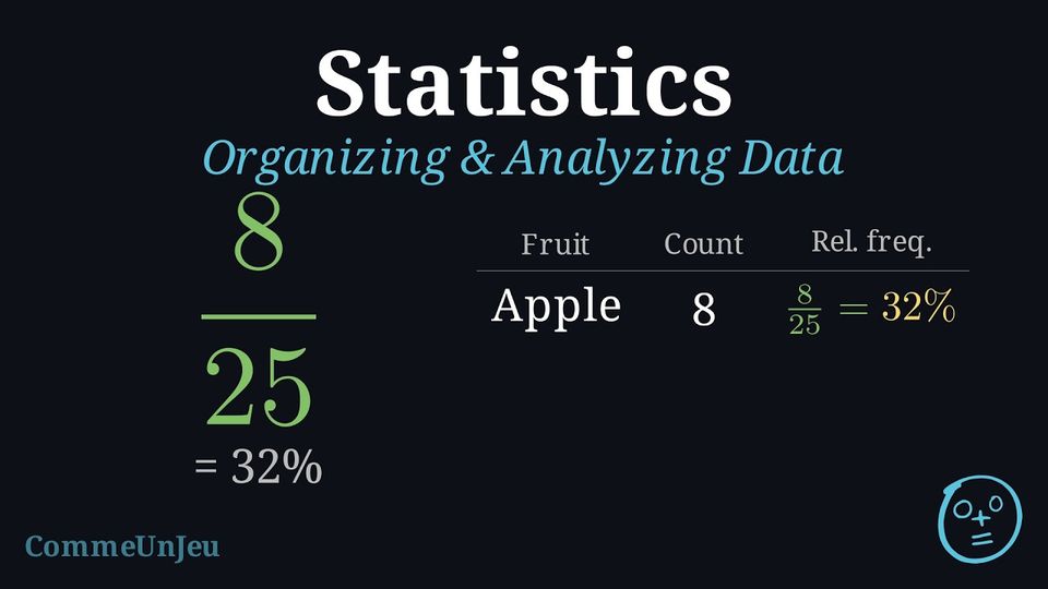
Determine the missing frequency, then the relative frequency of swimming.

Answer

The frequencies add up to the total, so the missing one is the total minus the known ones: $$32 - (11 + 7 + 6) = 32 - 24 = \textcolor{colordef}{8}.$$ Check: $11 + 7 + 8 + 6 = 32$. The relative frequency of swimming is $\dfrac{8}{32} = 0.25 = 25\pourcent$.

Skills to practice

Finding a Missing Frequency in a Table

II.2 The Mean from a Frequency Table

Definition — Weighted Mean

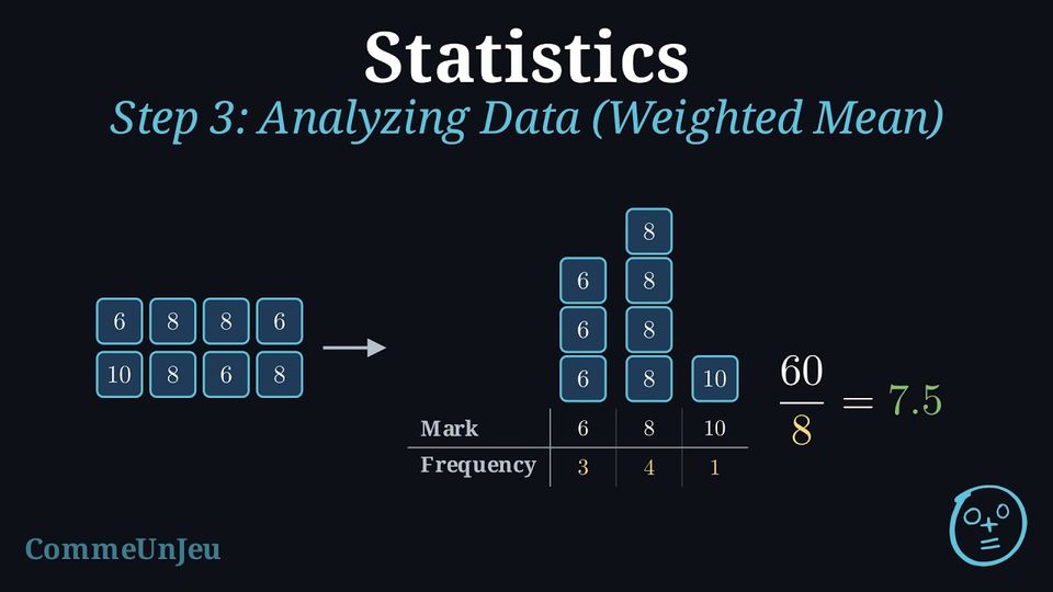
When a value appears several times in a dataset, it is wasteful to add it one by one. Multiply each value by its frequency (the number of times it appears), add these products, then divide by the total frequency: $$\bar{x} = \dfrac{n_1 \times x_1 + n_2 \times x_2 + \dots}{n_1 + n_2 + \dots}$$ The mean computed this way is called the weighted mean: each value is weighted by its frequency.

Method — Computing a Weighted Mean from a Table

Multiply each value by its frequency.
Add all these products.
Divide by the total frequency — the sum of the frequencies, not the number of columns of the table.

Example

Here are the marks of Lea's last eight vocabulary quizzes, as they came: $6, 8, 8, 6, 10, 8, 6, 8$. Group the repeated values in a table, then compute the mean.

Answer

The value $6$ appears $3$ times, $8$ appears $4$ times and $10$ appears once:

Mark	6	8	10
Frequency	3	4	1
Product	18	32	10

$$\bar{x} = \dfrac{3 \times 6 + 4 \times 8 + 1 \times 10}{3+4+1} = \dfrac{18+32+10}{8} = \dfrac{60}{8} = \textcolor{colorprop}{7.5}$$ Grouping the raw data first turns a long sum into a short weighted mean — same result, less work.

Example

Here are the marks (out of 20) of a class at the last test.

Mark	8	10	12	15
Frequency	3	5	8	4

Compute the mean mark of the class.

Answer

Each mark is multiplied by its frequency, and the total frequency is $3+5+8+4 = 20$ students:

Mark	8	10	12	15
Frequency	3	5	8	4
Product	24	50	96	60

$$\bar{x} = \dfrac{3 \times 8 + 5 \times 10 + 8 \times 12 + 4 \times 15}{3+5+8+4} = \dfrac{24+50+96+60}{20} = \dfrac{230}{20} = \textcolor{colorprop}{11.5}$$ The mean mark of the class is $11.5$ out of $20$.

Example

This bar chart shows how many books the students of a class read last month.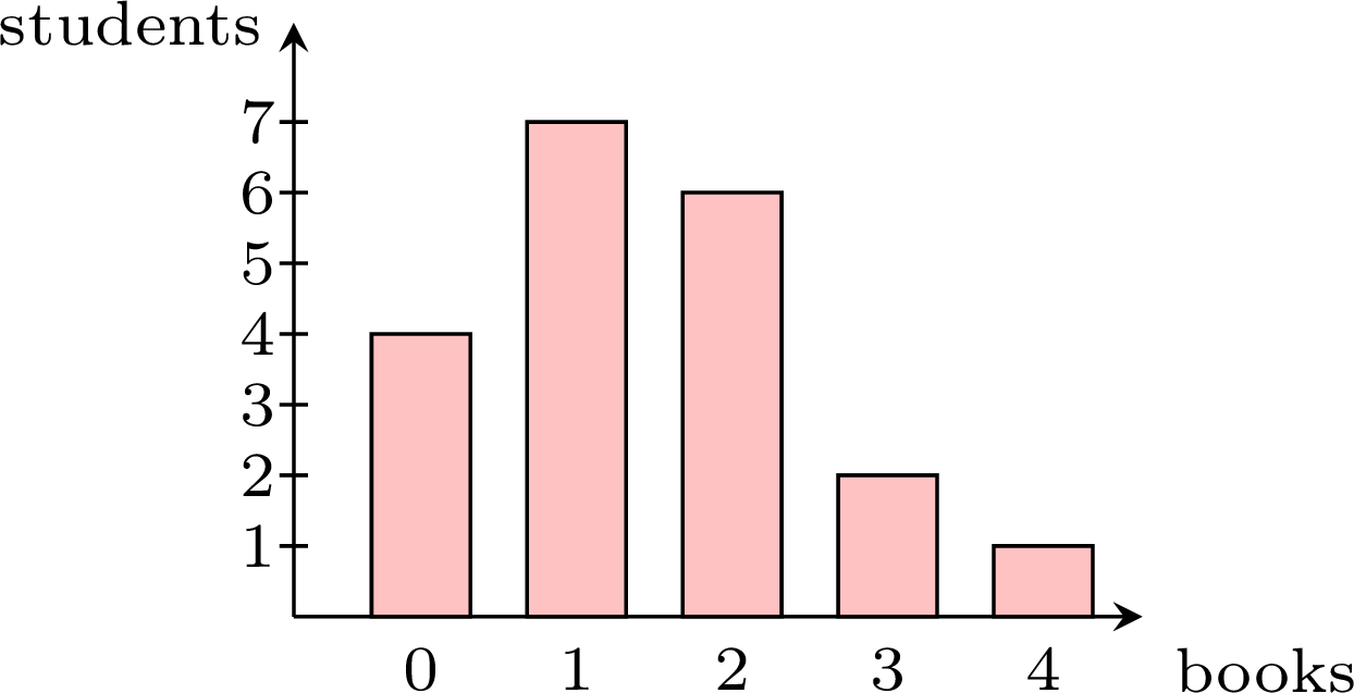

Compute the mean number of books read per student.

Answer

The heights of the bars give the frequencies — $4+7+6+2+1 = 20$ students in total:

Books	0	1	2	3	4
Frequency	4	7	6	2	1
Product	0	7	12	6	4

$$\bar{x} = \dfrac{4 \times 0 + 7 \times 1 + 6 \times 2 + 2 \times 3 + 1 \times 4}{20} = \dfrac{0+7+12+6+4}{20} = \dfrac{29}{20} = \textcolor{colorprop}{1.45}$$ On average, each student read $1.45$ books — the mean does not have to be a whole number, even when every value is a whole number.

Skills to practice

Calculating the Mean from a Frequency Table
Combining Groups and Working Backwards from the Mean

II.3 Cumulative Frequency and the Median

Definition — Cumulative Frequency

In a frequency table, the cumulative frequency of a value is the number of data points less than or equal to that value. It is obtained by adding the frequencies from the smallest value up to that value; the last cumulative frequency is the total number $N$ of data points.

Example

The marks (out of 20) of a class are gathered in the table below.

Mark	8	10	12	14	16
Frequency	2	3	4	7	5

Build the row of cumulative frequencies.
How many pupils scored at most 12?
Use the cumulative frequencies to find the median mark.

Answer

Adding the frequencies step by step:

Mark 8 10 12 14 16

Frequency 2 3 4 7 5

Cumulative frequency 2 5 9 16 21
The cumulative frequency of 12 is $9$: nine pupils scored at most 12.
There are $N = 21$ marks (odd), so the median is the $11^{\text{th}}$ ordered mark. The $11^{\text{th}}$ ordered mark falls at 14 (since $9 < 11 \leq 16$): the median mark is $14$.

The median is not the mark in the middle of the table ($12$): it is the middle of the ordered list of the 21 marks, and here the large frequencies sit on the high marks.

Method — Finding the Median from a Frequency Table

Find the middle position or positions in the list of the $N$ data points ordered from the smallest to the largest, where the values are numbered $1$, $2$, …, $N$;
- if $N$ is odd, the median is the value in position $\dfrac{N + 1}{2}$;
- if $N$ is even, the median is the mean of the values in positions $\dfrac{N}{2}$ and $\dfrac{N}{2} + 1$.
Build the row of cumulative frequencies.
Locate each position: the value in position $r$ is the first value whose cumulative frequency is greater than or equal to $r$.
When $N$ is even, the two middle positions fall on two different values exactly when a cumulative frequency equals $\dfrac{N}{2}$; the median is the mean of these two values. Otherwise, both middle positions fall on the same value, which is the median.

Example

The table gives the number of books borrowed from the library last month by the $24$ pupils of a class.

Books	0	1	2	3	4	5
Frequency	5	7	3	4	2	3

Find the median number of books borrowed.

Answer

$N = 24$ is even, so the median is the mean of the values in positions $12$ and $13$. The cumulative frequencies are:

Books	0	1	2	3	4	5
Frequency	5	7	3	4	2	3
Cumulative frequency	5	12	15	19	21	24

Position $12$: $5 < 12 \leq 12$, so the $12^{\text{th}}$ value is $1$ (the cumulative frequency of $1$ is exactly $12$).
Position $13$: $12 < 13 \leq 15$, so the $13^{\text{th}}$ value is $2$.

$$\text{median} = \frac{1 + 2}{2} = 1.5 \text{ books.}$$ The cumulative frequency of $1$ is exactly $\dfrac{24}{2} = 12$: half of the pupils borrowed at most $1$ book, the other half $2$ or more. The median, $1.5$, is not one of the values of the table; it is not the middle of the row of values either ($2.5$), because the large frequencies sit on the small values.

Skills to practice

Reading Cumulative Frequency Tables
Finding the Median from a Frequency Table

III Displaying Data

III.1 Splitting the Stems

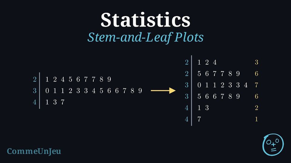
Definition — Stem-and-Leaf Plot

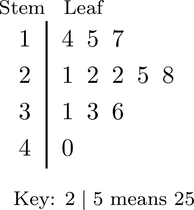
A stem-and-leaf plot (or stemplot) displays numerical data by splitting each value into a stem, made of all its digits except the last one, and a leaf, its last digit; a one-digit value such as $8$ has the stem $0$.

The stems are written once each, in increasing order, in a column to the left of a vertical line.
Each value writes its leaf in the row of its stem, the leaves being evenly spaced.
In an ordered stem-and-leaf plot, the leaves of each row are in increasing order.
A key, such as “$2 \mid 5$ means $25$”, gives the place value of the leaves. For decimals, the key gives the place value of the leaf: with the key “$2 \mid 4$ means $0.24$”, the stem is the tenths digit and the leaf the hundredths digit.

The ordered stem-and-leaf plot below shows the ages of the $12$ players of a volleyball club: the row $2 \mid 1\ 2\ 2\ 5\ 8$ stands for the ages $21$, $22$, $22$, $25$ and $28$.

Definition — Split Stems

When a few stems carry many leaves, each stem can be split into two rows: the first row takes the leaves $0$ to $4$, the second row the leaves $5$ to $9$. Each row then covers $5$ consecutive values instead of $10$ — for the stem $3$, the values from $30$ to $34$, then from $35$ to $39$ — and the plot has twice as many rows, which shows the shape of the data better. The key is written as before.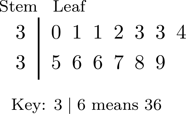

Example

The ordered stem-and-leaf plot gives the marks out of $50$ of $25$ pupils.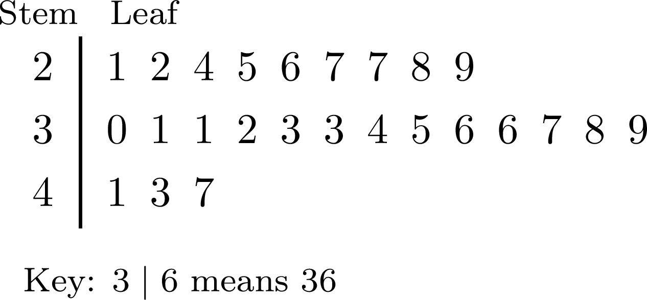

Draw the plot again with split stems, then compare what the two plots show.

Answer

Each stem gets two rows: the leaves $0$ to $4$ in the first, $5$ to $9$ in the second. The row $2 \mid 1\ 2\ 4\ 5\ 6\ 7\ 7\ 8\ 9$ becomes $2 \mid 1\ 2\ 4$ and $2 \mid 5\ 6\ 7\ 7\ 8\ 9$, and so on.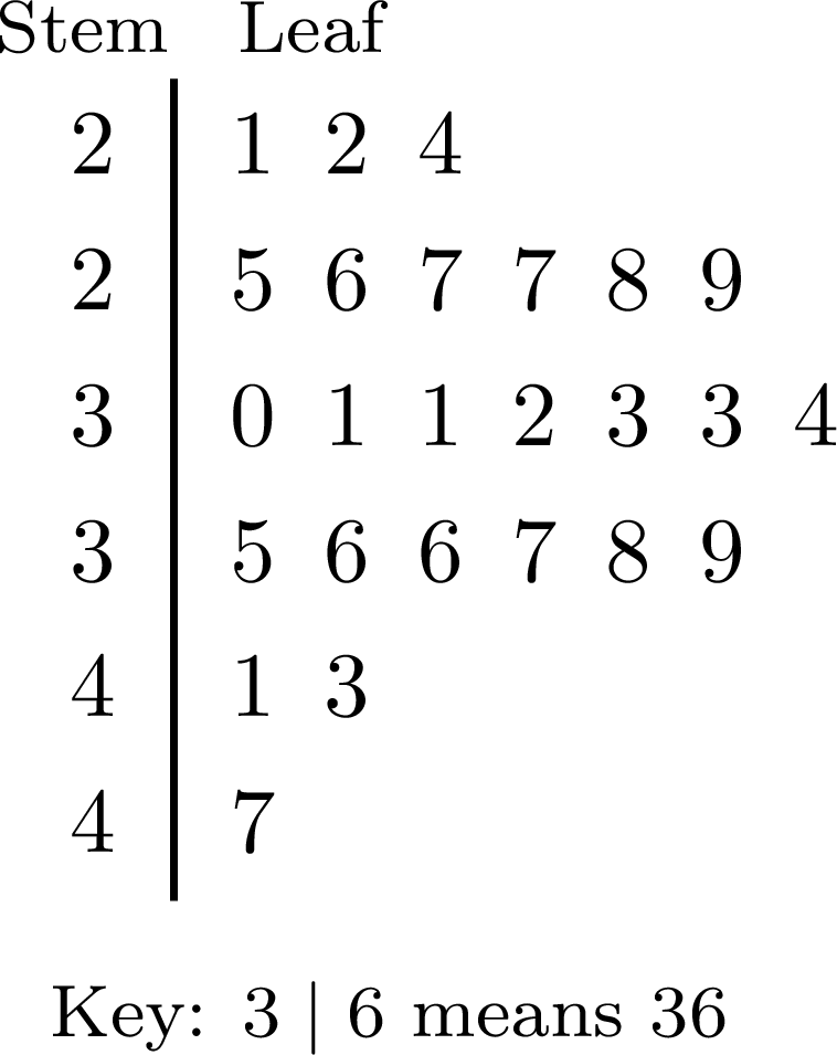

The plot still has $3 + 6 + 7 + 6 + 2 + 1 = 25$ leaves. With three rows, the first plot only shows that most marks are in the thirties. With six rows, the lengths rise from $3$ to $7$ leaves, then fall to $1$: the marks gather around $30$ to $34$, with about as many marks on each side, and a few high marks in the forties.

Choosing the Stems

A stem-and-leaf plot is easiest to read with about $5$ to $10$ rows. With too few rows, all the leaves pile up in one or two rows and the shape is lost; with too many, each row holds one leaf or none. Splitting the stems doubles the number of rows. Each row gathers the values of an interval of the same width, $10$ or $5$: a stem-and-leaf plot is already a way of grouping the data, which keeps every value.

Report an error

Skills to practice

Splitting the Stems

III.2 Grouped Data and the Modal Class

Discover

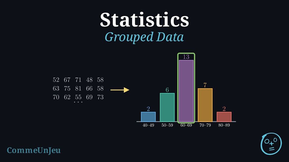
A basketball team scored the following numbers of points in the $30$ matches of its season: $$\begin{aligned}&52,\ 67,\ 71,\ 48,\ 58,\ 63,\ 75,\ 81,\ 66,\ 58,\ 70,\ 62,\ 55,\ 69,\ 73,\\ &64,\ 47,\ 60,\ 78,\ 65,\ 57,\ 68,\ 72,\ 61,\ 84,\ 66,\ 58,\ 74,\ 63,\ 69.\end{aligned}$$ Among these $30$ scores there are $25$ different values, most of them appearing once.
A frequency table with one row for each value would have $25$ rows. How could the scores be organised so that a short table shows how they are spread?

Answer

The scores can be counted by tens: the scores from $40$ to $49$, from $50$ to $59$, and so on up to $80$ to $89$. Each score falls in exactly one group, and five counts are enough:

Points	$40$–$49$	$50$–$59$	$60$–$69$	$70$–$79$	$80$–$89$
Matches	$2$	$6$	$13$	$7$	$2$

The short table shows at once that the team most often scores between $60$ and $69$ points, and rarely below $50$ or above $80$. Such groups of values are called classes.

Definition — Classes and Grouped Frequency Table

When data take many different values, they are grouped into classes (or class intervals) of the same width.

The class $20 \le x < 30$ contains every value $x$ from $20$ included to $30$ excluded, so that each value belongs to exactly one class: the value $30$ belongs to the next class, $30 \le x < 40$. The width of this class is $30 - 20 = 10$.
For whole-number data, the class $20 \le x < 30$ holds the values $20$, $21$, …, $29$, and is also written $20$–$29$.
The frequency of a class is the number of values in it. A grouped frequency table lists the classes in increasing order, with their frequencies; its total is the number of values.

Method — Building a Grouped Frequency Table

Find the smallest and the largest values.
Choose the width of the classes — $5$, $10$, $20$, …— so that there are enough classes to show the shape and enough values in each class: often $5$ to $10$ classes, fewer for a small set of data. The first class starts at a multiple of the width not larger than the smallest value.
Write the classes in increasing order, with no gap and no overlap between them.
Go through the data once, making a tally mark in the row of the class of each value.
Count the tally marks of each class, and check that the frequencies add up to the number of values.

Definition — Modal Class

For data grouped into classes of the same width, the modal class is the class with the highest frequency; when several classes share the highest frequency, each of them is a modal class. It shows where the values are the most concentrated. It is not always the class that contains the mode of the data: a single value that appears several times can lie in another class.

Example

The numbers of text messages sent in one day by $24$ pupils are: $$\begin{aligned}&3,\ 12,\ 25,\ 8,\ 17,\ 31,\ 14,\ 6,\ 22,\ 19,\ 27,\ 11,\\ &35,\ 16,\ 9,\ 21,\ 13,\ 18,\ 28,\ 5,\ 15,\ 24,\ 38,\ 10.\end{aligned}$$

Build a grouped frequency table with classes of width $10$, starting at $0$.
Give the modal class. Do these data have a mode?

Answer

The values go from $3$ to $38$: four classes of width $10$ cover them. One tally mark is made for each value, in the order of the list.

Messages Tally Frequency

$0 \le x < 10$ $5$

$10 \le x < 20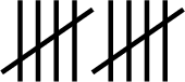$ $10$

$20 \le x < 30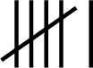$ $6$

$30 \le x < 40$ $3$

Total $24$

The value $10$ goes in the class $10 \le x < 20$, not in $0 \le x < 10$. Check: $5 + 10 + 6 + 3 = 24$.
The highest frequency is $10$: the modal class is $10 \le x < 20$. The data have no mode, since every value appears only once; the modal class still shows where the values are the most concentrated.

Skills to practice

Checking Split Stems and Classes
Building and Reading Grouped Frequency Tables

III.3 Column Graphs of Grouped Data

Method — Drawing a Column Graph of Grouped Data

For whole-number data grouped into classes of the same width:

Write the classes along the horizontal axis, in increasing order, one label under each column, such as $20$–$29$.
Mark the vertical axis with the frequencies, from $0$, in equal steps.
Draw one column per class, all of the same width, whose height is the frequency of the class.
Name the two axes and give the graph a title.

The columns are separate, as in a bar chart: each one stands for a group of whole numbers.

Example

The points scored by the basketball team of the opening problem are grouped in the table below.

Points	$40$–$49$	$50$–$59$	$60$–$69$	$70$–$79$	$80$–$89$
Matches	$2$	$6$	$13$	$7$	$2$

Draw a column graph of this table, and give the modal class.
In what percentage of its matches did the team score at least $70$ points?

Answer

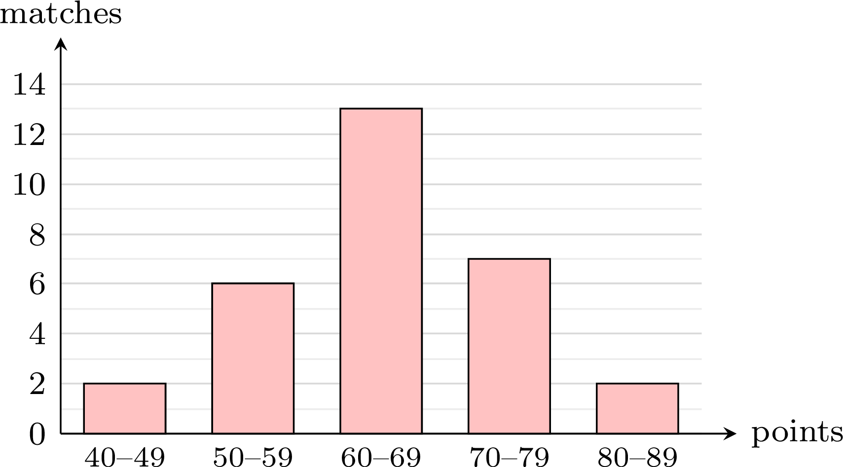
One column per class, on a vertical scale from $0$ in steps of $2$: The tallest column is that of the class $60$–$69$, with $13$ matches: it is the modal class, $60 \le x < 70$.
At least $70$ points means the classes $70$–$79$ and $80$–$89$: $7 + 2 = 9$ matches out of $30$. $$\frac{9}{30} \times 100\pourcent = 30\pourcent.$$

What Grouping Hides

A grouped table is shorter, but the exact values are lost. In the scores of the basketball team, the value $58$ appears three times, more than any other: the mode is $58$, in the class $50$–$59$, while the modal class is $60$–$69$. From the table alone, the mode cannot be found — not even its class — and neither can the exact median, the exact smallest and largest values, or the range: the table only tells in which class the middle of the list lies, and in which classes the smallest and the largest values lie. A stem-and-leaf plot groups the values in the same way while keeping them all.

Report an error

Skills to practice

Reading Column Graphs of Grouped Data
Drawing and Using Grouped Displays

IV Going further

Skills to practice

Problems
Conducting a Full Investigation
Investigating Patterns in Frequency Tables
Quiz

Points	\(40\)–\(49\)	\(50\)–\(59\)	\(60\)–\(69\)	\(70\)–\(79\)	\(80\)–\(89\)
Matches	\(2\)	\(6\)	\(13\)	\(7\)	\(2\)

Messages	Tally	Frequency
\(0 \le x < 10\)		\(5\)
\(10 \le x < 20\)		\(10\)
\(20 \le x < 30\)		\(6\)
\(30 \le x < 40\)		\(3\)
Total		\(24\)

Points	\(40\)–\(49\)	\(50\)–\(59\)	\(60\)–\(69\)	\(70\)–\(79\)	\(80\)–\(89\)
Matches	\(2\)	\(6\)	\(13\)	\(7\)	\(2\)