How to Teach Functions

This guide is for teachers who use CommeUnJeu with a class, from the first function machine in PYP 4 to the function written \(f : x \longmapsto f(x)\) in MYP 5. One machine carries the whole path: a number goes in, the machine applies its rule, and exactly one output comes out. The drawing of the machine changes with the age of the pupils, the machine does not. The guide shows that machine as the lessons show it, follows it year by year with the figures and videos of the chapters, and says where it is not enough. In each chapter you will find:

• most sections open with a short video (this guide shows them too, at the head of the passages they belong to);
• the lesson: definitions, methods and worked examples, to project on the board;
• under each section, the skills to practise: groups of exercises corrected at once, each answer followed by a worked correction;
• some exercises are written on paper or on the slate: the pupil draws the machine, passes a number through it, then writes the calculation, and sends a photo of the page to have it corrected.

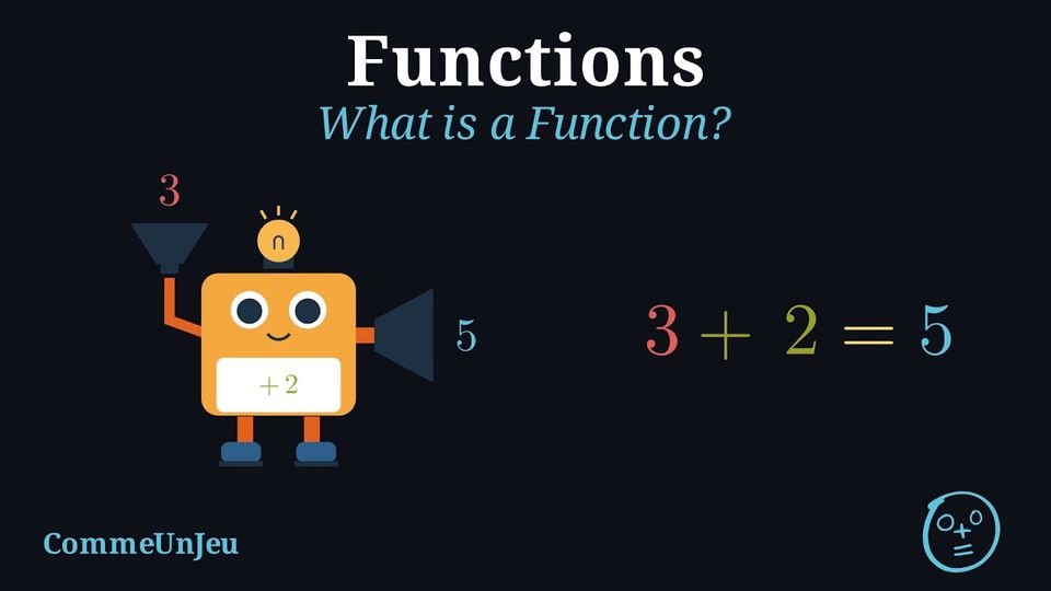
The first definition is already the right one, and the later years only rewrite it: “A function is a rule that takes an input number and gives back exactly one output number. For each input, the function machine always gives the same output and follows the same rule every time.” In PYP 4 the machine is a robot: the rule is written on it, the input goes in at the top, the output comes out at the side. 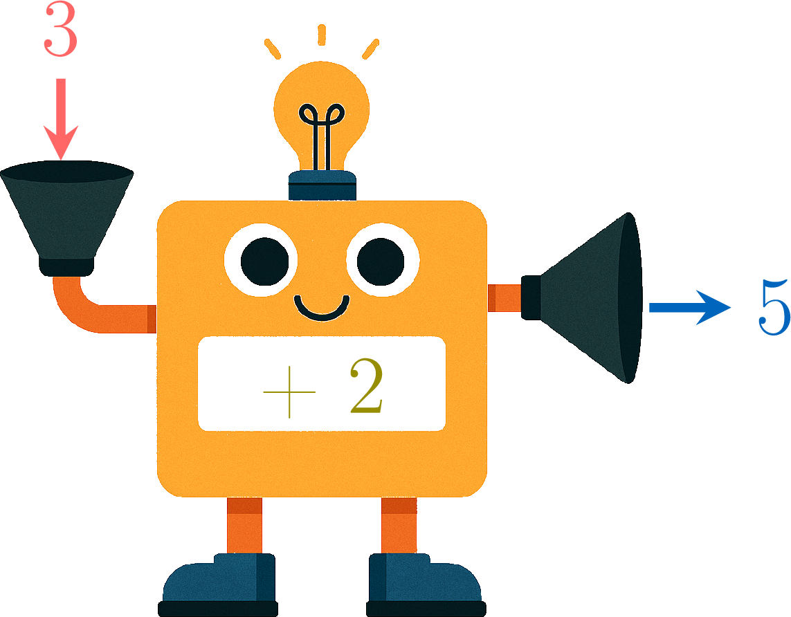The colours do not change from one year to the next: the input in red, the rule in olive, the output in blue. Everything that follows is said on this machine.

• A table of values lists some inputs and their outputs: it is the machine's notebook, not the machine.
• A formula is one way of writing the rule; a function does not need one. A table of steps, read case by case, is a rule too.
• A graph places each pair (input, output) as a point; the machine gives the points, not the line drawn between them.
• Running the machine backwards looks for the inputs that give a known output: zero, one or several inputs, and the machine is still a function.

The word “relation” is kept for something else: the link between two quantities, in a formula or a graph from a situation — the distance and the time of a journey, the side and the perimeter of a square. In MYP 1 and MYP 2 the chapters on line graphs say it in this sense. The course never builds the function as a relation that would be a set of ordered pairs with one more condition: in MYP 5, after the machine definition, a relation is also written as a set of ordered pairs, and multiple-choice questions ask whether a set of pairs is a function; the definition stays the machine's.

The machine is the same from 9 to 16, but a robot is a childish drawing for a pupil of 13. The lessons therefore use three drawings of the same machine — the robot until about 11, the box from about 12, the arrow from about 15 — and show each change once, the two drawings side by side.

• In PYP 4 and PYP 5: the robot, as above.
• In MYP 1 and MYP 2: the box. A rectangle with the rule written inside, an arrow for the input that goes in, an arrow for the output that comes out. In the chapters it first appears with a conversion graph in MYP 1: euros go in, dollars come out. In the IB chapters the box arrives there without the robot beside it. One lesson figure shows the change itself, the robot and the box side by side: show it the day the box appears.
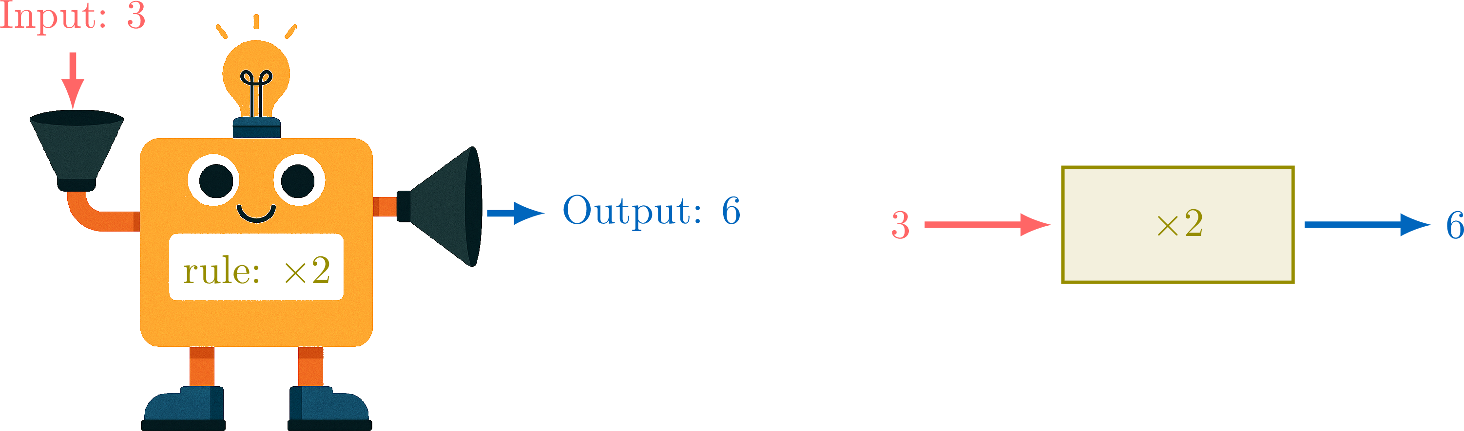
• In MYP 5: the arrow. The box receives a name, \(f\), its output is written \(f(x)\), and the same machine is written on one line, \(f : x \longmapsto f(x)\). The definition of the MYP 5 chapter shows the box and the line side by side:
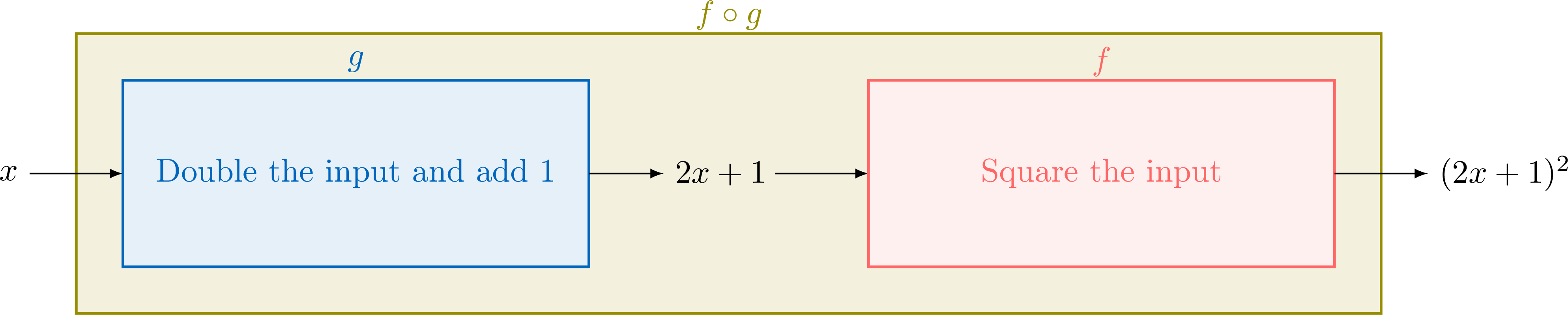
• After 15, the box comes back for composition, and for the inverse function. Two machines in a chain, the output of the first entering the second, are read better drawn than written. The lessons on composition draw them (MYP 5 Extended, Further Functions, and the DP):

Change the drawing, never the machine. When the box replaces the robot, say it is the same machine; when the notation \(f(x)\) appears, say again what it means: the output that the machine \(f\) gives to the input \(x\).

Each chapter takes up the machine where the year before left it, then goes one step further. The table gives the step and the link to the chapter. No MYP 3 or MYP 4 chapter serves these lessons on functions, so the box of MYP 2 and the arrow of MYP 5 are two years apart; MYP 4 meets quadratic functions in a chapter of their own.

Year	Chapter	What is new
PYP 4	Patterns and functions	the robot machine; input, rule, output; In/Out tables; mystery machines
PYP 4	Data Handling	a point for each measurement; what the curve shows, and what it does not
PYP 5	Number sequences and rules	the table of values; machines run backwards; the machine that always answers the same
MYP 1	Line Graphs	relations between two quantities; tables and line graphs; distance-time graphs; conversion graphs, the first box
MYP 2	Coordinates and Straight-Line Graphs	“in terms of”, with the box; from a formula to a graph, and when to join the points
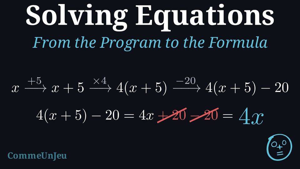
MYP 2	Formulae	a calculation program as machines in a chain; running it backwards
MYP 5	Functions	the box named \(f\), then \(f : x \longmapsto f(x)\); tables; the graph and the vertical line test; images and preimages; deciding whether it is a function; domain and range

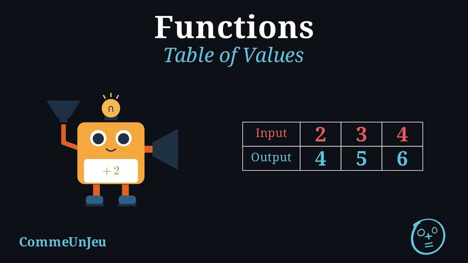
In the lesson. The machine comes with the patterns it already explains: “The In/Out tables of number patterns work in the same way, and so does a table of positions and terms: a position table is an In/Out table, where the position goes in and the term comes out.” In PYP 5 the table of values becomes the machine's notebook: one row of inputs, one row of outputs.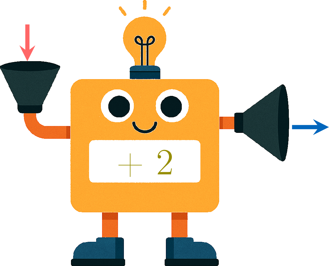

Input	2	3	4
Output	4	5	6

The exercises. Pass a number through the machine; find a rule from a few results; run the machine backwards. The written exercises ask for reasons, on the definition: a machine that answered \(10\) yesterday and \(12\) today for the same input \(5\) is not a function machine; a machine that answers \(7\) to every input is one, even if “it doesn't compute anything”; “multiply by \(2\)” and “add the input to itself” are the same machine, because they give the same output for every input. Watch for the mystery machine played as “guess my rule”. The results of a few inputs can reject a rule, never prove it: the written mystery-machine exercises ask for “a rule that fits” and accept any output consistent with the rule the pupil found. Say it the same way in class.

In the lesson. The PYP 4 chapter on data handling meets the curve the same year as the machine, without the machine yet: two lines that cross make a graph, each measurement becomes one point that carries two readings at once, the month and the temperature. The points are joined in order, and the lesson then says what the curve adds and what it does not. 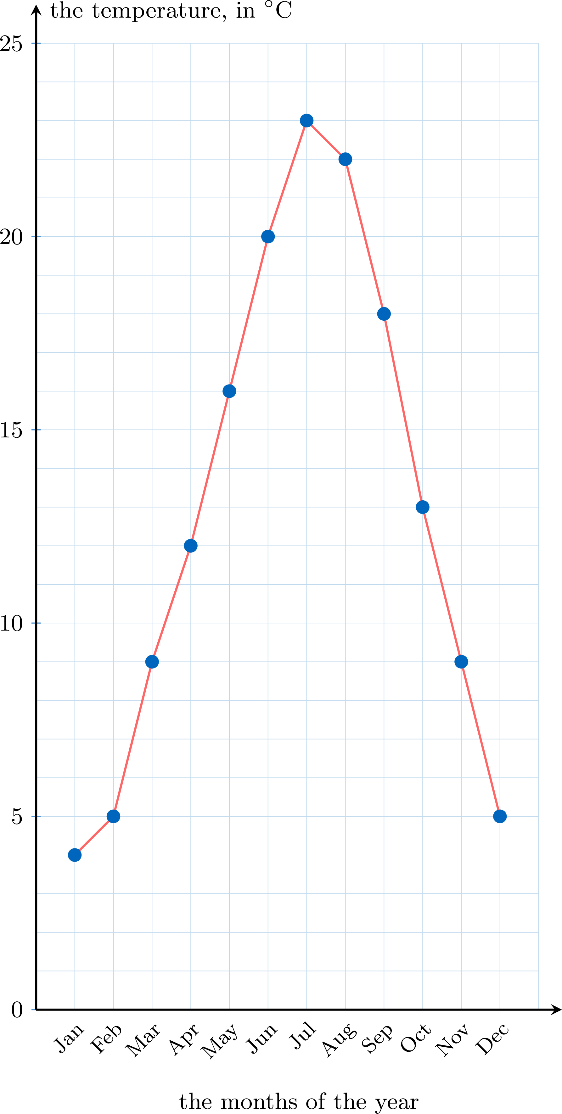Joining the points shows the shape of the change, where it rises and where it falls; but the curve joins the measurements; it does not invent the ones that were never taken. This sentence comes back in MYP 2 and in MYP 5 with formulas: the line drawn between computed points remains a conjecture. The exercises. Reading the curve; placing one point for each measurement of a growing bean plant; and Sami's written exercise, the heart of the chapter: he reads \(20\,^\circ\)C on the line halfway between August and September, and thinks it was measured. Watch for the point read as one of the stacked dots of a line plot, which pupils already know: here it carries two values. Have them say both aloud, “August, \(22\) degrees”, before reading the curve.

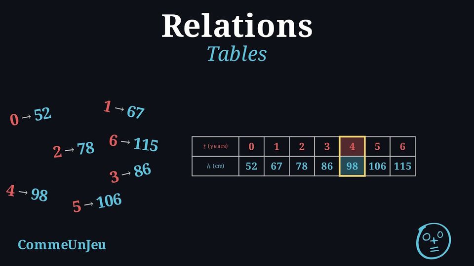
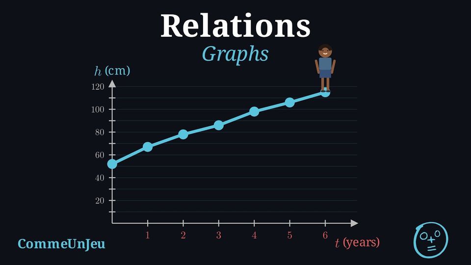
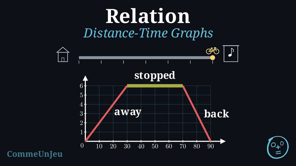
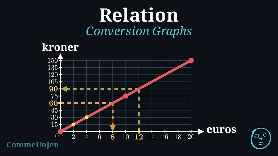
In the lesson. The chapter works on relations between two quantities, in situations: a table, then a line graph, then two kinds of graphs that tell a story. A distance-time graph places the time across and the distance from home up, because the distance depends on the time; each point is read as a sentence. 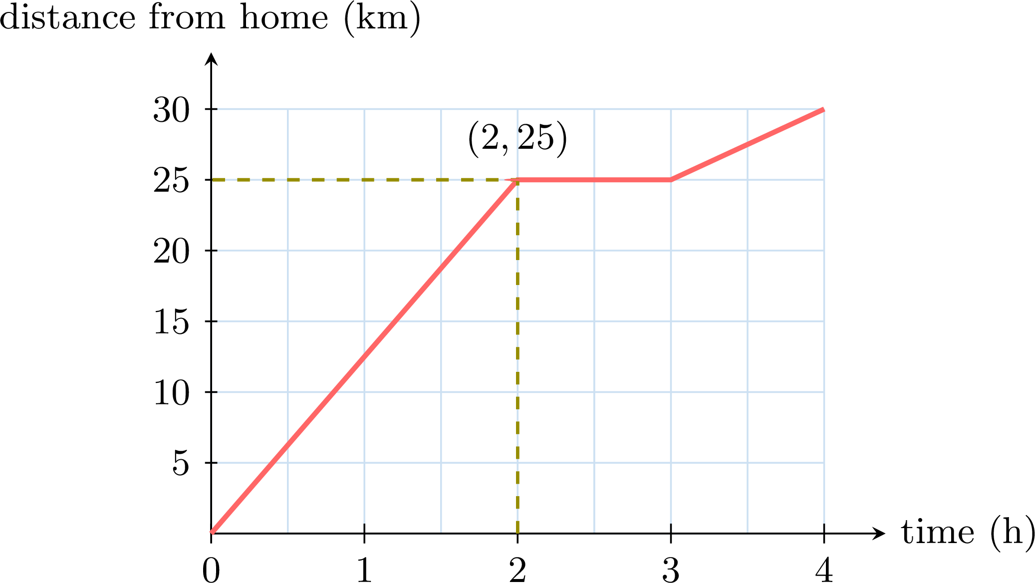The point \((2, 25)\) says “after \(2\) hours, the traveller is \(25\) km from home”. In these graphs the traveller moves straight away from home and comes back the same way, so the distance changes exactly as the traveller moves. The method reads the axes first, then each part: rising, the traveller moves away; flat, the traveller has stopped; falling, the traveller comes back; steeper means faster. And a warning that pupils need: the distance from the start is not the distance travelled — after a return trip the graph is back at \(0\). A conversion graph pairs two equal amounts, and here the box appears: euros go in, the rule “multiply by \(1.2\)” is applied, dollars come out (the figure is in the section on the three drawings). The graph works both ways: reading it from the dollars back to the euros runs the machine backwards, with the rule “divide by \(1.2\)”. Watch for the graph read as a picture of the route: a part that rises is not a hill. Have each point said as a sentence before any part is described.

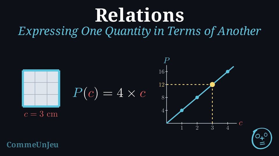
In the lesson. MYP 2 joins the relation and the machine. When each value of the first quantity determines exactly one value of the second, the second is expressed in terms of the first, and the dependence is drawn as a machine: The definition adds what the machine alone does not say, the covariation: “when the side increases by \(1\) cm, the perimeter increases by \(4\) cm, whatever the side”. The method “from a formula to a graph” then says when to join the points: only if the starting quantity can take every value in between (a length, a duration), never for a number of objects; and between two computed points the shape of the line “remains a conjecture; computing one more value with the formula can rule it out, never prove it”. In the chapter on formulae, a calculation program is a chain of small machines, each with its own rule: one starting number gives one result (the section on running the machine backwards comes back to it); the chain then becomes a formula. Watch for the points joined by habit. Ask the question before drawing: can the starting quantity take the values in between?

In the lesson. The opening problem recalls the box of the earlier years, “multiply by \(2\)”, its table, then gives it a name: \(f(\text{input}) = \text{output}\), then \(f(x) = 2x\). The definition follows, with the box and the arrow side by side (see the section on the three drawings): \(f(x)\) is the image of \(x\), and \(x\) an antecedent, also called a preimage, of \(f(x)\). The graph is the set of all the points \((x, f(x))\); “A table of values gives only some of these points: joining them is a conjecture until the rule gives the values in between.” 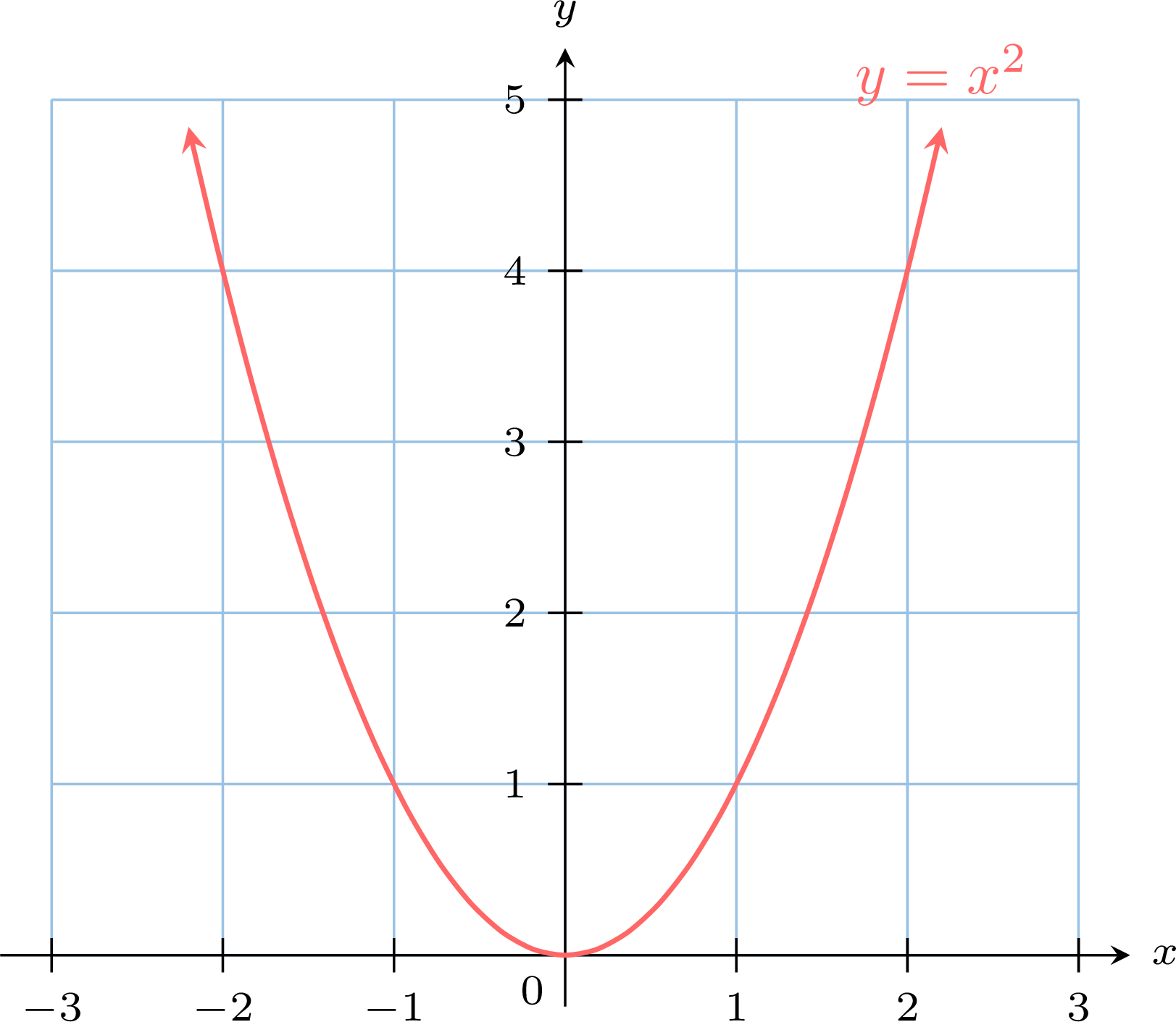The vertical line test reads the definition on the graph: the points of a vertical line all share the same input, so two crossings would give one input two outputs. 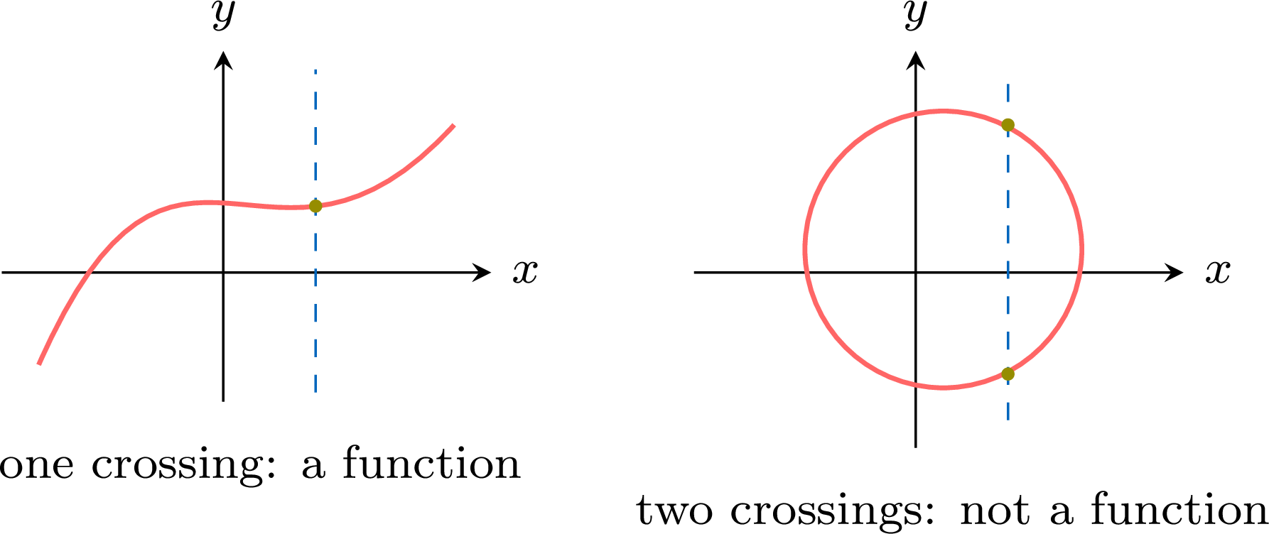Then the image read on the graph, and the preimages, read on the graph, then computed (the section on running the machine backwards). The exercises. Besides the skills of each section, a written group “Deciding Whether a Relation Is a Function” asks for reasons on the definition: arrow diagrams, two tables (one of them constant), two drawings to test with vertical lines. At the end of the chapter, the reasoning group tests Lina's claim that a function may not give the same output twice, and runs the square machine backwards (the task taken apart below). Watch for the vertical line test learnt as a trick. Ask each time what a vertical line is: all the points with the same input.

In the lesson. A machine does not accept every input. Already the definition said it: “The inputs that the machine accepts are the values of \(x\) for which the rule gives an output.” MYP 5 names them: the domain is “the set of all input values \(x\) for which the expression \(f(x)\) is defined […]: the inputs that the machine accepts”; the range is the set of the outputs actually obtained. When a function is given with its domain, that set is its domain; when only the expression is given, the domain is the set of all real numbers for which it is defined. The chapter goes on to the sign of a function, read on its curve, then to sign tables and to transformations. Watch for the box taken as accepting every number. The box has no domain drawn on it; say it each time the rule cannot be applied (a division by zero, the square root of a negative number), and have the pupils write the set of inputs next to the box.

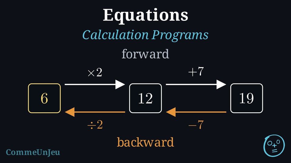
Running the machine forwards gives the output of an input; running it backwards looks for the inputs that give a known output. The gesture is the same from PYP 5 to MYP 5, and only its answers change.

• PYP 5. A machine has the rule “subtract \(3\)”, one of its outputs is \(9\): find the input, then check by running the machine forwards.
• MYP 1. The conversion graph read from the dollars back to the euros runs the machine “multiply by \(1.2\)” backwards, with the rule “divide by \(1.2\)”.
• MYP 2. A calculation program is several small machines in a chain. In this drawing the boxes hold the numbers and each arrow is a machine: $$\boxed{3} \xrightarrow{\times 2} \boxed{6} \xrightarrow{+7} \boxed{13}$$ “When every step can be undone, the program is run backwards with the inverse operations, in the reverse order: from \(13\), subtract \(7\), then divide by \(2\), to find \(3\) again.”
• MYP 5. The preimages of a value: “if the output is known, can the input(s) that produced it be found?” They are read on the graph, then computed: set the formula equal to the output, \(f(x) = y\), and solve the equation. With the square machine, \(9\) has two inputs, \(-3\) and \(3\) (the task taken apart below).
• MYP 5 Extended. The inverse function begins with two machines: the machine “\(-3\)” placed after the machine “\(+3\)” gives back the input. The same lesson warns that not every function has an inverse: each output must come from exactly one input.

Backwards, zero, one or several inputs; the machine is still a function. Running a machine backwards does not always give a function: it is the reason why the square machine, which gives \(16\) to both \(4\) and \(-4\), has no inverse on all the numbers.

“A function is a formula.” The mystery machine, played as “guess my rule”, teaches it. The PYP 4 correction answers: try the rule on all the results, because “One result can suggest a rule; the results can reject a rule, never prove it”. A formula is one way of writing a rule; a table read case by case is another. “A machine that answers the same number to every input is not a function.” In PYP 5, Zoé says a machine that answers \(7\) to every input “doesn't compute anything”. In MYP 5, a table whose outputs are all \(5\) is a function table: “this is the constant function, whose machine answers \(5\) to every question.” “A function may not give the same output twice.” The definition reads in one direction only. On an arrow diagram, the whole test is “one arrow out of every input — the number of arrows arriving at an output does not matter”: 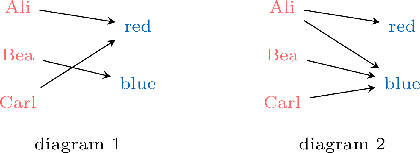Diagram 1 is a function, two pupils sharing red included; diagram 2 is not, Ali sends two arrows. Lina's claim, in MYP 5, is tested on \(x^2\): \(f(-2) = f(2) = 4\), and \(x^2\) is a perfectly good function. “The line between the points was measured.” Sami's exercise in PYP 4: the \(20\,^\circ\)C read halfway between August and September was never measured. The same idea returns with formulas: in MYP 2, the shape of the line between computed points “remains a conjecture”; in MYP 5, joining the points of a table “is a conjecture until the rule gives the values in between”. Image and preimage swapped. The definition of MYP 5 fixes the words on the machine: \(f(x)\) is the image of \(x\), the output; \(x\) is a preimage of \(f(x)\), an input. Ask “which one goes in?” before any calculation. “Two different rules make two different machines.” In PYP 5, Malo's machine “multiply by \(2\)” and Jade's “add the input to itself” give the same output for every input: they are the same function. Two machines are the same when they give the same output to each input, whatever happens inside. The graph read as a picture of the journey. On a distance-time graph, a part that rises is not a hill: the traveller moves away from home. The MYP 1 lesson reads each point as a sentence, and warns that the distance from the start is not the distance travelled. A program undone in the same order. From \(13\), dividing by \(2\) first does not give back \(3\). The MYP 2 definition: the inverse operations, in the reverse order.

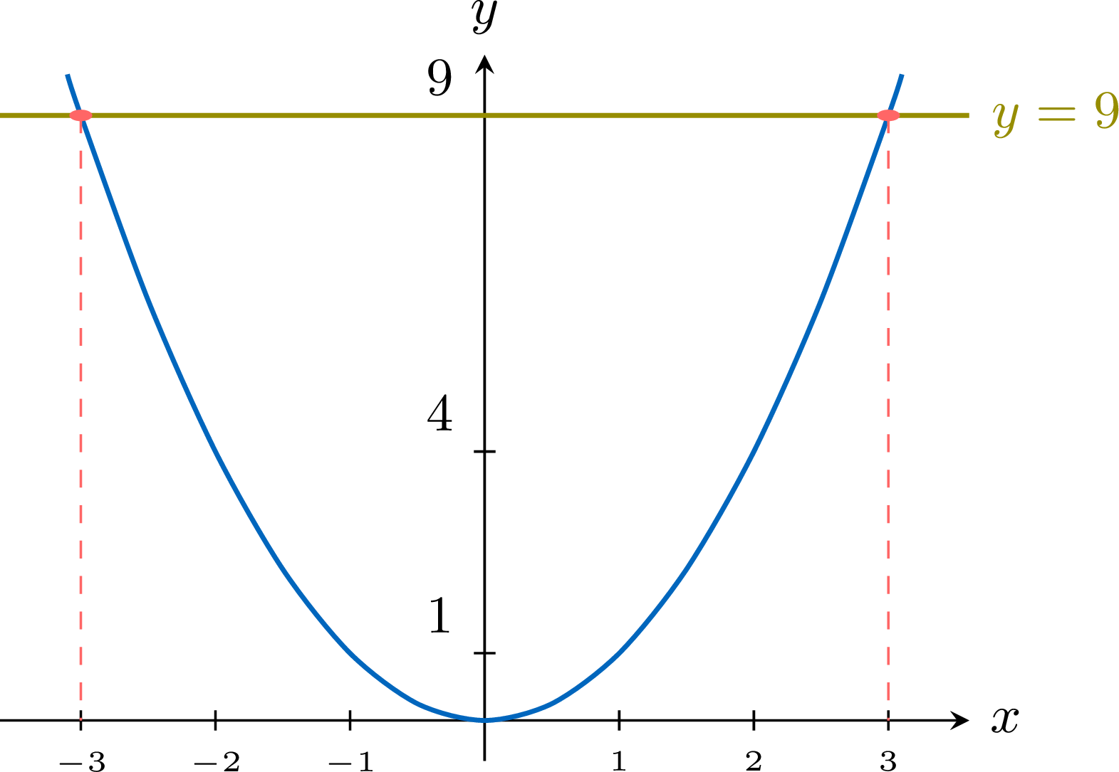
The written exercise of the reasoning group, in MYP 5, asks: the square machine has the rule “square the input”, \(f(x) = x^2\), and accepts every number. Pass \(4\) and \(-4\) through it; run it backwards, to find the inputs that give \(9\), then \(0\), then \(-1\); draw the curve for \(-3 \leq x \leq 3\) and the line \(y = 9\), and read the inputs that give \(9\); decide whether the square machine can be run backwards like the machine “add \(3\)”, with exactly one input for each output. Four settings make it easy or hard.

1. Forwards first. \(4 \longmapsto 16\) and \(-4 \longmapsto 16\): two inputs, one output, which a function allows. The question prepares the next one; let pupils say it before going on.
2. The output. \(9\) has two inputs, \(0\) one, \(-1\) none, “since a square is never negative”: the three cases of the lesson, in one question. The pupil who knows that “the square root of \(9\) is \(3\)” stops at one input.
3. The curve. The line \(y = 9\) meets the curve at two points; below them, on the \(x\)-axis, the inputs \(-3\) and \(3\):
4. The last question. No: backwards, \(9\) would have to give two outputs, \(-3\) and \(3\), so running the machine backwards does not give a function. The square-root machine undoes the square machine only for the inputs that are positive or zero: \(\sqrt{(-3)^2} = 3\), not \(-3\).

What to listen for. The criteria of the correction penalise two answers: only \(3\) for the output \(9\), and “yes, the square root” without the restriction. A third one is worth hearing in class: “it is not a function, since two inputs give \(9\)” — the direction of the definition is still confused; go back to Lina's claim and to the arrow diagrams.

• Draw the machine before writing the rule: the input in red, the rule in olive, the output in blue; then pass a number through it, then write.
• Run it backwards, then check forwards. Every input found backwards is passed again through the machine.
• Play the mystery machine carefully: say “a rule that fits”, test it on every result, accept any output consistent with the rule a pupil found; and show machines given only by a table.
• Show early a machine that answers the same number to every input, and two inputs sharing an output: the constant machine and the square machine are functions.
• Change the drawing with both drawings side by side: the robot and the box, then the box and \(f : x \longmapsto f(x)\). Say it is the same machine.
• Before joining points, ask whether the inputs in between exist, and say that the line between computed points remains a conjecture.
• Write the inputs the machine accepts next to the box, as soon as a rule cannot be applied to every number.
• Keep “relation” for two quantities: the perimeter in terms of the side, with its box and its covariation, \(+1\) cm on the side, \(+4\) cm on the perimeter.

The input-output box was proposed as a “cognitive root” of the function concept by David Tall, Mercedes McGowen and Phil DeMarois (The function machine as a cognitive root for the function concept, PME-NA 22, 2000): a starting point that makes sense to the beginner and keeps its sense later, the tables, formulas and graphs becoming ways of computing what happens between input and output. It is a theoretical paper, and its authors name the limits of their own machine: played as “guess my rule”, it produces the obstacle that every function is given by a formula, hence their advice of everyday machines defined by a procedure, such as the price of sending a letter according to its weight; and the box has no domain drawn on it. In a study of about \(400\) pupils aged \(14\) to \(15\), Zvia Markovits, Bat-Sheva Eylon and Maxim Bruckheimer (Functions today and yesterday, For the Learning of Mathematics, 1986) found three kinds of functions hard to accept: the constant function, the function defined piecewise, the function given only by some points. Shlomo Vinner and Tommy Dreyfus (Images and definitions for the concept of function, Journal for Research in Mathematics Education, 1989) compared the definitions that \(271\) college students and \(36\) junior high school teachers gave with the images of the concept they used: the two often contradict each other, even among those who give the modern definition. Alan Bell and Claude Janvier (The interpretation of graphs representing situations, For the Learning of Mathematics, 1981) report that graphs of situations are misread when their pictorial aspect conflicts with their meaning, and that tables help to study how variables change. Patrick Thompson and Marilyn Carlson (Variation, covariation, and functions, 2017) argue that the view “one input, one output” alone does not equip pupils to reason about two quantities that change together: the course places that covariation in the chapters on relations, with the same box. None of these studies evaluates the progression described in this guide. A research article on these choices is in preparation.