International Baccalaureate · MYP 4
Statistics: Sampling, Spread and Cumulative Frequency
I
Collecting Data
I.1
Types of Variables
Definition — Types of Variables
A variable is a characteristic of an individual in the population that can take different values. Variables are classified into two main types: - Qualitative Variable (Categorical): Represents characteristics that belong to a category or group (e.g., eye colour, type of car, favourite subject).
- Quantitative Variable (Numerical): Represents characteristics that can be counted or measured numerically. These can be further divided into:
- Discrete: The variable can only take specific, separate numerical values (often integers). It is typically data that is counted.
- Continuous: The variable can take any numerical value within a given range. It is typically data that is measured.
Example
We classify some variables from a student survey: - The variable “Favourite Subject” is qualitative.
- The variable “Number of siblings” is a discrete quantitative variable, as the answers can only be integers (0, 1, 2, ...).
- The variable “Height in centimetres” is a continuous quantitative variable, as a student's height could be any value within a range (e.g., 165.2 cm, 165.25 cm, etc.).
Skills to practice
- Sorting Variables into Three Types
I.2
Sampling Methods
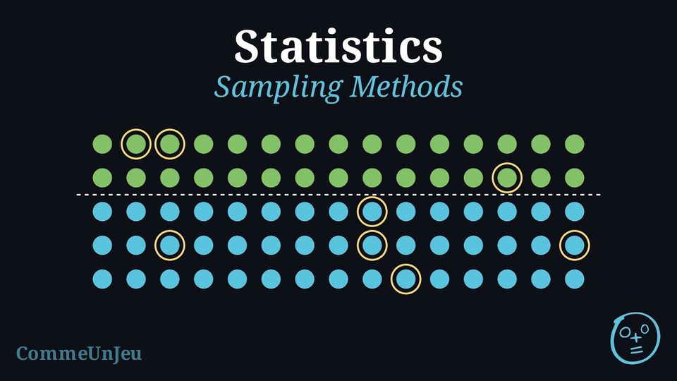
When conducting a survey, our goal is to select a sample that is representative of the entire population. The method used to select this sample is critical. A poorly chosen method can lead to a biased sample, where certain parts of the population are over- or under-represented, making the conclusions invalid.
Definition — Probability Sampling
In probability sampling, every member of the population has a known, non-zero chance of being selected. In these methods, chance — not the surveyor's choices — decides who is selected. - Simple Random Sampling: Every member has an equal chance of selection (more precisely, every possible group of \(n\) individuals has the same chance of being the chosen sample).
Example: Drawing 3 names from a hat containing all 30 students' names. - Systematic Sampling: Members are selected at a regular interval (\(k\)) from an ordered list, starting from a random point between 1 and \(k\).
Example: Surveying every 20th customer entering a store, starting from a randomly chosen one. - Stratified Sampling: The population is divided into subgroups (strata), and a simple random sample is taken from each stratum, often proportional to its size.
Example: A school with 40\(\pourcent\) boys and 60\(\pourcent\) girls takes a random sample of 40 boys and 60 girls.
Definition — Non-Probability Sampling
In non-probability sampling, the selection of the sample is not random and is often based on the researcher's judgement or convenience. These methods are highly prone to bias. - Convenience Sampling: Selecting the most easily accessible members of the population.
Example: Surveying only your own friends about a school-wide issue. - Quota Sampling: Similar to stratified sampling, but individuals within each subgroup are selected non-randomly (e.g., by convenience) until a quota is met.
Example: A researcher needs 30 male and 30 female participants and simply surveys the first 30 of each gender they meet.
Skills to practice
- Identifying Sampling Methods
I.3
Errors in Surveys
Definition — Selection Bias
Selection bias is a systematic error that occurs when the method of selecting a sample causes it to be unrepresentative of the population. Unlike random sampling error, bias pushes the results in a specific direction and does not disappear just by increasing the sample size. Definition — Total Survey Error
The total survey error is the difference between a result calculated from the sample and the true value for the population. It is composed of two types of error: - Sampling Error: Natural, random variation due to observing a sample instead of the whole population.
- Non-Sampling Error: Errors arising from the survey design or execution — selection bias, measurement, recording or non-response errors (they can be systematic or random).
Definition — Measurement Error
Measurement error refers to inaccuracies in the data that arise during the collection process itself. Common causes include: - Poorly worded questions: Ambiguous, “double-barrelled” or leading questions that confuse or influence the respondent.
- Response bias: Respondents provide inaccurate answers due to social desirability (wanting to appear favourable) or misunderstanding the question.
Example
A survey asks students: “Don't you agree that amazing Mathematics is the most important subject for your future?”Identify the source of error.
This is a source of measurement error. The question is leading for two reasons:
- It uses the biased adjective “amazing” to describe mathematics.
- It uses the phrase “Don't you agree”, which pressures the respondent to answer “Yes”.
Definition — Non-Response Error
A non-response error occurs when some of the members chosen for a sample do not answer — they refuse, cannot be reached or do not return the questionnaire — and those who answer differ from those who do not in what the survey measures. The response rate is $$\text{response rate} = \frac{\text{number of members who answered}}{\text{number of members chosen for the sample}},$$ often written as a percentage. A low response rate is a warning: the answers then come from the members who chose to reply, and the results may be biased even when the sample itself was chosen at random. Sending more questionnaires to the same kind of people does not remove this bias. Example
An online shop emails a satisfaction questionnaire to \(800\) customers chosen at random; \(248\) of them reply.Calculate the response rate, and explain why the results may be biased even though the \(800\) customers were chosen at random.
$$\text{response rate} = \frac{248}{800} = 0.31 = 31\pourcent.$$ More than two customers out of three did not reply. Customers who reply to a satisfaction questionnaire are often those with a strong opinion, very satisfied or very dissatisfied, so the \(248\) replies may not represent the \(800\) customers chosen, and even less all the customers of the shop. The random choice of the \(800\) protects against selection bias, not against non-response error. Reminders or a shorter questionnaire can raise the response rate, and contacting again a random part of the non-respondents gives an idea of whether they answer differently.
Skills to practice
- Evaluating Samples and Response Rates
II
Centre and Spread
II.1
Quartiles and the Interquartile Range
Definition — Quartiles and IQR
Quartiles are values that divide an ordered dataset into four parts, each holding about a quarter of the values. - The lower quartile (Q1) is the median of the lower half of the data.
- The median (Q2) is the overall median of the data.
- The upper quartile (Q3) is the median of the upper half of the data.
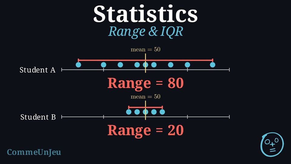
The interquartile range (IQR) is the range of the middle 50\(\pourcent\) of the data. It is less affected by extreme outliers than the range. $$ \text{IQR} = Q_3 - Q_1 $$
Example
Find the quartiles and the interquartile range for the data: \(1, 19, 10, 2, 18, 10, 5, 15, 10\). - Order the data: \(1, 2, 5, 10, 10, 10, 15, 18, 19\).
- Find the median (Q2): The middle value is the 5th one, so \(Q_2 = 10\). $$ 1, 2, 5, 10, \underline{10}, 10, 15, 18, 19 $$
- Split the data into two halves (excluding Q2): Lower half: \(1, 2, 5, 10\) \(\quad\) Upper half: \(10, 15, 18, 19\).
- Find the lower quartile (Q1): Find the median of the lower half. $$ 1, \underline{2, 5}, 10 \rightarrow Q_1 = \frac{2+5}{2} = 3.5 $$
- Find the upper quartile (Q3): Find the median of the upper half. $$ 10, \underline{15, 18}, 19 \rightarrow Q_3 = \frac{15+18}{2} = 16.5 $$
- Calculate the IQR: $$ \text{IQR} = Q_3 - Q_1 = 16.5 - 3.5 = 13 $$
Definition — Interquartile Range
The interquartile range (IQR) of a dataset is the difference between its quartiles: $$\text{IQR} = Q_3 - Q_1.$$ It is the width of the zone holding at least the central half of the values. Unlike the range, which is read off the two end values, it is read off positions in the ordered list: making the smallest value even smaller, or the largest even larger, does not change it — unless a half of the data holds so few values that this value enters the calculation of a quartile.
Two Conventions for Quartiles
Two conventions coexist for quartiles. In one convention, the quartiles are the medians of the two halves of the dataset (they may fall between two values). In the other, used in the following definition, the quartiles are always values of the dataset. The two conventions can give different numbers on the same dataset — what matters is to state which convention is used.
Definition — Quartiles as Values of the Dataset
For an ordered dataset of \(N\) values: - the first quartile \(Q_1\) is the smallest value of the dataset such that at least one quarter (\(25\pourcent\)) of the values are less than or equal to it;
- the third quartile \(Q_3\) is the smallest value of the dataset such that at least three quarters (\(75\pourcent\)) of the values are less than or equal to it.
Skills to practice
- Finding the Interquartile Range with the Medians of the Halves
- Finding the Interquartile Range of Ordered Data
II.2
The Linearity of the Mean
Proposition — Linearity of the Mean
Take a dataset \(x_1, x_2, \ldots, x_n\) with mean \(\bar{x}\), and two numbers \(a\) and \(b\). If every value is replaced by \(y_i = a x_i + b\), then the new mean is $$\bar{y} = a\,\bar{x} + b.$$ The mean follows the transformation: there is no need to know the individual values to update it.
$$\begin{aligned}[t] \bar{y} &= \frac{y_1 + y_2 + \cdots + y_n}{n} \\
&= \frac{(a x_1 + b) + (a x_2 + b) + \cdots + (a x_n + b)}{n} \\
&= \frac{a(x_1 + x_2 + \cdots + x_n) + n\,b}{n} && \text{(grouping the \(a x_i\) and the \(n\) copies of \(b\))}\\
&= a\,\frac{x_1 + x_2 + \cdots + x_n}{n} + b \\
&= a\,\bar{x} + b. \end{aligned}$$
Example
The mean price of the items in a shop is \(\bar{x} = \dollar 20\). Every price is doubled, then reduced by \(\dollar 3\). Find the new mean price.
Every price is replaced by \(y_i = 2 x_i - 3\), so by linearity $$\begin{aligned}[t] \bar{y} &= 2\,\bar{x} - 3 \\
&= 2 \times 20 - 3 \\
&= 37. \end{aligned}$$ The new mean price is \(\dollar 37\).
Check on a tiny dataset: prices \(\dollar 10\) and \(\dollar 30\) have mean \(\dollar 20\); the new prices \(\dollar 17\) and \(\dollar 57\) have mean \(\frac{17+57}{2} = \dollar 37\).
Check on a tiny dataset: prices \(\dollar 10\) and \(\dollar 30\) have mean \(\dollar 20\); the new prices \(\dollar 17\) and \(\dollar 57\) have mean \(\frac{17+57}{2} = \dollar 37\).
Skills to practice
- Updating a Mean without the Data
II.3
Adding or Removing a Value
Proposition — Adding or Removing a Value
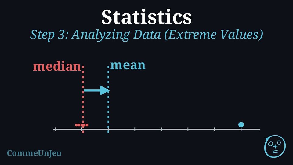
Let a series of \(n\) values have mean \(m\). - Adding a value \(x\) gives a series of \(n + 1\) values whose mean is $$m' = \frac{n\,m + x}{n + 1}, \qquad\text{and}\qquad m' - m = \frac{x - m}{n + 1}.$$ The mean moves towards the added value: it increases if \(x > m\), decreases if \(x < m\), and does not change if \(x = m\). The move is a fraction \(\dfrac{1}{n + 1}\) of the gap \(x - m\): for a given gap, the larger the series, the smaller the move.
- Removing a value \(x\) (\(n \geq 2\)) gives a series of \(n - 1\) values whose mean is $$m' = \frac{n\,m - x}{n - 1}, \qquad\text{and}\qquad m' - m = \frac{m - x}{n - 1}.$$ The mean moves away from the removed value: it increases if \(x < m\), decreases if \(x > m\), and does not change if \(x = m\).
- The median is read on the ordered list, at the middle position; adding or removing one value moves the middle by half a position. When the number of values was odd, the median was the middle value: the new median is the mean of the old median and the value next to it, below or above, in the new ordered list (removing the median itself leaves the mean of its two neighbours). When the number of values was even, the median was the mean of the two middle values: the new median is one of these two values, or the added value itself when it falls between them. In both cases, once the added or removed value lies beyond the values around the middle (an extreme value, for instance), its exact size plays no role.
The sum of the \(n\) values is \(n\,m\) (definition of the mean). After adding \(x\), the sum is \(n\,m + x\) and there are \(n + 1\) values, so \(m' = \dfrac{n\,m + x}{n + 1}\). Then $$m' - m = \frac{n\,m + x}{n + 1} - \frac{(n + 1)\,m}{n + 1} = \frac{n\,m + x - n\,m - m}{n + 1} = \frac{x - m}{n + 1},$$ which has the sign of \(x - m\). After removing \(x\) instead, the sum is \(n\,m - x\) over \(n - 1\) values, so \(m' = \dfrac{n\,m - x}{n - 1}\) and $$m' - m = \frac{n\,m - x - (n - 1)\,m}{n - 1} = \frac{m - x}{n - 1},$$ which has the sign of \(m - x\). For the median: in the ordered list of \(n + 1\) values, every value keeps its rank except those beyond the inserted value, which move by one rank. If \(n\) is odd, the old median remains one of the two central values (it keeps its rank when \(x\) is above it, and moves by one rank when \(x\) is below it), and the new median is the average of it and its neighbour on the side of \(x\) (or of it and \(x\), when \(x\) falls between them): at most half the gap. If \(n\) is even, the new median is the value at the middle rank: one of the two old middle values, or \(x\) itself when \(x\) lies between them. Removing a value works the same way, the ranks beyond the removed value moving by one in the other direction.
Example
The marks of five pupils at a test are \(8\), \(10\), \(11\), \(12\), \(14\). - Compute the mean and the median.
- A sixth mark, \(20\), is added. Compute the new mean and the new median; which measure moved the most?
- Starting again from the five marks, the mark \(14\) is removed. Compute the new mean and the new median.
- Starting from the six marks \(8\), \(10\), \(11\), \(12\), \(14\), \(20\), a seventh mark, \(11.8\), is added. Compute the new median.
- Sum \(8 + 10 + 11 + 12 + 14 = 55\), so \(m = \dfrac{55}{5} = 11\). The list is ordered and \(n = 5\) is odd: the median is the third value, \(11\).
- New mean: \(m' = \dfrac{5 \times 11 + 20}{6} = \dfrac{75}{6} = 12.5\); indeed \(m' - m = \dfrac{20 - 11}{6} = 1.5\). New median: the ordered list \(8, 10, 11, 12, 14, 20\) has six values, the median is \(\dfrac{11 + 12}{2} = 11.5\). The mean moved by \(1.5\), the median by \(0.5\) only: the added value pulls the mean, while the median just steps halfway to its neighbour.
- Removing \(14\): \(m' = \dfrac{5 \times 11 - 14}{4} = \dfrac{41}{4} = 10.25\) (the mean moves away from \(14\), downwards). Ordered list \(8, 10, 11, 12\): median \(\dfrac{10 + 11}{2} = 10.5\).
- The six marks have median \(11.5\), between the middle values \(11\) and \(12\). The ordered list of seven marks is $$8,\ 10,\ 11,\ 11.8,\ 12,\ 14,\ 20$$ and the median is the fourth value, \(11.8\): the added mark fell between the two middle values and became the median itself — still between \(11\) and \(12\), as the lesson says.
Skills to practice
- Calculating the New Mean and Median
III
Grouped Data
III.1
Histograms
The \(40\) pupils of a class noted how long, in minutes, their journey to school takes. The times were grouped:
In a bar chart, the bars stand apart, one per category. Here the times run on without a break from \(0\) to \(40\) minutes. How can a chart show that each group covers a whole interval of times?
| Time (min) | Number of pupils |
| \(0 \le t < 10\) | \(12\) |
| \(10 \le t < 20\) | \(16\) |
| \(20 \le t < 30\) | \(8\) |
| \(30 \le t < 40\) | \(4\) |
By rectangles that touch, drawn over a numbered axis: each rectangle stands on its whole interval, and its height gives the number of pupils. The four rectangles fill the axis from \(0\) to \(40\) without a gap, just as the times do. Such a chart is a histogram. 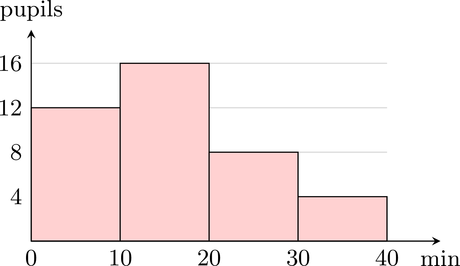
Definition — Classes and Histogram
When a quantity takes many different values (a time, a height, a mass…), the values are grouped into classes: intervals, here all of the same width, such as \(0 \le t < 10\) — from \(0\) included to \(10\) excluded, so that each value belongs to exactly one class. The frequency of a class is the number of values it contains. A histogram represents such a series: along a numbered horizontal axis, each class is drawn as a rectangle whose base is the class and whose height is its frequency. The rectangles touch, since the classes follow each other. Method — Drawing a Histogram
- Mark the horizontal axis with the bounds of the classes, evenly spaced, since the classes have the same width.
- Mark the vertical axis with the frequencies, from \(0\).
- Draw one rectangle per class: its base is the class, its height the frequency; the rectangles touch.
- Name the two axes, with their units.
Example
The masses of \(50\) apples picked in an orchard were grouped: | Mass (g) | Frequency |
| \(100 \le m < 120\) | \(6\) |
| \(120 \le m < 140\) | \(14\) |
| \(140 \le m < 160\) | \(18\) |
| \(160 \le m < 180\) | \(9\) |
| \(180 \le m < 200\) | \(3\) |
- Draw the histogram of this series.
- How many apples weigh at least \(140\) g? What percentage of the apples is that?
- The five classes have the same width, \(20\) g: the axis is marked from \(100\) to \(200\) in steps of \(20\), and each rectangle has the height of its frequency.
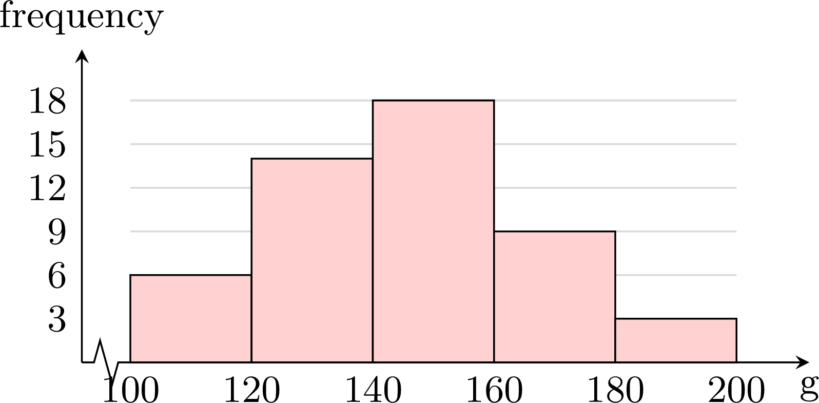
- The apples of at least \(140\) g are those of the last three classes: \(18 + 9 + 3 = 30\) apples, that is \(\dfrac{30}{50} = 0.6 = 60~\pourcent\) of the apples.
Example
The histogram shows the ages of the members of a sports club. 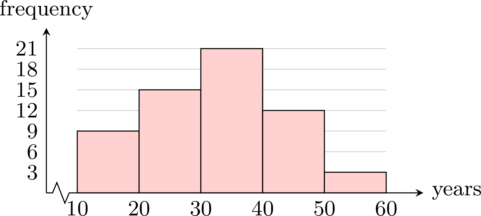
- What is the frequency of the class \(30 \le a < 40\)? How many members does the club have?
- What is the relative frequency of the members under \(30\)? Give it as a decimal, then as a percentage.
- What can be said about the range of the ages?
- The rectangle over \(30 \le a < 40\) rises to \(21\): \(21\) members. In total: \(9 + 15 + 21 + 12 + 3 = 60\) members.
- Under \(30\): the first two classes, \(9 + 15 = 24\) members out of \(60\). Relative frequency: \(\dfrac{24}{60} = 0.4\), that is \(40~\pourcent\).
- The exact ages are not known, only their classes: the youngest member is at least \(10\), the oldest under \(60\). The range is therefore less than \(60 - 10 = 50\) years — grouping the values hides its exact value.
Bar Chart or Histogram?
A bar chart shows separate categories or isolated values: its bars stand apart. A histogram shows classes that follow each other: its rectangles touch. With classes of the same width, the height of a rectangle reads directly as the frequency of its class.
Skills to practice
- Reading a Histogram
- Drawing and Using a Histogram
III.2
Estimating the Mean of Grouped Data
Method — Estimating the Mean of Grouped Data
The exact values inside a class are unknown, so the mean is estimated by representing each class by its midpoint (the centre of the interval). - Find each class midpoint \(m_i\): the average of the two endpoints of the class.
- Multiply each midpoint by the class frequency \(n_i\) to get \(n_i m_i\).
- Estimate the mean as a weighted mean of the midpoints: $$ \bar{x} \approx \frac{\sum n_i m_i}{N}, \qquad N = \sum n_i . $$
Example
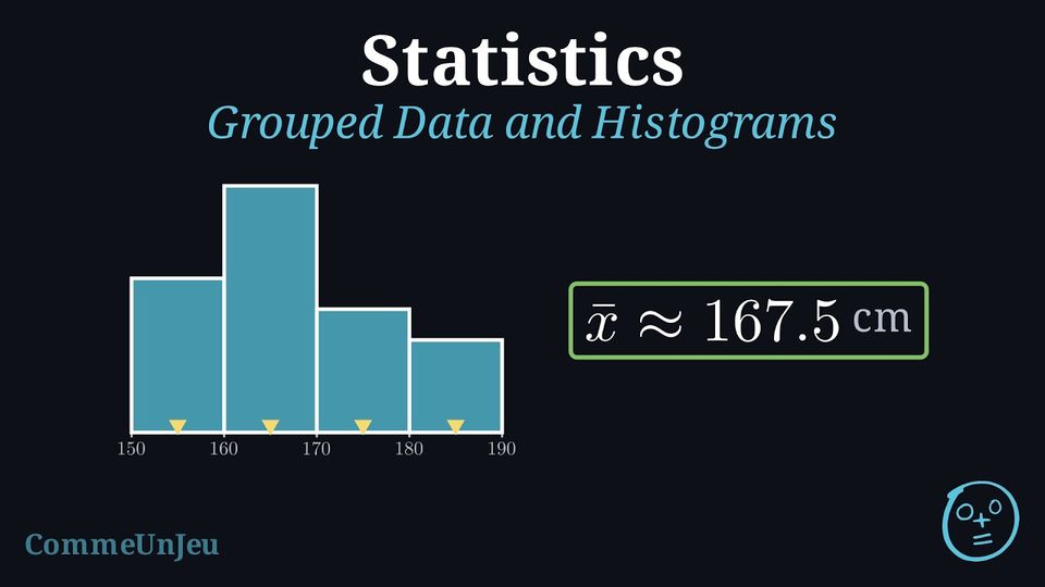
The heights (in cm) of \(20\) students were measured and grouped into classes. Draw the histogram and estimate the mean height. | Height (cm) | \([150,160)\) | \([160,170)\) | \([170,180)\) | \([180,190)\) | Total |
| Frequency \(n_i\) | 5 | 8 | 4 | 3 | 20 |
Histogram. The bars are adjacent (no gaps), since the classes are consecutive intervals. 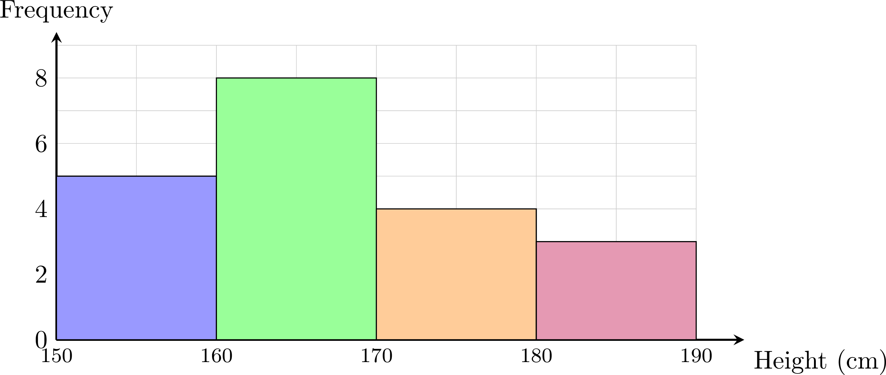
Estimated mean. The midpoints are \(m_i = 155, 165, 175, 185\).
$$ \begin{aligned} \bar{x} &\approx \frac{\sum n_i m_i}{N} &&\text{(midpoint estimate)} \\
&= \frac{155\times 5 + 165\times 8 + 175\times 4 + 185\times 3}{20} &&\text{(substitute)} \\
&= \frac{3350}{20} &&\text{(add)} \\
&= 167.5 . &&\text{(divide)} \end{aligned} $$ The estimated mean height is about \(167.5\) cm.
| Class | \([150,160)\) | \([160,170)\) | \([170,180)\) | \([180,190)\) | Total |
| Midpoint \(m_i\) | 155 | 165 | 175 | 185 | |
| \(n_i\) | 5 | 8 | 4 | 3 | 20 |
| \(n_i m_i\) | 775 | 1320 | 700 | 555 | 3350 |
Proposition — Mean from the Class Means
A series of \(N\) values is sorted into \(k\) classes of frequencies \(n_1, n_2, \ldots, n_k\), and the mean of the values of each class is known: \(\bar{x}_1, \bar{x}_2, \ldots, \bar{x}_k\). The mean of the whole series is the weighted mean of the class means, each mean weighted by the frequency of its class: $$\textcolor{colorprop}{\bar{x} = \frac{n_1 \bar{x}_1 + n_2 \bar{x}_2 + \cdots + n_k \bar{x}_k}{N}}, \qquad N = n_1 + n_2 + \cdots + n_k.$$ Special case: when the values of a class are assumed to be spread uniformly between its bounds — the model behind the midpoint estimate — the mean of the class is taken to be its midpoint, and the formula gives the estimate of the mean by the midpoints.
By the definition of the mean, the sum of the \(n_i\) values of the class number \(i\) is \(n_i \bar{x}_i\). The sum of all \(N\) values is the sum of these class sums, so $$\begin{aligned} \bar{x} &= \frac{\text{sum of the } N \text{ values}}{N} && \text{(definition of the mean)} \\
&= \frac{n_1 \bar{x}_1 + n_2 \bar{x}_2 + \cdots + n_k \bar{x}_k}{N}. && \text{(sum class by class)} \end{aligned}$$ When the values of a class are modelled as spread uniformly between its two bounds, they are balanced around the midpoint of the class, which is then taken as the mean of the class: the formula becomes the midpoint estimate.
Example
The monthly salaries (in dollars) of the \(40\) employees of a company are grouped into three classes of equal width. The payroll also gives the mean salary of each class. | Salary | \([1000, 1500)\) | \([1500, 2000)\) | \([2000, 2500)\) |
| Frequency \(n_i\) | \(12\) | \(20\) | \(8\) |
| Mean of the class \(\bar{x}_i\) | \(1320\) | \(1700\) | \(2300\) |
- Compute the mean salary of the company.
- Compare it with the estimate by the midpoints of the classes.
- The mean of the series is the weighted mean of the class means: $$\begin{aligned} \bar{x} &= \frac{n_1 \bar{x}_1 + n_2 \bar{x}_2 + n_3 \bar{x}_3}{N} && \text{(Proposition ``Mean from the Class Means'')} \\ &= \frac{12 \times 1320 + 20 \times 1700 + 8 \times 2300}{40} && \text{(substitute)} \\ &= \frac{15\,840 + 34\,000 + 18\,400}{40} = \frac{68\,240}{40} && \text{(multiply, add)} \\ &= 1706. \end{aligned}$$ The mean salary is \(\dollar 1706\). It is exact, since the mean of each class is known.
- The midpoints are \(1250\), \(1750\) and \(2250\); the estimate is \(\dfrac{12 \times 1250 + 20 \times 1750 + 8 \times 2250}{40} = \dfrac{68\,000}{40} = 1700\), that is \(\dollar 1700\). The estimate is \(\dollar 6\) below the true mean. Class by class, the midpoint replaces the true mean: it is too low in the first and last classes (\(1250\) for \(1320\), \(2250\) for \(2300\)) and too high in the middle one (\(1750\) for \(1700\)), and the balance, weighted by the frequencies, is \(\dfrac{12 \times (-70) + 20 \times 50 + 8 \times (-50)}{40} = \dfrac{-240}{40} = -6\), the gap of \(\dollar 6\). The midpoint estimate is exact when the values are spread uniformly in each class; otherwise it can be off in either direction, and the mean from the class means is the value to report.
Skills to practice
- Estimating a Mean from Grouped Data
III.3
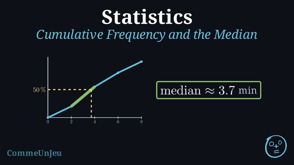
Cumulative Frequency Curves and the Median Class
Definition — Cumulative Frequency
In a frequency table, the cumulative frequency of a value is the number of data points less than or equal to that value. It is obtained by adding the frequencies from the smallest value up to that value; the last cumulative frequency is the total number \(N\) of data points. Definition — Cumulative-Frequency Curve (Ogive)
When data is grouped into classes, the running totals can be displayed graphically as the cumulative-frequency curve (or ogive). It is built by plotting each cumulative frequency against the upper boundary of its class and joining the points in order by straight segments, starting from the lower boundary of the first class at height \(0\). The curve never goes down: it climbs from \(0\) to the total \(N\), and the number of values below any level can be estimated from it. In particular, the median is estimated by reading across from the height \(\dfrac{N}{2}\) on the vertical axis to the curve, then down to the horizontal axis. In the same way, the lower quartile \(Q_1\) and the upper quartile \(Q_3\) are estimated by reading across from the heights \(\dfrac{N}{4}\) and \(\dfrac{3N}{4}\), which gives an estimate of the interquartile range \(Q_3 - Q_1\). Example
The table gives the test scores (out of \(100\)) of \(50\) students, grouped into classes. Draw the cumulative-frequency curve and use it to estimate the median score. | Score | \([0,20)\) | \([20,40)\) | \([40,60)\) | \([60,80)\) | \([80,100)\) | Total |
| Frequency \(n_i\) | 5 | 10 | 20 | 10 | 5 | 50 |
Form the cumulative frequencies, taking each one at the upper boundary of its class:
Plotting these points (with \((0,0)\)) and joining them gives the ogive: 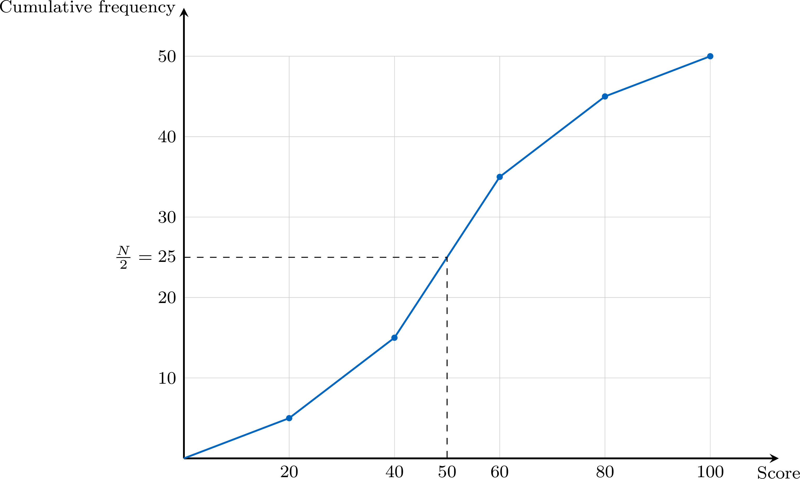
With \(N = 50\), read across from \(\dfrac{N}{2} = 25\) to the curve and down to the axis: the curve reaches this height at a score of about \(50\), so $$ \text{median} \approx 50 \text{ marks.} $$
| Upper boundary | 20 | 40 | 60 | 80 | 100 |
| Cumulative frequency | 5 | 15 | 35 | 45 | 50 |
Definition — Median Class
For a series of \(N\) values grouped into classes, the median class is the class where the median is located: reading the cumulative frequencies in order, it is the first class whose cumulative frequency reaches or exceeds \(\dfrac{N}{2}\). Equivalently, it is the first class whose cumulative relative frequency reaches or exceeds \(50\pourcent\). If a cumulative frequency is exactly \(\dfrac{N}{2}\), the middle of the series falls on the boundary between that class and the next one, and the estimate below returns that boundary. Method — Estimating the Median by a Uniform Spread in the Median Class
The exact values inside the median class are unknown. Assuming that its \(n_c\) values are spread uniformly between its bounds \(a\) and \(b\): - Compute the cumulative frequencies and find the median class \([a, b)\); write \(n_{\text{before}}\) for the cumulative frequency of the classes before it.
- Count the values needed inside the median class to reach the middle: \(\dfrac{N}{2} - n_{\text{before}}\), out of the \(n_c\) values of the class.
- Move along the class in the same proportion: $$\text{median} \approx a + \frac{\dfrac{N}{2} - n_{\text{before}}}{n_c} \times (b - a).$$
Cumulative Frequency Polygon
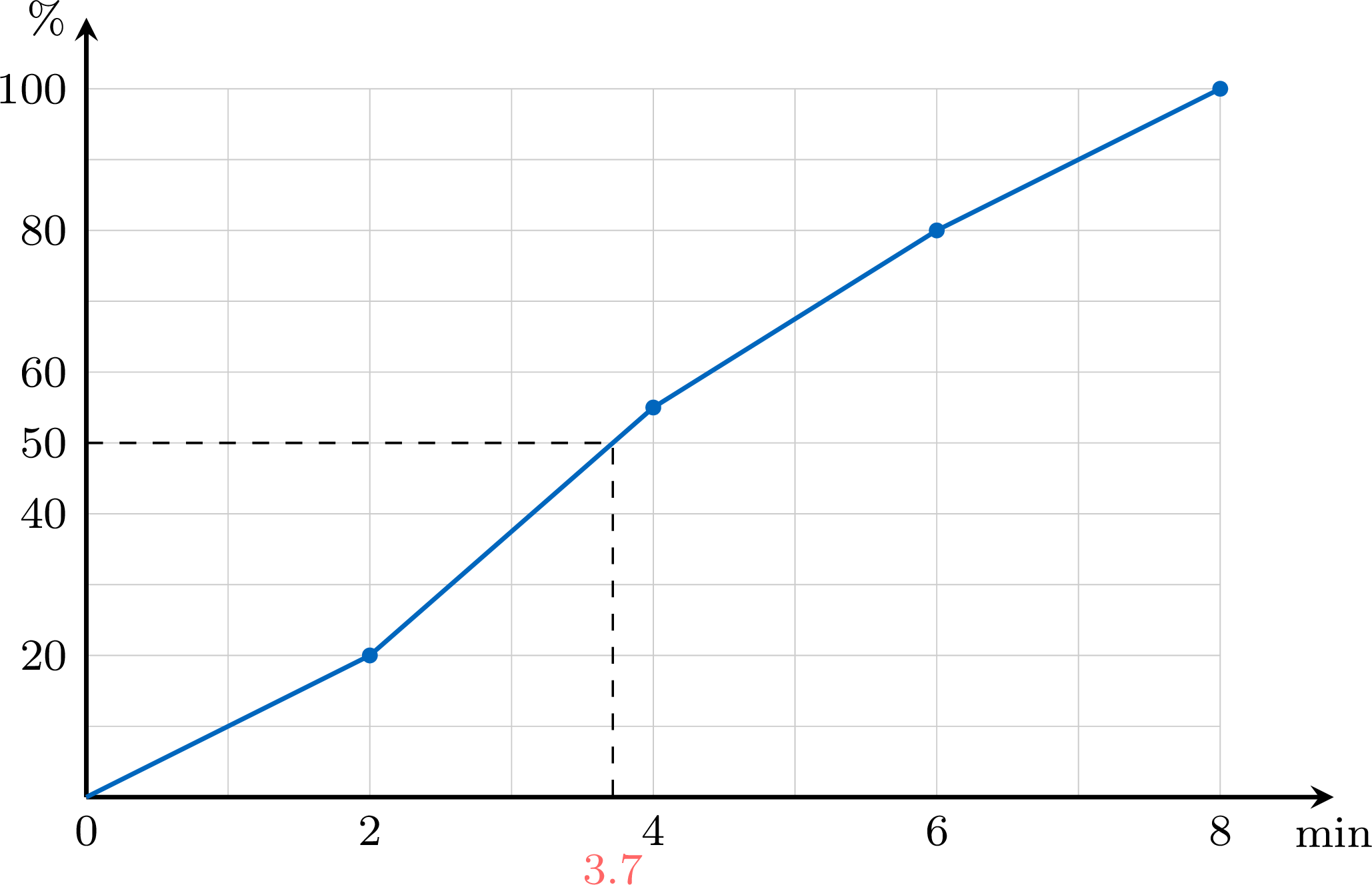
Dividing each cumulative frequency by \(N\) gives the cumulative relative frequencies, which run from \(0\) to \(1\), that is from \(0\pourcent\) to \(100\pourcent\). Plotted against the upper bounds of the classes and joined by segments from the lower bound of the first class, they form the cumulative frequency polygon: the same broken line as the cumulative-frequency curve, with a vertical axis in percentages. An estimate of the median is read at the height \(50\pourcent\); the proportion of the values below a class boundary is read directly on the vertical axis, and between two boundaries the polygon gives an estimate of it, whatever the size \(N\) of the series — which makes the polygon the right tool to compare two series of different sizes.
Example
The durations (in minutes) of \(80\) phone calls received by a help desk are grouped into classes of equal width. | Duration | \([0, 2)\) | \([2, 4)\) | \([4, 6)\) | \([6, 8)\) |
| Frequency \(n_i\) | \(16\) | \(28\) | \(20\) | \(16\) |
- Determine the median class.
- Estimate the median duration, assuming a uniform spread in the median class.
- Draw the cumulative frequency polygon and check the estimate on it.
- The cumulative frequencies, taken at the upper bounds, are \(16\), \(44\), \(64\), \(80\). With \(N = 80\), the middle is \(\dfrac{N}{2} = 40\): the first cumulative frequency to reach \(40\) is \(44\), at the class \([2, 4)\). The median class is \([2, 4)\).
- Before the median class, \(n_{\text{before}} = 16\) calls; the class holds \(n_c = 28\) calls between \(a = 2\) and \(b = 4\). $$\begin{aligned} \text{median} &\approx a + \frac{\dfrac{N}{2} - n_{\text{before}}}{n_c} \times (b - a) && \text{(uniform spread in the median class)} \\ &= 2 + \frac{40 - 16}{28} \times 2 && \text{(substitute)} \\ &= 2 + \frac{24}{28} \times 2 = 2 + \frac{12}{7} && \text{(simplify)} \\ &\approx 3.7 \text{ min.} \end{aligned}$$
- The cumulative relative frequencies are \(\dfrac{16}{80} = 20\pourcent\), \(\dfrac{44}{80} = 55\pourcent\), \(\dfrac{64}{80} = 80\pourcent\) and \(100\pourcent\).
Skills to practice
- Reading Cumulative Frequencies of Grouped Data
- Using Cumulative Frequency Curves
IV
Going further
Skills to practice
- Solving Problems with Grouped Data
- Solving Problems with Histograms
- Investigating Patterns in Measures of Centre and Spread
- Quiz
Jump to section