International Baccalaureate · DP 2: Applications and Interpretation HL
Discrete Random Variables
I
Random Variables
I.1
Random Variables and Their Values
From Events to Numbers
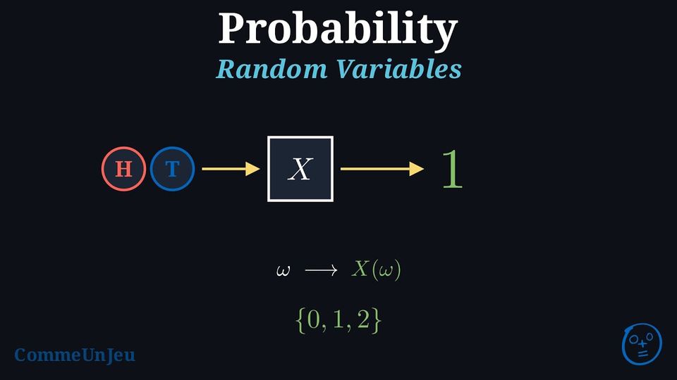
An event is a set of outcomes and its probability a number. Many questions about a random experiment are about a number attached to each outcome rather than about an event: the gain in a game, the number of heads in three tosses, the sum of two dice. Such a number is not fixed in advance, it depends on the outcome that chance produces; it is what the next definition sets down under the name of random variable.
Definition — Random Variable
A random variable, denoted \(X\), is a function that assigns a numerical value to each outcome \(\omega\) of the sample space \(U\) (also written \(\Omega\)). We write this value as \(X(\omega)\). 
Example
Let \(X\) be the number of heads when tossing 2 fair coins:  (red coin) and
 (blue coin). Find \(X(\textcolor{colordef}{H},\textcolor{colorprop}{T})\).
The outcome \((\textcolor{colordef}{H},\textcolor{colorprop}{T})\) means the red coin shows heads (H) and the blue coin shows tails (T). Since \(X\) counts heads, there’s 1 head. Thus, \(X(\textcolor{colordef}{H},\textcolor{colorprop}{T}) = 1\).
Definition — Discrete Random Variable
A random variable is discrete if its set of possible values is finite or countably infinite. This means we can list all possible values. Unless stated otherwise, the random variables considered take finitely many values; the rank of a first success, met later, is the exception. Definition — Events Involving a Random Variable
For a random variable \(X\): - \((X = x)\): The set of outcomes where \(X\) takes the value \(x\).
- \((X \leq x)\): The set of outcomes where \(X\) is less than or equal to \(x\).
- \((X \geq x)\): The set of outcomes where \(X\) is greater than or equal to \(x\).
Example
Let \(X\) be the number of heads when tossing 2 coins: and . List the outcomes for \((X = 0)\), \((X = 1)\), \((X = 2)\), \((X \leq 1)\), and \((X \geq 1)\). - \((X = 0) = \{(\textcolor{colordef}{T},\textcolor{colorprop}{T})\}\) (no heads).
- \((X = 1) = \{(\textcolor{colordef}{T},\textcolor{colorprop}{H}), (\textcolor{colordef}{H},\textcolor{colorprop}{T})\}\) (one head).
- \((X = 2) = \{(\textcolor{colordef}{H},\textcolor{colorprop}{H})\}\) (two heads).
- \((X \leq 1) = (X = 0) \cup (X = 1) = \{(\textcolor{colordef}{T},\textcolor{colorprop}{T}), (\textcolor{colordef}{T},\textcolor{colorprop}{H}), (\textcolor{colordef}{H},\textcolor{colorprop}{T})\}\) (at most one head).
- \((X \geq 1) = (X = 1) \cup (X = 2) = \{(\textcolor{colordef}{T},\textcolor{colorprop}{H}), (\textcolor{colordef}{H},\textcolor{colorprop}{T}), (\textcolor{colordef}{H},\textcolor{colorprop}{H})\}\) (at least one head).
Example
A quiz has three questions, each with four options and one correct answer. A student answers each question at random, independently of the others. Define a random variable that models the situation, give its possible values, and compute the probability that the student gets every answer wrong. - The variable: let \(X\) be the number of correct answers among the three. To each outcome, a sequence of three chosen options, \(X\) attaches the count of correct ones.
- Its possible values: \(0\), \(1\), \(2\) and \(3\).
- The event \((X = 0)\) is “the three answers are wrong”, and each answer is wrong with probability \(\frac{3}{4}\): $$\begin{aligned}[t] P(X = 0) &= \frac{3}{4} \times \frac{3}{4} \times \frac{3}{4} && \scriptscriptstyle\text{(independent answers)} \\ &= \frac{27}{64} \approx 0.42. \end{aligned}$$
Skills to practice
- Finding Events Involving a Random Variable
I.2
Probability Distributions
Forgetting the Outcomes and Keeping the Values
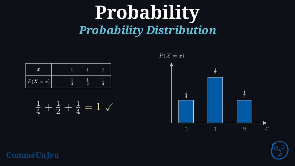
Once the variable is defined, one often sets the outcomes aside and keeps only what \(X\) produces: its values, each with the probability of the event “\(X\) takes this value”. Recording these probabilities, as a table or as a formula, is what the next definition calls the probability distribution of \(X\). The outcomes come back whenever such a probability has to be computed.
Definition — Probability Distribution
The probability distribution of a random variable \(X\) lists the probability \(P(X = x_i)\) for each possible value \(x_1,x_2,\dots,x_n\). Here each \(x_i\) is a possible value of \(X\) — a real number — not an outcome. It can be shown as a table or formula. Proposition — Characteristic of a Probability Distribution
For a random variable \(X\) with possible values \(x_1,x_2,\dots,x_n\), we have - \(0 \leq P(X=x_i) \leq 1\) for all \(i=1,\dots,n\),
- \(\displaystyle\sum_{i=1}^n P(X=x_i) =P(X=x_1)+P(X=x_2)+\dots+P(X=x_n)= 1 \).
Example
Let \(X\) be the number of heads when tossing, independently, 2 fair coins: and . - List the possible values of \(X\).
- Find the probability distribution.
- Create the probability table.
- Draw the probability distribution graph.
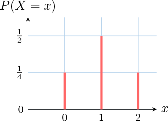
- Possible values: \(0\) (no heads), \(1\) (one head), \(2\) (two heads).
- Probability distribution:
- \(P(X = 0) = P(\{(\textcolor{colordef}{T},\textcolor{colorprop}{T})\}) = \frac{1}{4}\),
- \(P(X = 1) = P(\{(\textcolor{colordef}{T},\textcolor{colorprop}{H}), (\textcolor{colordef}{H},\textcolor{colorprop}{T})\}) = \frac{2}{4} = \frac{1}{2}\),
- \(P(X = 2) = P(\{(\textcolor{colordef}{H},\textcolor{colorprop}{H})\}) = \frac{1}{4}\).
- Probability table:
\(x\) 0 1 2 \(P(X = x)\) \(\frac{1}{4}\) \(\frac{1}{2}\) \(\frac{1}{4}\) - Graph:
Skills to practice
- Finding a Probability Distribution
II
Expected Value and Variance
II.1
Expected Value
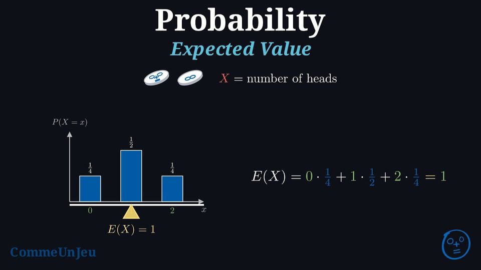
The expected value of a random variable \(X\) is the "average you’d expect if you repeated the experiment many times". It’s found by taking all possible values, multiplying each by its probability, and adding them up — essentially a weighted average where the probabilities act as the weights.
Definition — Expected Value
For a random variable \(X\) with possible values \(x_1, x_2, \ldots, x_n\), the expected value, \(E(X)\), also called the mean, is:$$\begin{aligned}E(X) &= \sum_{i=1}^{n} x_i P(X = x_i)\\
&= x_1 P(X = x_1) + x_2 P(X = x_2) + \cdots + x_n P(X = x_n)\\
\end{aligned}$$ Example
You toss 2 fair coins, and \(X\) is the number of heads. The probability distribution is: | \(x\) | 0 | 1 | 2 |
| \(P(X = x)\) | \(\frac{1}{4}\) | \(\frac{1}{2}\) | \(\frac{1}{4}\) |
Calculate \(E(X)\) using the formula:$$\begin{aligned}E(X) &= 0 \times \frac{1}{4} + 1 \times \frac{1}{2} + 2 \times \frac{1}{4} \\
&= \frac{1}{2} + \frac{2}{4} \\
&= 1\end{aligned}$$ So, on average, you expect 1 head when tossing 2 coins.
Proposition — Expectation of \(aX + b\)
For any random variable \(X\) and constants \(a\) and \(b\), the expected value of a linear transformation of \(X\) is:$$ E(aX + b) = aE(X) + b $$ This property is derived from two simpler rules: - \(E(aX) = aE(X)\) (The expectation of a scaled variable is the scaled expectation).
- \(E(X+b) = E(X) + b\) (The expectation of a shifted variable is the shifted expectation).
Let \(x_1, \ldots, x_n\) be the values of \(X\).
- Case \(a = 0\). The variable \(aX + b\) is the constant \(b\): it takes the single value \(b\), with probability \(1\), so \(E(aX + b) = b \times 1 = b\). And \(aE(X) + b = 0 \times E(X) + b = b\): the two sides are equal.
- Case \(a \neq 0\). Two different values of \(X\) give two different values of \(aX + b\): if \(x_i \neq x_j\), then \(ax_i \neq ax_j\) since \(a \neq 0\), so \(ax_i + b \neq ax_j + b\). The values \(ax_1 + b, \ldots, ax_n + b\) are therefore pairwise distinct, and \(aX + b\) takes the value \(ax_i + b\) exactly when \(X\) takes the value \(x_i\): \(P(aX + b = ax_i + b) = P(X = x_i)\). Hence $$\begin{aligned}E(aX+b) &= \sum_{i} (ax_i + b) P(X=x_i) && \text{(definition of the expected value)} \\ &= \sum_{i} \left(ax_i P(X=x_i) + b P(X=x_i)\right) && \text{(distributivity)} \\ &= \sum_{i} ax_i P(X=x_i) + \sum_{i} b P(X=x_i) && \text{(split the summation)} \\ &= a \sum_{i} x_i P(X=x_i) + b \sum_{i} P(X=x_i) && \text{(factor out the constants } a \text{ and } b\text{)} \\ &= a E(X) + b \times 1 && \text{(definition of } E(X) \text{; the probabilities add up to } 1\text{)} \\ &= aE(X) + b.\end{aligned}$$
Fair Game
When \(X\) is the net gain of a player, stake deducted, \(E(X)\) is the average gain per play over a large number of plays. A game is fair when \(E(X) = 0\): on average the player neither wins nor loses. If \(E(X) > 0\), the game favours the player; if \(E(X) < 0\), it favours the organiser. With \(G\) the gross gain and \(m\) the stake, \(X = G - m\): \(G - m\) takes each value of \(G\) decreased by \(m\), so its weighted mean decreases by \(m\), and \(E(X) = E(G) - m\). The game is fair when the stake equals the expected value of the gross gain.
Example
A fair die is rolled. The player receives \(6\) euros for a \(6\), \(3\) euros for a \(5\) and nothing otherwise. Determine the stake \(m\) that makes the game fair.
The gross gain \(G\) takes the values \(6\), \(3\) and \(0\) with probabilities \(\frac{1}{6}\), \(\frac{1}{6}\) and \(\frac{4}{6}\). $$\begin{aligned}[t] E(G) &= 6 \times \frac{1}{6} + 3 \times \frac{1}{6} + 0 \times \frac{4}{6} = 1.5 && \scriptscriptstyle\text{(definition of the expected value)} \\
E(X) &= E(G - m) = E(G) - m = 1.5 - m && \scriptscriptstyle\text{(each value of } G \text{ decreased by } m\text{)} \end{aligned}$$ The game is fair when \(E(X) = 0\), that is \(m = 1.5\): a stake of \(1.50\) euros. With a stake of \(2\) euros, \(E(X) = -0.5\): the player loses \(0.50\) euro per play on average.
Skills to practice
- Calculating Expected Values
- Using the Linearity of Expectation
- Finding the Stake of a Fair Game
II.2
Variance and Standard Deviation
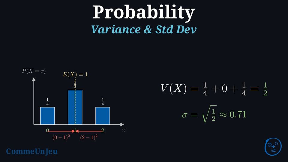
The variance measures how spread out the values of a random variable are from its expected value. The standard deviation is the square root of the variance, giving a sense of typical deviation in the same units as \(X\).
Definition — Variance and Standard Deviation
The variance, denoted \(V(X)\), is:$$\begin{aligned}V(X) &= \sum_{i=1}^{n} (x_i - E(X))^2 P(X = x_i)\\
&= \left(x_1-E(X)\right)^2 P(X = x_1) + \left(x_2-E(X)\right)^2 P(X = x_2) + \cdots + \left(x_n-E(X)\right)^2 P(X = x_n)\\
\end{aligned}$$ The standard deviation, denoted \(\sigma(X)\), is \(\sigma(X) = \sqrt{V(X)}\). Example
You toss 2 fair coins, and \(X\) is the number of heads. The probability table is: | \(x\) | 0 | 1 | 2 |
| \(P(X = x)\) | \(\frac{1}{4}\) | \(\frac{1}{2}\) | \(\frac{1}{4}\) |
Calculate \(V(X)\):$$\begin{aligned}V(X) &= (0 - 1)^2 \times \frac{1}{4} + (1 - 1)^2 \times \frac{1}{2} + (2 - 1)^2 \times \frac{1}{4} \\
&= 1 \times \frac{1}{4} + 0 \times \frac{1}{2} + 1 \times \frac{1}{4} \\
&= \frac{1}{4} + 0 + \frac{1}{4} \\
&= \frac{1}{2} \\
\end{aligned}$$ The variance is \(\frac{1}{2}\).
Proposition — König-Huygens Formula
Let \(X\) take the values \(x_1, \dots, x_n\) with probabilities \(p_1, \dots, p_n\). Writing \(E(X^2) = p_1 x_1^2 + \dots + p_n x_n^2\) for the expected value of the squares, $$V(X) = E(X^2) - [E(X)]^2.$$ The variance is the mean of the squares minus the square of the mean: a formula more convenient than the definition, since it spares the deviations \(x_i - E(X)\).
Write \(\mu = E(X)\). For each value, \((x_i - \mu)^2 = x_i^2 - 2\mu x_i + \mu^2\). Multiplying by \(p_i\) and adding over \(i\): $$\begin{aligned}[t] V(X) &= \sum_{i=1}^{n} p_i (x_i - \mu)^2 && \scriptscriptstyle\text{(definition of the variance)} \\
&= \sum_{i=1}^{n} p_i x_i^2 - 2\mu \sum_{i=1}^{n} p_i x_i + \mu^2 \sum_{i=1}^{n} p_i && \scriptscriptstyle\text{(expanding and splitting the sum)} \\
&= E(X^2) - 2\mu \cdot \mu + \mu^2 \cdot 1 && \scriptscriptstyle\text{(}\sum p_i x_i^2 = E(X^2)\text{, }\sum p_i x_i = \mu\text{, }\sum p_i = 1\text{)} \\
&= E(X^2) - \mu^2 = E(X^2) - [E(X)]^2. \end{aligned}$$
Example
The law of \(X\) is given by the table below. Compute \(V(X)\) with the König-Huygens formula, then check with the definition. | \(x_i\) | \(-2\) | \(0\) | \(3\) | \(10\) |
| \(P(X = x_i)\) | \(0.4\) | \(0.3\) | \(0.2\) | \(0.1\) |
$$\begin{aligned}[t] E(X) &= 0.4 \times (-2) + 0.3 \times 0 + 0.2 \times 3 + 0.1 \times 10 = 0.8 \\
E(X^2) &= 0.4 \times 4 + 0.3 \times 0 + 0.2 \times 9 + 0.1 \times 100 = 13.4 \\
V(X) &= E(X^2) - [E(X)]^2 = 13.4 - 0.64 = 12.76 && \scriptscriptstyle\text{(König-Huygens)} \end{aligned}$$ Check with the definition: \(0.4 \times (-2.8)^2 + 0.3 \times (-0.8)^2 + 0.2 \times 2.2^2 + 0.1 \times 9.2^2 = 3.136 + 0.192 + 0.968 + 8.464 = 12.76\). Hence \(\sigma(X) = \sqrt{12.76} \approx 3.57\).
Proposition — Variance of \(aX + b\)
For any random variable \(X\) and any constants \(a\) and \(b\): $$\textcolor{colorprop}{V(aX + b) = a^2\,V(X)} \qquad \text{and} \qquad \textcolor{colorprop}{\sigma(aX + b) = |a|\,\sigma(X)}.$$ Adding a constant \(b\) moves every value, and the expected value with them, by the same amount: the deviations from the mean do not change, nor does the spread. Multiplying by \(a\) multiplies every deviation by \(a\), hence every squared deviation by \(a^2\). These are the rules already known for the mean and the standard deviation of a linear transformation of data; with the expectation of \(aX + b\), they tell how the centre and the spread of a random variable change when its unit or its origin changes.
Let \(X\) take the values \(x_1, \dots, x_n\) with probabilities \(p_1, \dots, p_n\), and write \(\mu = E(X)\). On the outcomes where \(X\) takes the value \(x_i\), which have probability \(p_i\), the variable \(aX + b\) takes the value \(ax_i + b\); its expected value is \(a\mu + b\) (expectation of \(aX + b\)). The deviation from the mean on these outcomes is therefore \((ax_i + b) - (a\mu + b) = a(x_i - \mu)\). $$\begin{aligned}[t] V(aX + b) &= \sum_{i=1}^{n} p_i \bigl((ax_i + b) - (a\mu + b)\bigr)^2 && \text{(definition of the variance)} \\
&= \sum_{i=1}^{n} p_i\, a^2 (x_i - \mu)^2 && \text{(the deviations are multiplied by } a\text{)} \\
&= a^2 \sum_{i=1}^{n} p_i (x_i - \mu)^2 && \text{(factor out the constant } a^2\text{)} \\
&= a^2\, V(X). \end{aligned}$$ Taking square roots, \(\sigma(aX + b) = \sqrt{a^2\, V(X)} = |a|\,\sigma(X)\), since \(\sqrt{a^2} = |a|\).
Example
- The number \(X\) of items that a market stall sells in a day is a random variable with \(E(X) = 25\) and \(\sigma(X) = 4\). Each item brings \(8\) euros and the stall costs \(60\) euros a day, so the daily gain is \(G = 8X - 60\) euros. Compute \(E(G)\), \(V(G)\) and \(\sigma(G)\).
- A random variable \(X\) has \(E(X) = 3\) and \(V(X) = 4\). Compute \(E(Y)\) and \(\sigma(Y)\) for \(Y = 10 - 2X\).
- \(G = aX + b\) with \(a = 8\) and \(b = -60\). $$\begin{aligned}[t] E(G) &= 8\,E(X) - 60 && \text{(expectation of } aX + b\text{)} \\ &= 8 \times 25 - 60 = 140, \\ V(G) &= 8^2\,V(X) && \text{(variance of } aX + b\text{)} \\ &= 64 \times 4^2 = 1\,024, \\ \sigma(G) &= |8| \times \sigma(X) = 8 \times 4 = 32. \end{aligned}$$ The mean gain is computed like any gain, \(8 \times 25 - 60 = 140\) euros; the spread is only multiplied by \(8\), and the fixed cost \(60\) plays no part in it.
- \(Y = aX + b\) with \(a = -2\) and \(b = 10\). $$\begin{aligned}[t] E(Y) &= -2\,E(X) + 10 = -2 \times 3 + 10 = 4, \\ V(Y) &= (-2)^2\,V(X) = 4 \times 4 = 16, \\ \sigma(Y) &= \sqrt{16} = 4. \end{aligned}$$ Check: \(\sigma(X) = \sqrt{4} = 2\) and \(|-2| \times 2 = 4\). A negative factor reverses the order of the values, not their spread: the standard deviation is multiplied by \(|a| = 2\) and stays positive.
Skills to practice
- Calculating Standard Deviations
- Computing the Mean and Variance of \(aX + b\)
III
Repeated Trials
III.1
Independent Trials and Bernoulli Trials
The Same Urn, Two Draws
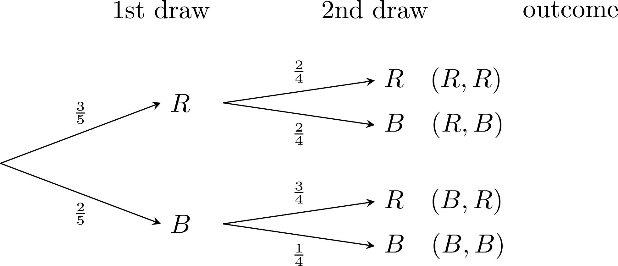
An urn holds three red balls and two blue balls, indistinguishable by touch. A ball is drawn, its colour is noted, then a second ball is drawn. 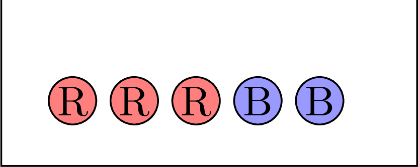
An urn: three red balls, two blue balls
An urn: three red balls, two blue balls
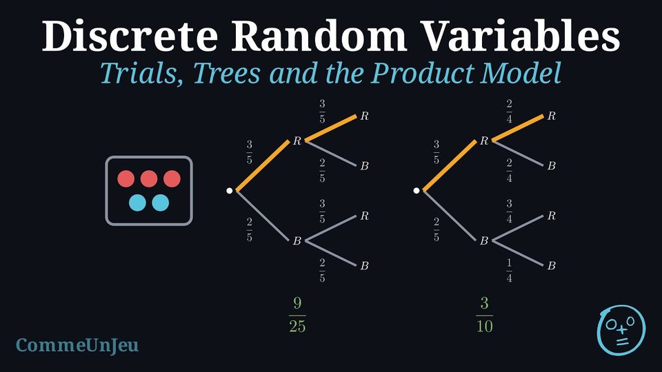
- With replacement, the first ball goes back into the urn: the second draw has the same probabilities as the first, \(\frac{3}{5}\) for red and \(\frac{2}{5}\) for blue, whatever the first result. The two draws do not influence each other: they are independent. The probability of the outcome (red, red) is \(\frac{3}{5} \times \frac{3}{5} = \frac{9}{25}\).
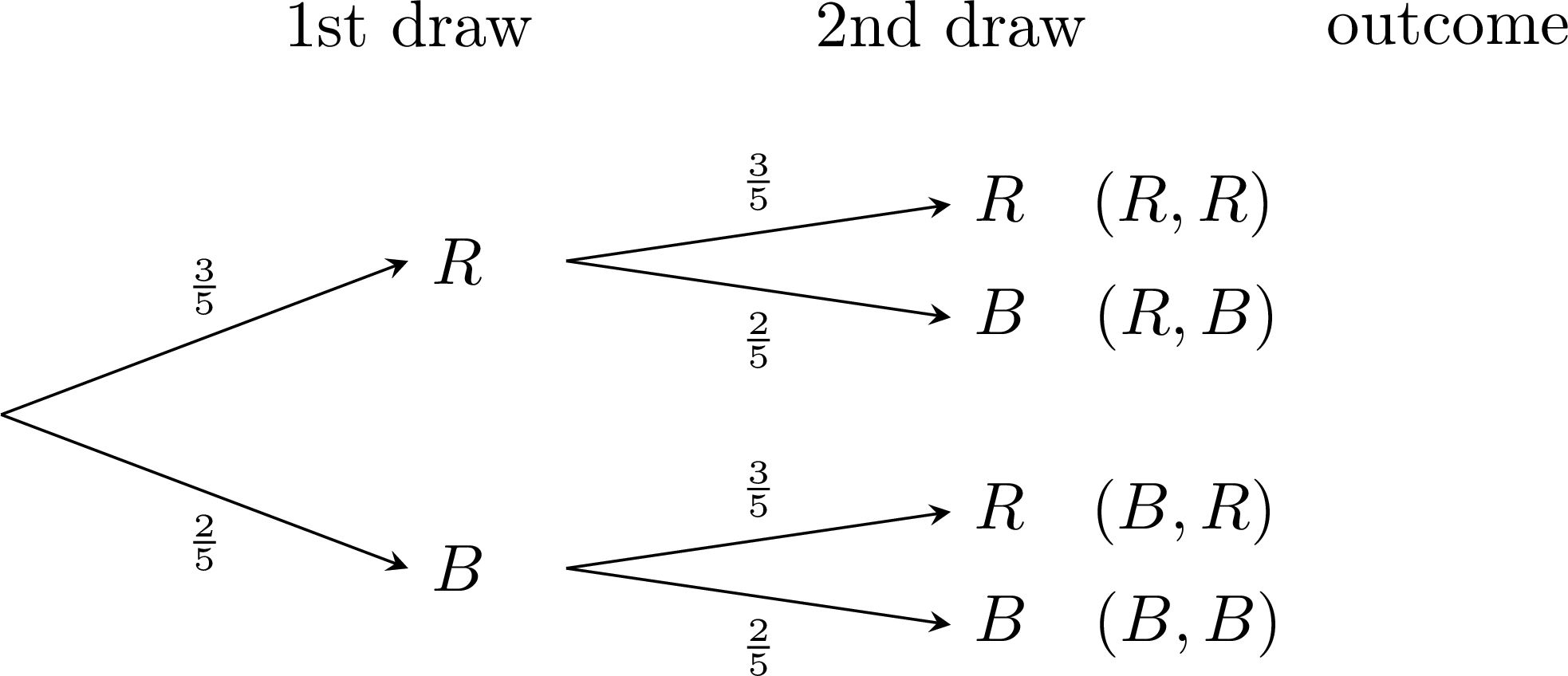
- Without replacement, the first ball stays out: the probabilities of the second draw depend on the first result, \(\frac{2}{4}\) for red after a red ball, \(\frac{3}{4}\) after a blue one. The two draws are not independent; the branches carry conditional probabilities, and the probability of (red, red) is \(\frac{3}{5} \times \frac{2}{4} = \frac{3}{10}\).
Definition — Sequence of Trials
A sequence of \(n\) trials is a random experiment made of \(n\) random experiments performed one after the other, with sets of outcomes \(E_1, E_2, \dots, E_n\). An outcome of the sequence is the list \((x_1, x_2, \dots, x_n)\) of the results, with \(x_i \in E_i\); the sample space is the Cartesian product \(E_1 \times E_2 \times \dots \times E_n\) of all these lists. The sequence is represented by a tree with \(n\) levels, one per trial: a path from the root to a leaf is an outcome. Definition — Independent Trials: the Product Model
The \(n\) trials are independent when the result of any of them does not depend on the results of the others: on the tree, each outcome of a trial keeps the same probability whatever the results of the previous trials, so, at a given level of the tree, the branches leading to the same outcome carry the same weight whatever the node they leave from (the weights of the different outcomes of one trial need not be equal). In this model, the probability of an outcome is the product of the probabilities of its components: $$P\bigl((x_1, x_2, \dots, x_n)\bigr) = P_1(x_1) \times P_2(x_2) \times \dots \times P_n(x_n),$$ where \(P_i(x_i)\) is the probability of the result \(x_i\) in the \(i\)-th trial. For two trials, this is the multiplication rule for independent events.
A Model, Not a Theorem
Independence is an assumption about the situation, chosen when the trials do not influence each other: draws with replacement, repeated tosses of a coin, repeated shots of a player whose form does not change. In a given situation it is a modelling choice, stated rather than deduced from the data: the product formula then defines the probability model of the sequence. The independence is mutual: it concerns all the trials together, not only two by two.
Definition — Bernoulli Trial
A Bernoulli trial is a random experiment with exactly two outcomes, called success (\(S\)) and failure (\(F\)). The probability of success is a number \(p\) strictly between \(0\) and \(1\) — a success that is neither impossible nor certain; the probability of failure is then \(1 - p\). 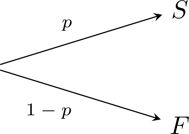
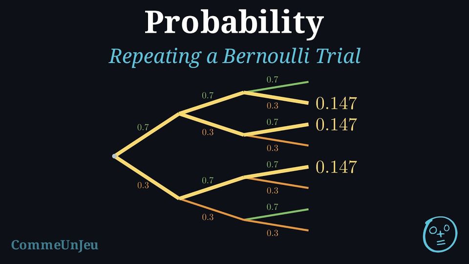
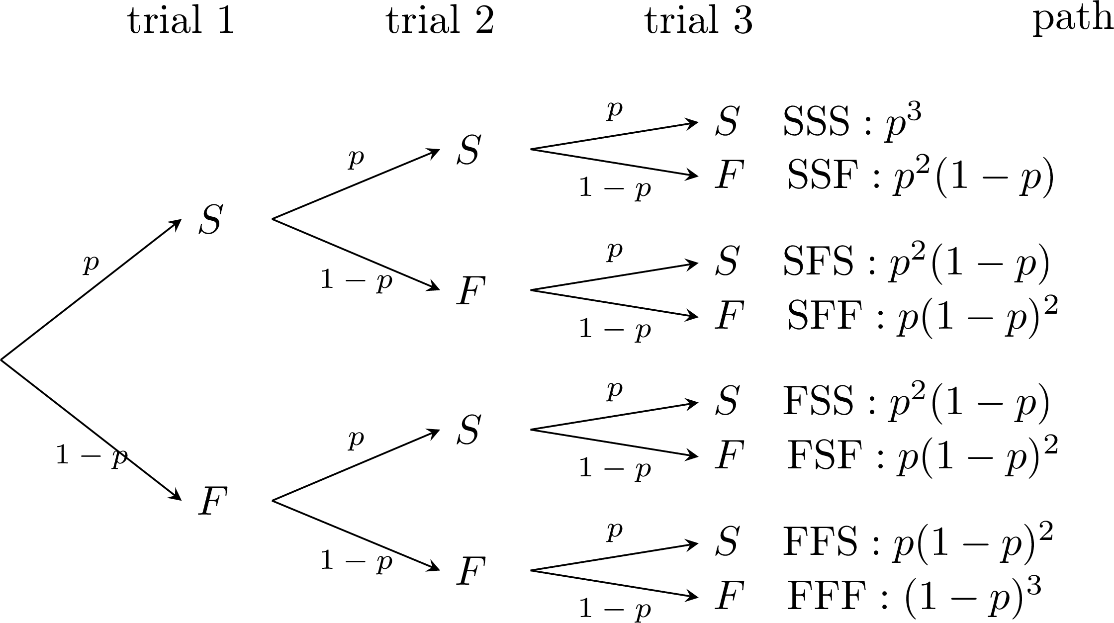
Repeating the trial. The same Bernoulli trial is now repeated \(n\) times, the repetitions being identical (the probability of success is \(p\) at every trial) and independent (whatever the outcomes of the previous trials, the probability of success at the next one is still \(p\)) — this repetition is also called a Bernoulli scheme. An outcome of the whole experiment is a list of \(n\) letters \(S\) or \(F\), one per trial, and the tree of the experiment has \(2^n\) paths: \(4\) for two trials, \(8\) for three, \(16\) for four. By independence, the probability of a path is the product of the probabilities written on its branches: a path with \(k\) successes and \(n - k\) failures, in any order, has probability \(p^k (1 - p)^{n - k}\).
Method — Computing a Probability with the Tree
For \(n \leq 4\) repetitions of a Bernoulli trial: - Draw the tree, one level per trial, with \(p\) on every success branch and \(1 - p\) on every failure branch (the same numbers at every level, since the trials are identical and independent).
- Select the paths that make up the event: for instance “exactly two successes” selects the paths that contain exactly two letters \(S\).
- Multiply along each path, then add the selected paths: all the paths with the same number of successes have the same probability, so it is enough to count them.
Example
A basketball player scores a free throw with probability \(0.7\). She shoots three free throws, independently. - Draw the tree of the experiment.
- Compute the probability that she scores exactly two of the three.
- Compute the probability that she scores at least one.
- Each throw is a Bernoulli trial with success \(S\) (“scored”) of probability \(0.7\) and failure \(F\) of probability \(0.3\); three identical independent trials give a tree with \(8\) paths.
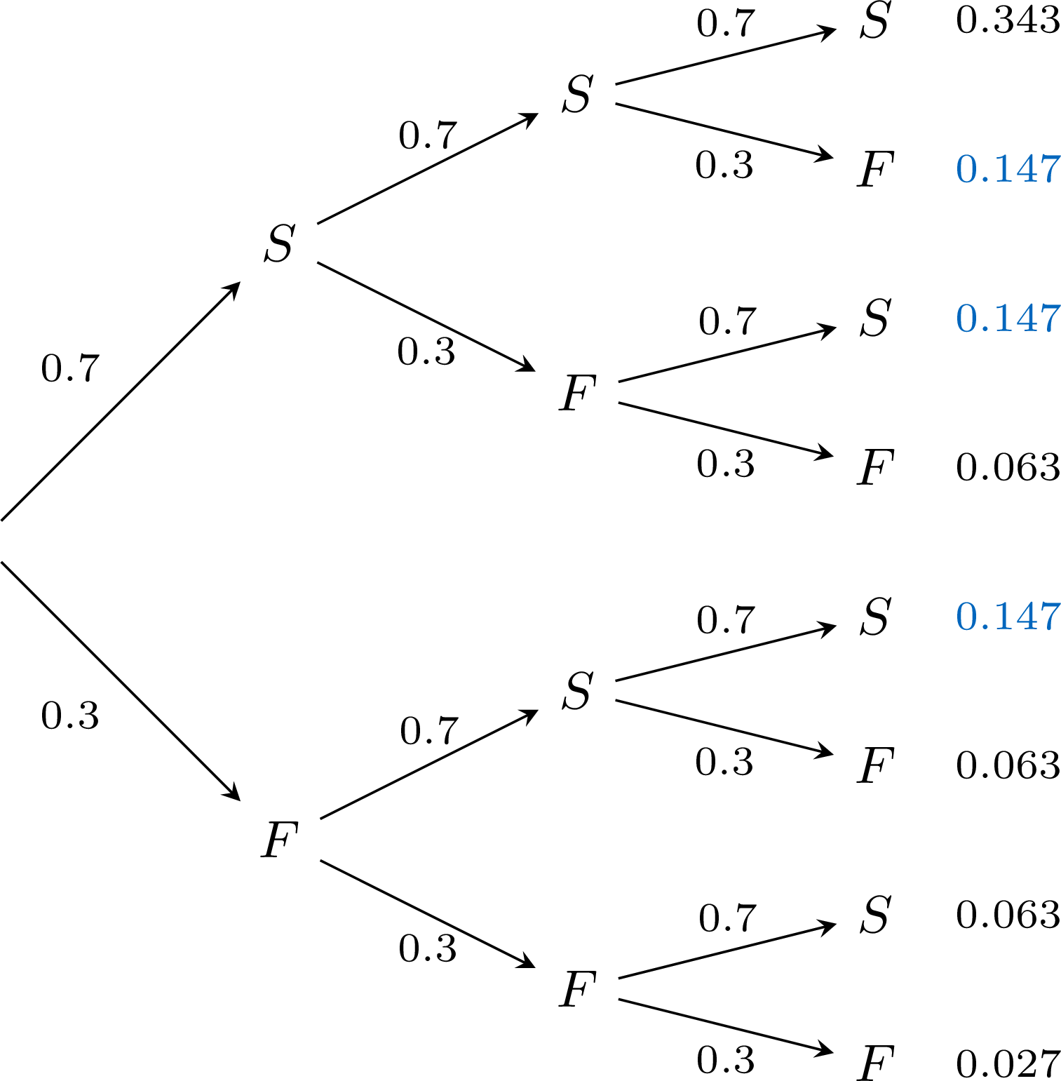
- “Exactly two scored” is made of the three paths \(SSF\), \(SFS\) and \(FSS\), each of probability \(0.7 \times 0.7 \times 0.3 = 0.147\): \(P = 3 \times 0.147 = 0.441\).
- “At least one scored” is the complement of “none scored”, the single path \(FFF\) of probability \(0.3^3 = 0.027\): \(P = 1 - 0.027 = 0.973\).
Example
A fair coin is tossed four times, the tosses being independent. Without drawing the whole tree, compute the probability of getting exactly two heads.
Each toss is a Bernoulli trial with success “heads” of probability \(\dfrac{1}{2}\); the four tosses are identical and independent, and the tree has \(2^4 = 16\) paths, each of probability \(\left(\dfrac{1}{2}\right)^4 = \dfrac{1}{16}\). The paths with exactly two heads are those where the two letters \(S\) occupy two of the four positions: \(SSFF\), \(SFSF\), \(SFFS\), \(FSSF\), \(FSFS\), \(FFSS\) — six paths. Hence \(P = \dfrac{6}{16} = \dfrac{3}{8} = 0.375\). Listing the paths replaces the drawing: with four trials the tree is already wide, and beyond four the count of paths needs a tool of its own.
Skills to practice
- Recognising a Bernoulli Trial
- Computing with the Tree
- Solving Problems with the Tree
IV
The Bernoulli, Binomial and Poisson Distributions
IV.1
The Bernoulli Distribution
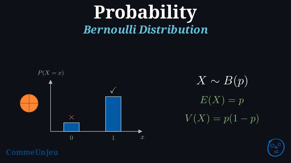
A Bernoulli trial produces a random variable: \(X = 1\) if the trial is a success, \(X = 0\) if it is a failure. Its distribution is the Bernoulli distribution with parameter \(p\), the probability of success.
Definition — Bernoulli Distribution
A random variable \(X\) follows a Bernoulli distribution with parameter \(p\) if: - Possible values are 0 and 1.
- \(P(X = 1) = p\) and \(P(X = 0) = 1 - p\).
Example
A basketball player has an 80\(\pourcent\) chance of making a free throw. Let \(X = 1\) if the shot is made, and \(X = 0\) if it’s missed. - Does \(X\) follow a Bernoulli distribution?
- Find the probability of success.
- Yes, \(X\) has values 0 or 1, so it follows a Bernoulli distribution.
- Probability of success: \(P(X = 1) = 80\pourcent = 0.8\).
Proposition — Expectation and Variance of a Bernoulli Distribution
For a Bernoulli random variable \(X\) with a probability of success \(p\), the following hold: - The expected value is \(E(X) = p\),
- The variance is \(V(X) = p(1 - p)\),
- The standard deviation is \(\sigma(X) = \sqrt{p(1 - p)}\).
- \(\begin{aligned}[t]E(X)&=0\times P(X=0)+1\times P(X=1)\\&=0\times(1-p)+1\times p\\&=p\end{aligned}\)
- \(\begin{aligned}[t] V(X) &= (0-p)^2(1-p) + (1-p)^2 p \\ &= p^2(1-p) + p(1-p)^2 \\ &= p(1-p) [p + (1-p)] \\ &= p(1-p) \\ \end{aligned} \)
Skills to practice
- Identifying Bernoulli Distributions
IV.2
The Binomial Distribution
Definition — Bernoulli Scheme
A Bernoulli scheme with parameters \(n\) and \(p\) is the sequence of \(n\) Bernoulli trials that are identical (same probability of success \(p\)) and independent: the same trial repeated \(n\) times, without any trial influencing the others. It is recognised by four conditions: - a fixed number \(n\) of trials;
- each trial has two outcomes, success and failure;
- the probability of success \(p\) is the same at every trial;
- the trials are independent.
Definition — Binomial Distribution
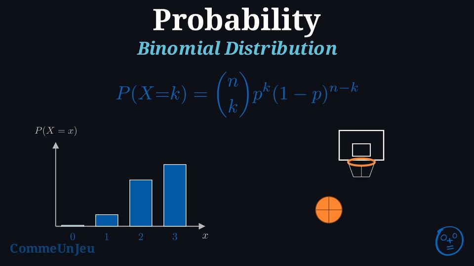
In a Bernoulli scheme with parameters \(n\) and \(p\), let \(X\) be the number of successes. \(X\) takes the values \(0, 1, \dots, n\); its probability distribution is called the binomial distribution with parameters \(n\) and \(p\), written \(\mathcal{B}(n, p)\), and we write \(X \sim \mathcal{B}(n, p)\). Proposition — Probability of \(k\) Successes
Let \(X \sim \mathcal{B}(n, p)\). The probability distribution of \(X\) is: 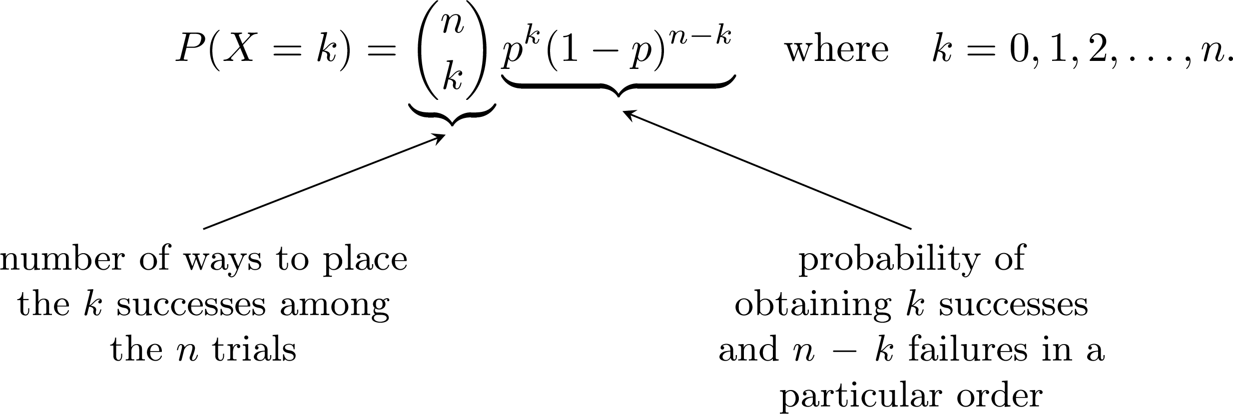
Example
A basketball player has an 80\(\pourcent\) chance of making a free throw and takes 5 shots; the shots are assumed to be independent of one another. Let \(X\) be the number of shots made. - Does \(X\) follow a binomial distribution?
- Find the probability of making 4 shots.
- Yes, \(X\) follows a binomial distribution because it counts the number of successes (shots made) in 5 independent trials (free throws), each with a constant success probability of 0.8.
- As \(X \sim \mathcal{B}(5, 0.8)\), $$ \begin{aligned} P(X = 4) &= \binom{5}{4} (0.8)^4 (1-0.8)^1 \\ &= 5 \times 0.4096 \times 0.2 \\ &= 0.4096 \end{aligned} $$ The probability of making 4 out of 5 shots is \(0.4096 = 40.96\pourcent\).
Proposition — Expectation and Variance of a Binomial Distribution
For \(X \sim \mathcal{B}(n, p)\): - \(E(X) = n p\) (expected value),
- \(V(X) = n p (1 - p)\) (variance),
- \(\sigma(X) = \sqrt{n p (1 - p)}\) (standard deviation).
Example
- A machine makes defective parts with probability \(0.02\), independently from one part to the next. In a batch of \(150\) parts, \(X\) counts the defective ones. Give the distribution of \(X\), then \(E(X)\), and interpret it.
- A seed germinates with probability \(0.85\). Forty seeds are sown, independently. How many germinated seeds can be expected on average?
- Each part is a Bernoulli trial (success: “defective”, \(p = 0.02\)), repeated \(150\) times independently: \(X \sim \mathcal{B}(150, 0.02)\). Then \(E(X) = 150 \times 0.02 = 3\): over many batches, a batch contains on average \(3\) defective parts.
- \(X \sim \mathcal{B}(40, 0.85)\) and \(E(X) = 40 \times 0.85 = 34\): about \(34\) germinated seeds on average.
The Bar Chart of a Binomial Distribution
The bar chart of \(X \sim \mathcal{B}(n, p)\) shows the probabilities \(P(X = k)\) for \(k = 0, 1, \dots, n\). Its highest bar stands close to the expected value \(E(X) = np\). When \(np\) and \(n(1-p)\) are not too small, the chart is roughly bell-shaped and centred on \(np\): the bars rise, peak near \(np\), then fall roughly symmetrically. When \(np\) (or \(n(1-p)\)) is small, which happens for a given \(n\) when \(p\) is close to \(0\) (or to \(1\)), the chart loses its symmetry: it is pushed against the edge, its tallest bars stand at the very start (or the very end) and it falls quickly on one side only. Below, \(\mathcal{B}(20, 0.6)\) with \(E(X) = 12\), and \(\mathcal{B}(20, 0.05)\) with \(E(X) = 1\). 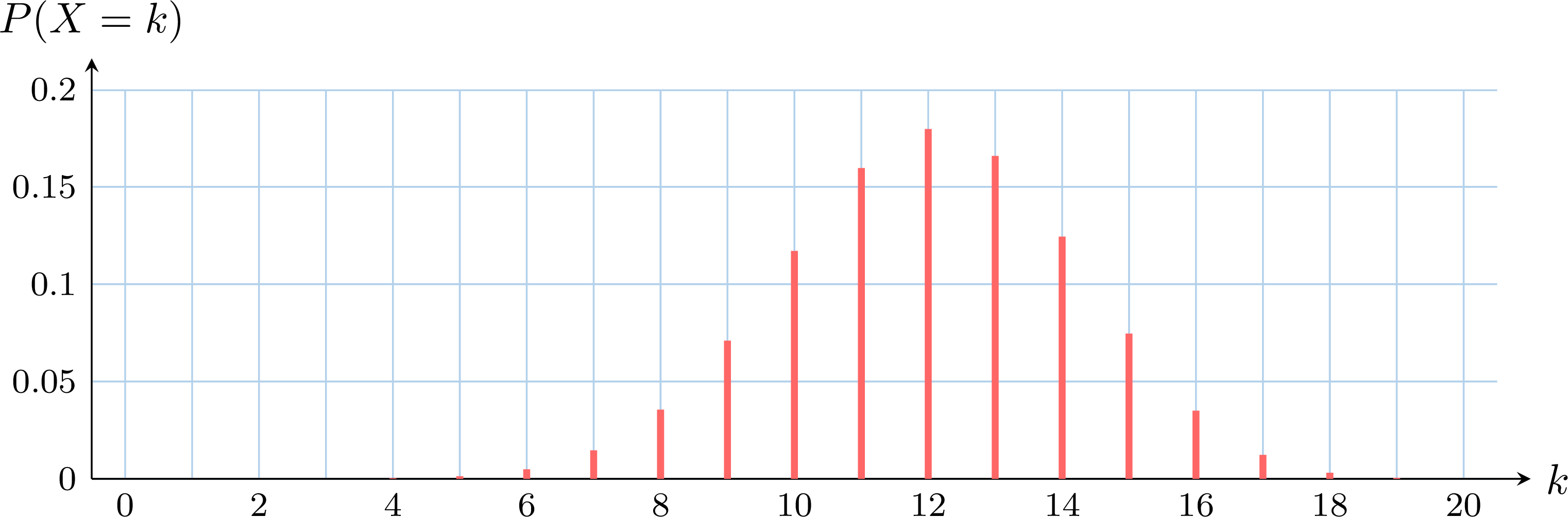
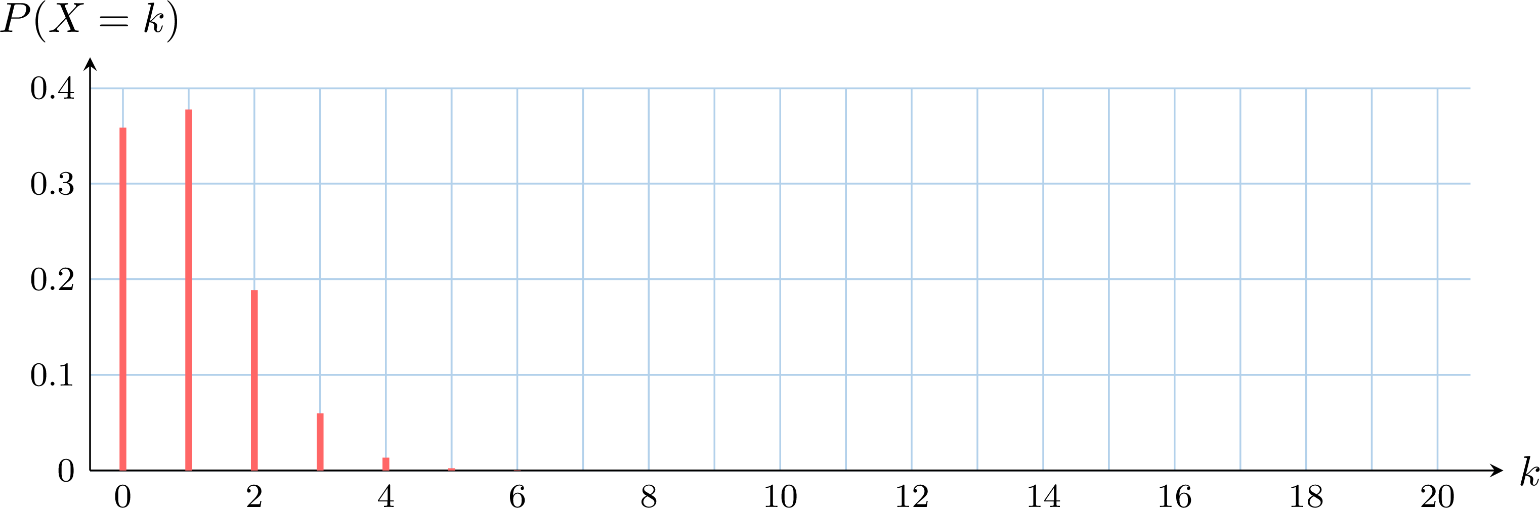
Reading a bar chart the other way round gives information about the parameters: the abscissa of the highest bar is close to \(np\), so it gives an estimate of \(n\) when \(p\) is known, or of \(p\) when \(n\) is known.
Skills to practice
- Identifying Binomial Distributions
- Computing Binomial Probabilities and Expected Values
- Computing the Variance of a Binomial Distribution
IV.3
Binomial Probabilities with Technology
Method — Cumulative Binomial Distribution
To calculate binomial probabilities, we use a graphing calculator: its probability function (PDF) gives \(P(X = k)\), and its Cumulative Distribution Function (CDF) gives probabilities of the form \(P(X \leq k)\). - On TI: Use
binompdf(n, p, k)for \(P(X = k)\) andbinomcdf(n, p, k)for \(P(X \leq k)\). - On Casio: Use
BinomialPD(k, n, p)andBinomialCD(k, n, p). - On NumWorks: Use the
Probabilityapplication, selectBinomial.
- \(P(X < k) = P(X \leq k-1)\)
- \(P(X \geq k) = 1 - P(X \leq k-1)\)
- \(P(X > k) = 1 - P(X \leq k)\)
- \(P(a \leq X \leq b) = P(X \leq b) - P(X \leq a-1)\)
Example
Consider a random variable \(X\) that follows the binomial distribution with parameters \(n = 100\) and \(p = 0.78\). Calculate the following probabilities. Round your results to three decimal places. $$P(X < 75), P(X > 79), P(X \geq 74), P(73 < X \leq 81)$$
With \(X \sim \mathcal{B}(100, 0.78)\), we use the calculator's cumulative distribution function:
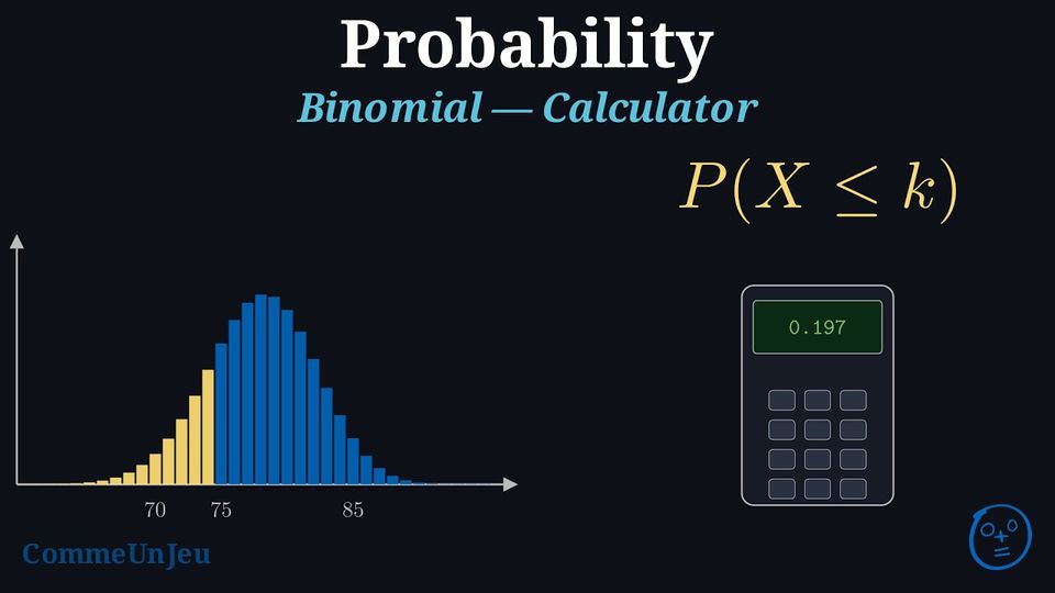
- \(P(X<75) = P(X\leq 74) \approx \mathbf{0.197}\).
- \(P(X>79) = 1 - P(X\leq 79) \approx \mathbf{0.366}\).
- \(P(X\geq 74) = 1 - P(X\leq 73) \approx \mathbf{0.861}\).
- \(P(73
Method — Finding a Threshold
To find the smallest integer \(k\) such that \(P(X \leq k) \geq 1-\alpha\) (where \(\alpha\) is a small value like \(0.05\)), we use the Inverse Binomial function or a table of values on the calculator. Example
Let \(X \sim \mathcal{B}(50, 0.4)\). Find the smallest integer \(k\) such that \(P(X \leq k) \geq 0.95\).
Using the calculator's table of values:
- \(P(X \leq 24) \approx 0.9022\)
- \(P(X \leq 25) \approx 0.9427\)
- \(P(X \leq 26) \approx 0.9686\)
Skills to practice
- Computing Cumulative Binomial Probabilities with Technology
- Finding a Threshold
IV.4
The Poisson Distribution
Counting Events in an Interval
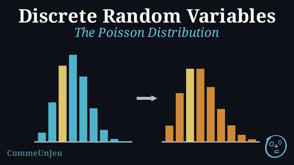
Many random variables count events that occur at random within an interval of time or of space: the calls that reach a help desk in an hour, the typing errors on a page, the flaws along a metre of cable, the patients who arrive at an emergency department during a night. Such a count has no fixed number of trials and no maximum written in advance; what is known is its average rate, the mean number \(\lambda\) of events per interval. A binomial model can still approach it. Suppose the calls arrive independently of one another, at a constant average rate of \(\lambda = 3\) per hour, and cut the hour into \(n\) equal slots, so short that two calls hardly ever fall in the same slot. Each slot then behaves almost like a Bernoulli trial, of success “a call in this slot” and probability \(\dfrac{3}{n}\), the slots being independent, and the number of calls is close to \(\mathcal{B}\left(n, \dfrac{3}{n}\right)\) — the closer as the slots get shorter. For these binomial distributions, the probability of exactly \(2\) calls settles:
The limit of these binomial distributions is a distribution of its own, which depends only on the rate \(\lambda\): the Poisson distribution.
| \(n\) | \(10\) | \(100\) | \(1000\) | limit |
| \(P(X = 2)\) | \(0.2335\) | \(0.2252\) | \(0.2242\) | \(0.2240\) |
Definition — Poisson Distribution
Let \(\lambda\) be a positive real number. A random variable \(X\) follows the Poisson distribution with parameter \(\lambda\) if it takes the values \(0, 1, 2, 3, \dots\) (every natural number) and, for each of them, $$P(X = k) = \frac{e^{-\lambda}\,\lambda^k}{k!},$$ where \(k! = 1 \times 2 \times \dots \times k\) (read “\(k\) factorial”) for \(k \geq 1\), and \(0! = 1\). We write \(X \sim \mathcal{P}(\lambda)\); many textbooks write \(X \sim \mathrm{Po}(\lambda)\). The parameter \(\lambda\) is the mean number of events in the interval. \(X\) is a discrete random variable with infinitely many values, and these probabilities add up to \(1\) (admitted). Method — Recognising a Poisson Model
A random variable \(X\) is modelled by a Poisson distribution when: - \(X\) counts events in a fixed interval of time or of space (an hour, a page, a metre, a square kilometre) — not successes among a fixed number of trials;
- the events occur independently of one another: an event does not make another one more or less likely;
- the events occur at a uniform average rate over the interval: the mean number of events is proportional to the size of the interval (its length, its area or its volume).
Proposition — Expectation and Variance of a Poisson Distribution
If \(X \sim \mathcal{P}(\lambda)\), then $$\textcolor{colorprop}{E(X) = \lambda}, \qquad \textcolor{colorprop}{V(X) = \lambda} \qquad \text{and} \qquad \sigma(X) = \sqrt{\lambda}.$$ The mean and the variance of a Poisson distribution are equal. These results are admitted; the binomial distributions \(\mathcal{B}\left(n, \dfrac{\lambda}{n}\right)\) whose limit is \(\mathcal{P}(\lambda)\) make them plausible, with mean \(n \times \dfrac{\lambda}{n} = \lambda\) and variance \(n \times \dfrac{\lambda}{n}\left(1 - \dfrac{\lambda}{n}\right) = \lambda\left(1 - \dfrac{\lambda}{n}\right)\), which gets closer to \(\lambda\) as \(n\) grows. The equality gives a first check on data: counts whose mean and variance are clearly different are not well modelled by a Poisson distribution. Example
The typing errors in a report occur independently, at a constant average rate of \(1.8\) per page. Let \(X\) be the number of errors on a page chosen at random. - Give the distribution of \(X\), its expected value and its standard deviation.
- Compute \(P(X = 0)\) and \(P(X = 2)\).
- Compute the probability that the page contains at least two errors.
- \(X\) counts events in a fixed interval (a page), which occur independently at a uniform average rate: \(X \sim \mathcal{P}(1.8)\). Hence \(E(X) = 1.8\) errors and \(\sigma(X) = \sqrt{1.8} \approx 1.34\).
- By the formula \(P(X = k) = \dfrac{e^{-\lambda}\lambda^k}{k!}\) with \(\lambda = 1.8\): $$\begin{aligned}[t] P(X = 0) &= \frac{e^{-1.8} \times 1.8^0}{0!} = e^{-1.8} \approx 0.165, \\ P(X = 2) &= \frac{e^{-1.8} \times 1.8^2}{2!} = 1.62\,e^{-1.8} \approx 0.268. \end{aligned}$$
- “At least two” is the complement of “zero or one”, and \(P(X = 1) = 1.8\,e^{-1.8}\): $$\begin{aligned}[t] P(X \geq 2) &= 1 - P(X = 0) - P(X = 1) && \text{(complement)} \\ &= 1 - e^{-1.8} - 1.8\,e^{-1.8} \\ &= 1 - 2.8\,e^{-1.8} \approx 0.537. \end{aligned}$$
Method — Poisson Probabilities with Technology
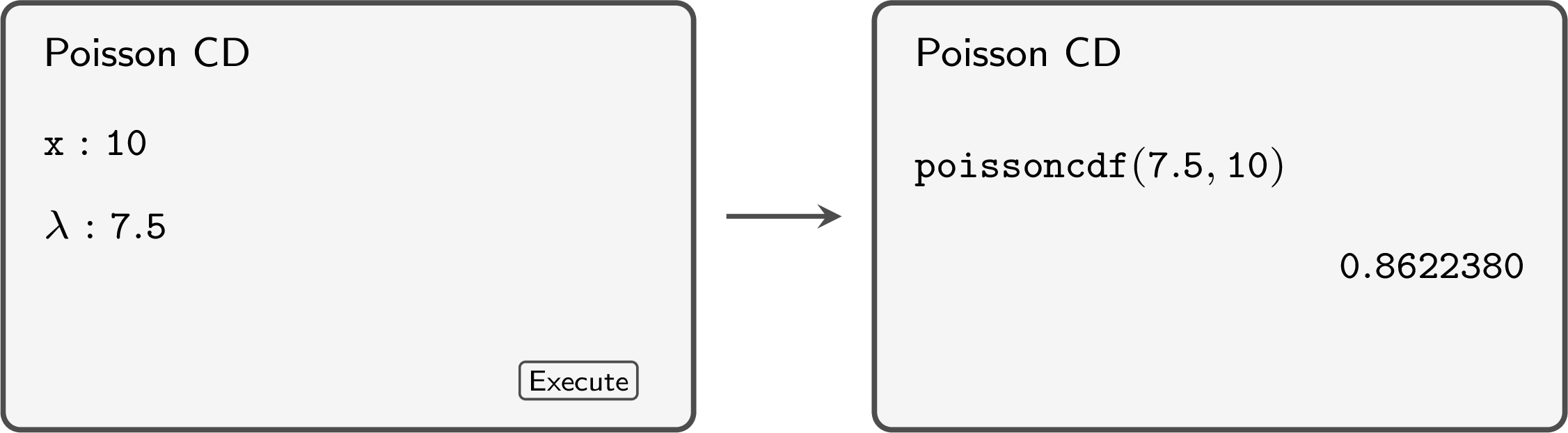
For \(X \sim \mathcal{P}(\lambda)\), a graphing calculator gives the two kinds of probabilities directly. Their names depend on the calculator: Poisson P.D and Poisson C.D, poissonpdf and poissoncdf. - State the model \(X \sim \mathcal{P}(\lambda)\), with \(\lambda\) the mean number of events in the interval of the question.
- One value: the probability function (P.D,
poissonpdf) gives \(P(X = k)\). - Cumulative probability: the cumulative function (C.D,
poissoncdf) gives \(P(X \leq k)\). The other events are written with it, \(k\), \(a\) and \(b\) being whole numbers with \(a \leq b\): $$\begin{aligned} P(X < k) &= P(X \leq k - 1), & P(X \geq k) &= 1 - P(X \leq k - 1), \\ P(X > k) &= 1 - P(X \leq k), & P(a \leq X \leq b) &= P(X \leq b) - P(X \leq a - 1). \end{aligned}$$ - Threshold: the smallest whole number \(k\) such that \(P(X \leq k) \geq 0.95\) (or any other level) is read in a table of values of the cumulative function, \(k = 0, 1, 2, \dots\)
Example
A taxi company receives bookings independently, at a constant average rate of \(10\) per hour. - Compute the probability of at most \(2\) bookings in \(12\) minutes.
- Compute the probability of more than \(15\) bookings in an hour.
- How many bookings must the company be able to serve in an hour so that the demand of that hour is met with probability at least \(0.95\)?
- The rate is uniform, so over \(12\) minutes the mean is \(\lambda = 10 \times \dfrac{12}{60} = 2\): the number \(Q\) of bookings follows \(\mathcal{P}(2)\), and the cumulative function gives \(P(Q \leq 2) \approx 0.677\).
- Over an hour, the number \(H\) of bookings follows \(\mathcal{P}(10)\): $$\begin{aligned}[t] P(H > 15) &= 1 - P(H \leq 15) && \text{(complement)} \\ &\approx 1 - 0.9513 \approx 0.0487. \end{aligned}$$
- We need the smallest whole number \(k\) such that \(P(H \leq k) \geq 0.95\). The table of values of the cumulative function gives \(P(H \leq 14) \approx 0.917 < 0.95\) and \(P(H \leq 15) \approx 0.951 \geq 0.95\): the company must be able to serve \(15\) bookings in the hour.
Method — Choosing Between the Binomial and Poisson Models
Both distributions count, but not the same thing. - Binomial \(\mathcal{B}(n, p)\): \(X\) counts the successes among a fixed number \(n\) of identical independent trials; its values stop at \(n\); its parameters are \(n\) and the probability of success \(p\).
- Poisson \(\mathcal{P}(\lambda)\): \(X\) counts events in an interval, with no fixed number of trials and no maximum; its only parameter is the mean number \(\lambda\) of events in the interval.
Skills to practice
- Recognising a Poisson Model
- Computing Poisson Probabilities
- Modelling with a Poisson Distribution
V
Going further
Skills to practice
- Solving Problems
- Problems: Working with Poisson Counts
- Quiz
Jump to section