International Baccalaureate · DP 2: Applications and Interpretation HL

Estimation and Confidence Intervals

⌚ ~178 min ▢ 20 blocks ✓ 88 exercises ➣ Prerequisites : Discrete Random Variables, The Normal Distribution

I Linear Combinations of Random Variables

I.1 Expectation and Variance of a Combination

Consider flipping a fair coin two times. Let the random variables $X_1$ and $X_2$ represent the outcome of the first and second coin flips, respectively. We code success (Heads) as 1 and failure (Tails) as 0. We assume the two flips are independent.
Thus, $X_1$ and $X_2$ follow a Bernoulli distribution with probability of success $p=\dfrac{1}{2}$. We are interested in two new random variables:

$S_2 = X_1 + X_2$: the total number of heads.
$\overline{X}_2 = \dfrac{X_1 + X_2}{2}$: the average proportion of heads.

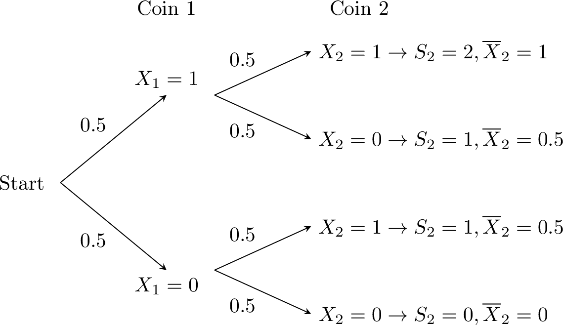
Probability distribution: We can visualize the outcomes using a probability tree. The probability distributions are:

$s$ (Sum) $0$ $1$ $2$

$P(S_2=s)$ $1/4$ $1/2$ $1/4$

$\bar{x}$ (Mean) $0$ $0.5$ $1$

$P(\overline{X}_2=\bar{x})$ $1/4$ $1/2$ $1/4$
Expectation:$$E(S_2) = 0\left(\tfrac{1}{4}\right) + 1\left(\tfrac{1}{2}\right) + 2\left(\tfrac{1}{4}\right) = 1,$$ $$E(\overline{X}_2) = 0\left(\tfrac{1}{4}\right) + 0.5\left(\tfrac{1}{2}\right) + 1\left(\tfrac{1}{4}\right) = 0.5.$$
Connection to individual variables:
Since $E(X_1) = E(X_2) = p = 0.5$, we have:$$E(S_2) = 1 = 2 \times 0.5 = 2E(X_1),$$ $$E(\overline{X}_2) = 0.5 = E(X_1).$$
Variance:$$V(S_2) = (0-1)^2\left(\tfrac{1}{4}\right) + (1-1)^2\left(\tfrac{1}{2}\right) + (2-1)^2\left(\tfrac{1}{4}\right) = \tfrac{1}{4} + 0 + \tfrac{1}{4} = 0.5,$$ $$V(\overline{X}_2) = (0-0.5)^2\left(\tfrac{1}{4}\right) + (0.5-0.5)^2\left(\tfrac{1}{2}\right) + (1-0.5)^2\left(\tfrac{1}{4}\right) = \tfrac{0.25}{4} + 0 + \tfrac{0.25}{4} = 0.125.$$
Connection to individual variance:
Since $V(X_1) = p(1-p) = 0.25$, it follows that:$$V(S_2) = 0.5 = 2 \times 0.25 = 2V(X_1),$$ $$V(\overline{X}_2) = 0.125 = \frac{0.25}{2} = \frac{V(X_1)}{2}.$$

This example suggests general rules for sums and means of independent random variables.

Definition — Linear Combination of Random Variables

A linear combination of random variables $X_1, X_2, \ldots, X_n$ is a new random variable $Y$ defined as$$ Y = a_1 X_1 + a_2 X_2 + \ldots + a_n X_n, $$ where $a_1, a_2, \ldots, a_n$ are constant coefficients.

Definition — Sum and Mean of Random Variables

Given $n$ random variables $X_1, X_2, \dots, X_n$:

The sum is denoted $S_n = X_1 + X_2 + \ldots + X_n$.
The sample mean is denoted $\overline{X}_n = \dfrac{X_1 + X_2 + \ldots + X_n}{n}$.

Proposition — Properties of Expectation and Variance

For random variables $X_1, \dots, X_n$ and constants $a_1, \dots, a_n$:

Expectation is linear: $$ E\left(\sum_{i=1}^n a_i X_i\right) = \sum_{i=1}^n a_i E(X_i). $$
Variance adds for independent variables: if $X_1, \dots, X_n$ are independent, $$ V\left(\sum_{i=1}^n a_i X_i\right) = \sum_{i=1}^n a_i^2 V(X_i). $$

Proposition — Expectation of Sums and Means

If $X_1, X_2, \dots, X_n$ are identically distributed with mean $\mu$, then:$$ E(S_n) = n\mu \qquad\text{and}\qquad E(\overline{X}_n) = \mu. $$

Proof

For the sum $S_n$:
Using linearity of expectation,$$ \begin{aligned}E(S_n) &= E(X_1 + X_2 + \dots + X_n) \\ &= E(X_1) + E(X_2) + \dots + E(X_n) \\ &= \mu + \mu + \dots + \mu \quad \text{($n$ times)} \\ &= n\mu.\end{aligned} $$
For the mean $\overline{X}_n$:
Using $E(aX) = aE(X)$,$$ \begin{aligned}E(\overline{X}_n) &= E\left(\frac{S_n}{n}\right) \\ &= \frac{1}{n} E(S_n) \\ &= \frac{1}{n} (n\mu) \\ &= \mu.\end{aligned} $$

Example

Let $X_1, \dots, X_9$ be random variables with mean $\mu=5$. Find the expected value of their sum $S_9$.

Answer

$$ E(S_9) = 9 \times \mu = 9 \times 5 = 45. $$

Proposition — Variance of Sums and Means

If $X_1, X_2, \dots, X_n$ are independent and identically distributed with variance $\sigma^2$ (and standard deviation $\sigma$), then:

For the sum: $$ V(S_n) = n\sigma^2 \quad \text{and} \quad \sigma(S_n) = \sigma\sqrt{n}; $$
For the mean: $$ V(\overline{X}_n) = \frac{\sigma^2}{n} \quad \text{and} \quad \sigma(\overline{X}_n) = \frac{\sigma}{\sqrt{n}}. $$

Proof

For the sum $S_n$:
Since the variables $X_1, \dots, X_n$ are independent, the variance of the sum is the sum of the variances:$$ \begin{aligned}V(S_n) &= V(X_1 + X_2 + \dots + X_n) \\ &= V(X_1) + V(X_2) + \dots + V(X_n) \\ &= \sigma^2 + \sigma^2 + \dots + \sigma^2 \quad \text{($n$ times)} \\ &= n\sigma^2.\end{aligned} $$ The standard deviation is the square root of the variance:$$ \sigma(S_n) = \sqrt{V(S_n)} = \sqrt{n\sigma^2} = \sigma\sqrt{n}. $$
For the mean $\overline{X}_n$:
Using the property $V(aX) = a^2V(X)$ with $a = \dfrac{1}{n}$,$$ \begin{aligned}V(\overline{X}_n) &= V\left(\frac{S_n}{n}\right) \\ &= \left(\frac{1}{n}\right)^2 V(S_n) \\ &= \frac{1}{n^2} (n\sigma^2) \\ &= \frac{\sigma^2}{n}.\end{aligned} $$ Thus,$$ \sigma(\overline{X}_n) = \sqrt{V(\overline{X}_n)} = \sqrt{\frac{\sigma^2}{n}} = \frac{\sigma}{\sqrt{n}}. $$

Example — Sample Proportion

Items coming off an assembly line are defective with probability $p$. Let $X_i$ be independent indicator variables where $X_i=1$ if the $i$-th item is defective and $0$ otherwise. Then $X_i$ follows a Bernoulli distribution. Find the mean and standard deviation of the sample proportion $\overline{X}_n$.

Answer

For a Bernoulli variable, $\mu = p$ and $\sigma = \sqrt{p(1-p)}$. Therefore, for the sample mean $\overline{X}_n$:$$ E(\overline{X}_n) = p, $$ $$ \sigma(\overline{X}_n) = \frac{\sigma}{\sqrt{n}} = \sqrt{\frac{p(1-p)}{n}}. $$

Example — Combining Two Independent Variables

The random variables $X$ and $Y$ are independent, with $E(X) = 12$, $V(X) = 4$, $E(Y) = 5$ and $V(Y) = 9$.

Find the expected value, the variance and the standard deviation of $2X - 3Y$.
Find $E(X - Y)$ and $V(X - Y)$.
$X_1$ and $X_2$ are two independent variables with the same distribution as $X$. Compare $2X$ and $X_1 + X_2$: their expected values and their variances.

Answer

By the Proposition “Properties of Expectation and Variance”, with the coefficients $2$ and $-3$: $$\begin{aligned}[t] E(2X - 3Y) &= 2E(X) - 3E(Y) && \text{(expectation is linear)} \\ &= 2 \times 12 - 3 \times 5 = 9, \\ V(2X - 3Y) &= 2^2 V(X) + (-3)^2 V(Y) && \text{(independent variables)} \\ &= 4 \times 4 + 9 \times 9 = 97, \end{aligned}$$ so $\sigma(2X - 3Y) = \sqrt{97} \approx 9.85$.
With the coefficients $1$ and $-1$: $$\begin{aligned}[t] E(X - Y) &= E(X) - E(Y) = 12 - 5 = 7, \\ V(X - Y) &= 1^2 V(X) + (-1)^2 V(Y) = 4 + 9 = 13. \end{aligned}$$ The variances add, even for a difference: the coefficient $-1$ is squared, and the variability of $Y$ adds to that of $X$ whatever the sign in front of $Y$.
The expected values are equal: $E(2X) = 2 \times 12 = 24$ and $E(X_1 + X_2) = 12 + 12 = 24$. The variances are not: $$\begin{aligned}[t] V(2X) &= 2^2 V(X) = 16, \\ V(X_1 + X_2) &= V(X_1) + V(X_2) = 4 + 4 = 8 && \text{(independent variables)}. \end{aligned}$$ $2X$ doubles one single value, so its gap to the mean is doubled; in $X_1 + X_2$, the gaps of two independent values partly offset each other. The two variables have the same mean but not the same spread: $2X$ is not $X_1 + X_2$.

Skills to practice

Calculating Expectations and Variances of Combinations
Interpreting Linear Combinations of Random Variables
Calculating Expectation and Variance

I.2 Sum of Independent Poisson Variables

Proposition — Sum of Two Independent Poisson Variables

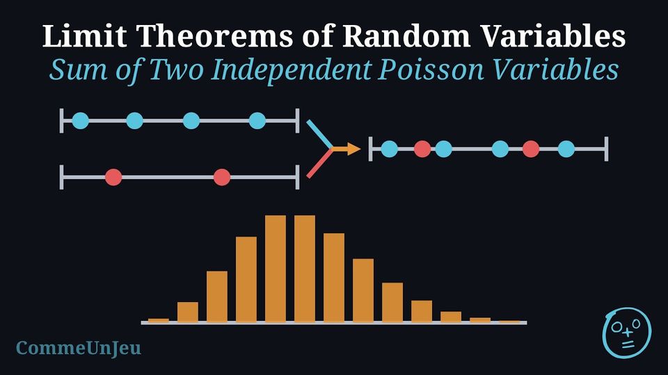
If $X \sim \mathcal{P}(\lambda_1)$ and $Y \sim \mathcal{P}(\lambda_2)$ are independent, then $$X + Y \sim \mathcal{P}(\lambda_1 + \lambda_2).$$ The mean and the variance follow from the Proposition “Properties of Expectation and Variance”: $E(X + Y) = \lambda_1 + \lambda_2$ and, since the variables are independent, $V(X + Y) = \lambda_1 + \lambda_2$ — equal, as for every Poisson variable. That $X + Y$ follows a Poisson distribution is admitted. The result extends to any number of independent Poisson variables: $$X_1 + X_2 + \dots + X_n \sim \mathcal{P}(\lambda_1 + \lambda_2 + \dots + \lambda_n).$$ Both hypotheses matter: the counts are independent, and they are added. The double of a Poisson variable is not a Poisson variable: $E(2X) = 2\lambda_1$ while $V(2X) = 4\lambda_1$, and $2X$ takes only even values.

Example

A help desk receives calls on two lines. The calls on line A arrive independently, at a constant average rate of $3.2$ per hour; the calls on line B arrive independently of line A, at a constant average rate of $1.8$ per hour. The number of calls on each line in a given time is modelled by a Poisson distribution.

Give the distribution of the total number $T$ of calls received in one hour.
Compute $P(T = 4)$ and $P(T \geq 8)$.
Compute the probability that no call is received during a period of $30$ minutes.

Round the probabilities to three significant figures.

Answer

Each line counts events in an interval of one hour, occurring independently at a uniform average rate (Method “Recognising a Poisson Model”): the numbers of calls are $A \sim \mathcal{P}(3.2)$ and $B \sim \mathcal{P}(1.8)$, independent. By the Proposition “Sum of Two Independent Poisson Variables”, $$T = A + B \sim \mathcal{P}(3.2 + 1.8) = \mathcal{P}(5).$$
With $\lambda = 5$: $$\begin{aligned}[t] P(T = 4) &= \frac{e^{-5} \times 5^4}{4!} = \frac{625}{24}\,e^{-5} \approx 0.175, \\ P(T \geq 8) &= 1 - P(T \leq 7) && \text{(complement)} \\ &\approx 1 - 0.8666 \approx 0.133, \end{aligned}$$ $P(T \leq 7)$ being given by the cumulative function (Method “Poisson Probabilities with Technology”).
The rates are uniform, so over $30$ minutes the means are halved: $3.2 \times 0.5 = 1.6$ and $1.8 \times 0.5 = 0.9$. The total number $H$ of calls in $30$ minutes follows $\mathcal{P}(1.6 + 0.9) = \mathcal{P}(2.5)$, and $$P(H = 0) = e^{-2.5} \approx 0.0821.$$

Skills to practice

Using the Sum of Poisson Variables

II Samples and Unbiased Estimates

II.1 Unbiased Estimators of the Mean and the Variance

In most real-world statistical problems, we are interested in understanding the properties of a large population. However, it is often impossible or impractical to collect data from every single member of that population. As a result, we typically do not know the true population parameters, such as the population mean ($\mu$) or the population standard deviation ($\sigma$).
Instead, we collect data from a smaller subset of the population, called a sample. We calculate statistics from this sample (like the sample mean $\bar{x}$) and use them to estimate the unknown population parameters. This process is known as statistical inference. Sampling and estimation rest on a few key concepts.

Report an error

Definition — Sample

A sample of size $n$ consists of $n$ independent random variables $X_1, X_2, \dots, X_n$ that follow the same probability distribution as the population.

Definition — Observed Value

An observed value, denoted by a lowercase $x$, is a specific realization of a random variable $X$. It is the actual number obtained after performing an experiment or collecting data.

Definition — Sample Mean Estimator

The sample mean is a statistic used to estimate the population mean.
Let $X_1, X_2, \dots, X_n$ be a random sample. The sample mean is a random variable denoted by $\overline{X}_n$:$$ \overline{X}_n = \frac{\sum_{i=1}^n X_i}{n} = \frac{X_1 + X_2 + \dots + X_n}{n} $$ For a specific set of observed values $x_1, x_2, \dots, x_n$, the calculated sample mean is denoted by $\bar{x}$:$$ \bar{x} = \frac{\sum_{i=1}^n x_i}{n} $$

Proposition — Unbiased Estimator of the Mean

The sample mean is an unbiased estimator of the population mean $\mu$. This means that the expected value of the sample mean is equal to the true population mean:$$ E[\overline{X}_n] = \mu $$

Definition — Sample Standard Deviation

The sample standard deviation, denoted by $s_n$ (or simply $s$), is an estimate of the population standard deviation $\sigma$, computed from the observed values $x_1, x_2, \dots, x_n$:$$ s_n = \sqrt{\frac{\sum_{i=1}^n (x_i - \bar{x})^2}{n-1}} $$ It is a number. The corresponding estimator $S_n$, obtained by replacing the observed values $x_i$ by the random variables $X_i$ and $\bar{x}$ by $\overline{X}_n$, is a random variable. Note the division by $n-1$ (Bessel's correction): it makes $S_n^2$ an unbiased estimator of the population variance $\sigma^2$, and $s_n^2$, the value of this estimator on the data, the unbiased estimate of $\sigma^2$.

Proposition — Unbiased Estimator of the Variance

The sample variance $S_n^2 = \frac{\sum (X_i - \overline{X}_n)^2}{n-1}$ is an unbiased estimator of the population variance $\sigma^2$:$$ E[S_n^2] = \sigma^2 $$

Example — Survey: Do you like Mathematics?

For an education survey, 10 students rate how much they like mathematics on a scale of 0 to 10.Let $X_1, X_2, \dots, X_{10}$ be the random variables representing the rating of each student.The observed values are: $x = \{2, 4, 0, 9, 10, 3, 7, 2, 8, 9\}$.

Sample Mean: $$ \bar{x} = \frac{2+4+0+9+10+3+7+2+8+9}{10} = \frac{54}{10} = 5.4 $$
Sample Standard Deviation: Using a calculator (List statistics): $$ s_{n} \approx 3.60 $$

Two Standard Deviations on a Calculator

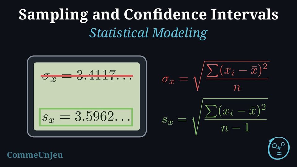
For a list of data, a graphing calculator displays two standard deviations: $\sigma_x$, which divides the sum of the squared deviations by $n$, and $s_x$, which divides it by $n - 1$. The estimate $s_n$ of the population standard deviation is $s_x$, and its square $s_n^2$ is the unbiased estimate of $\sigma^2$. Some formula booklets write this estimate $s_{n-1}$ and keep $s_n$ for the value that divides by $n$; in their notation, the two are linked by $$s_{n-1}^2 = \frac{n}{n-1} \times s_n^2,$$ that is, in the notation of this chapter, $$s_n^2 = \frac{n}{n-1} \times \sigma_x^2.$$ Whatever the notation, the unbiased estimate of $\sigma^2$ divides by $n - 1$. When the data are given in a frequency table, with values $x_i$ and frequencies $f_i$, the sample size is $n = \sum f_i$, the mean is $\bar{x} = \dfrac{\sum f_i x_i}{n}$ and the sum of the squared deviations is $\sum f_i (x_i - \bar{x})^2$.

Report an error

Example — Unbiased Estimates from a Frequency Table

An office worker records the number of e-mails received in each of $40$ randomly chosen hours:

Number of e-mails $x_i$	$0$	$1$	$2$	$3$	$4$	$5$
Frequency $f_i$	$3$	$8$	$12$	$9$	$5$	$3$

Find an unbiased estimate of the mean number $\mu$ of e-mails per hour.
Find an unbiased estimate of the variance $\sigma^2$, by the formula and with a calculator.
The calculator also displays $\sigma_x \approx 1.333$. Explain why $\sigma_x^2$ is not used to estimate $\sigma^2$.

Answer

Here $n = \sum f_i = 40$ and $\sum f_i x_i = 0 + 8 + 24 + 27 + 20 + 15 = 94$, so $$\bar{x} = \frac{\sum f_i x_i}{n} = \frac{94}{40} = 2.35 \text{ e-mails per hour}.$$ The sample mean is an unbiased estimator of $\mu$: the estimate is $2.35$.
The squared deviations are summed with their frequencies: $$\begin{aligned}[t] \sum f_i (x_i - \bar{x})^2 &= \sum f_i x_i^2 - n\bar{x}^2 && \text{(expanding the square)} \\ &= (0 + 8 + 48 + 81 + 80 + 75) - 40 \times 2.35^2 \\ &= 292 - 220.9 = 71.1, \end{aligned}$$ so the unbiased estimate of $\sigma^2$ is $$s_n^2 = \frac{\sum f_i (x_i - \bar{x})^2}{n - 1} = \frac{71.1}{39} \approx 1.82.$$ With a calculator (values in one list, frequencies in another), the one-variable statistics give $s_x \approx 1.3502$, and $s_x^2 \approx 1.82$.
$\sigma_x^2 = \dfrac{71.1}{40} \approx 1.78$ divides by $n$: on average over all samples it underestimates $\sigma^2$. The unbiased estimate divides by $n - 1$, and indeed $\dfrac{40}{39} \times 1.7775 \approx 1.82$.

Skills to practice

Calculating Unbiased Estimates
Modeling with Random Variables
Distinguishing Random Variables and Observed Values

III Normal Combinations and the Central Limit Theorem

III.1 Combining Normal Variables and the Central Limit Theorem

Proposition — Sum and Mean of Normal Variables

If $X_1, \dots, X_n$ are independent and normally distributed with mean $\mu$ and standard deviation $\sigma$, then:

The sum $S_n$ is exactly normally distributed with mean $n\mu$ and variance $n\sigma^2$: $$ S_n \sim N(n\mu, n\sigma^2). $$
The sample mean $\overline{X}_n$ is exactly normally distributed with mean $\mu$ and variance $\dfrac{\sigma^2}{n}$: $$ \overline{X}_n \sim N\!\left(\mu, \frac{\sigma^2}{n}\right). $$

Proposition — Linear Combination of Independent Normal Variables

Let $X_1, \dots, X_n$ be independent random variables with $X_i \sim N(\mu_i, \sigma_i^2)$, and let $a_1, \dots, a_n$ be constants, not all zero. Then the linear combination $Y = a_1 X_1 + \dots + a_n X_n$ is normally distributed: $$Y \sim N\!\left(a_1\mu_1 + \dots + a_n\mu_n,\ a_1^2\sigma_1^2 + \dots + a_n^2\sigma_n^2\right).$$ The mean and the variance come from the Proposition “Properties of Expectation and Variance”; that $Y$ is again normal is admitted. In particular:

for two independent normal variables, $X - Y \sim N\!\left(\mu_X - \mu_Y,\ \sigma_X^2 + \sigma_Y^2\right)$: the variances add;
for independent variables with the same distribution $N(\mu, \sigma^2)$, the sum and the mean give the Proposition “Sum and Mean of Normal Variables”.

To compare two normal quantities, the event is written with their difference: $P(X > Y) = P(X - Y > 0)$.

Example

Let $X_1, \dots, X_5$ be normally distributed random variables with mean $90$ and standard deviation $20$.

Is $\overline{X}_5$ normally distributed?
Find $P(80 \leq \overline{X}_5 \leq 100)$.

Answer

Yes, because any linear combination of independent normal variables is also normal. In particular, the mean $\overline{X}_5$ is normally distributed.
The mean of $\overline{X}_5$ is $E(\overline{X}_5) = 90$. Its standard deviation is $$ \sigma(\overline{X}_5) = \frac{20}{\sqrt{5}} \approx 8.94. $$ Using a normal distribution calculator for $N(90, 8.94^2)$, we obtain $$P(80 \leq \overline{X}_5 \leq 100) \approx 0.736.$$

Example

In a bakery, the mass of a large loaf follows $L \sim N(820, 15^2)$ and the mass of a small loaf $S \sim N(400, 10^2)$, in grams; the masses of different loaves are independent.

One large loaf and one small loaf are chosen at random. Find the probability that the large loaf weighs more than twice the small loaf.
One large loaf and two small loaves are chosen at random. Find the probability that the large loaf weighs more than the two small loaves together.

Round the probabilities to three significant figures.

Answer

The event is $L > 2S$, that is $D > 0$ with $D = L - 2S$, a linear combination of the independent normal variables $L$ and $S$ (coefficients $1$ and $-2$): $$\begin{aligned}[t] E(D) &= E(L) - 2E(S) = 820 - 2 \times 400 = 20, \\ V(D) &= V(L) + (-2)^2 V(S) && \text{(independent variables)} \\ &= 15^2 + 4 \times 10^2 = 625, \end{aligned}$$ so $D \sim N(20, 25^2)$ and, with the normal cumulative function, $P(L > 2S) = P(D > 0) \approx 0.788$.
With two independent small loaves $S_1$ and $S_2$, let $D' = L - S_1 - S_2$ (coefficients $1$, $-1$, $-1$): $$\begin{aligned}[t] E(D') &= 820 - 400 - 400 = 20, \\ V(D') &= 15^2 + 10^2 + 10^2 = 425, \end{aligned}$$ so $D' \sim N(20, 425)$, $\sigma(D') = \sqrt{425} \approx 20.62$, and $P(D' > 0) \approx 0.834$.

The two differences have the same mean, but $2S$ has variance $4 \times 10^2 = 400$ while $S_1 + S_2$ has variance $200$: doubling one small loaf is not the same as putting two small loaves together.

Example

A cable car carries $6$ adults and $4$ children. The mass of an adult is modelled by $N(78, 12^2)$ and the mass of a child by $N(35, 8^2)$, in kilograms, all the masses being independent. The maximum load of the cabin is $650$ kg.

Find the mean and the standard deviation of the total mass $M$ of the passengers.
Find the probability that the maximum load is exceeded, to three significant figures.
State an assumption of the model that may fail in practice.

Answer

$M = A_1 + \dots + A_6 + C_1 + \dots + C_4$ is the sum of ten independent normal variables: $$\begin{aligned}[t] E(M) &= 6 \times 78 + 4 \times 35 = 608, \\ V(M) &= 6 \times 12^2 + 4 \times 8^2 && \text{(independent variables)} \\ &= 864 + 256 = 1120, \end{aligned}$$ so $\sigma(M) = \sqrt{1120} \approx 33.47$ kg.
By the Proposition “Linear Combination of Independent Normal Variables”, $M \sim N(608, 1120)$, and the normal cumulative function gives $$P(M > 650) \approx 0.105$$ ($z = \dfrac{650 - 608}{\sqrt{1120}} \approx 1.255$).
The masses are assumed independent. The passengers of one cabin are often a family or a group, whose masses are related (children travel with their parents); the adults of one cabin are not a random sample either.

The Central Limit Theorem (CLT) is one of the most remarkable results in mathematics. Informally, it states that if you take a sufficiently large sample size from a population with any distribution (not necessarily normal), the distribution of the sample mean (or sum) is approximately normal.
This normal approximation is what justifies using the normal distribution to build confidence intervals and perform hypothesis tests, even when the underlying population is not itself normal.

Report an error

Proposition — Standardized Mean

For $n$ independent random variables with common mean $\mu$ and standard deviation $\sigma$, the sample mean $\overline{X}_n$ has$$ E(\overline{X}_n) = \mu, \qquad \sigma(\overline{X}_n) = \frac{\sigma}{\sqrt{n}}. $$ The standardized variable$$ Z_n = \frac{\overline{X}_n - \mu}{\sigma/\sqrt{n}} $$ has mean $0$ and standard deviation $1$.

Proof

First, recall the properties of the sample mean $\overline{X}_n$:$$ E(\overline{X}_n) = \mu \quad \text{and} \quad \sigma(\overline{X}_n) = \frac{\sigma}{\sqrt{n}}. $$

Mean of $Z_n$:
Using linearity of expectation, $E(aX+b) = aE(X)+b$:$$ \begin{aligned}E(Z_n) &= E\left(\frac{\overline{X}_n - \mu}{\sigma/\sqrt{n}}\right) \\ &= \frac{1}{\sigma/\sqrt{n}} \left( E(\overline{X}_n) - \mu \right) \\ &= \frac{1}{\sigma/\sqrt{n}} (\mu - \mu) \\ &= 0.\end{aligned} $$
Standard deviation of $Z_n$:
Using the property $\sigma(aX+b) = |a|\sigma(X)$:$$ \begin{aligned}\sigma(Z_n) &= \sigma\left(\frac{\overline{X}_n - \mu}{\sigma/\sqrt{n}}\right) \\ &= \frac{1}{\sigma/\sqrt{n}} \cdot \sigma(\overline{X}_n) \\ &= \frac{1}{\sigma/\sqrt{n}} \cdot \frac{\sigma}{\sqrt{n}} \\ &= 1.\end{aligned} $$

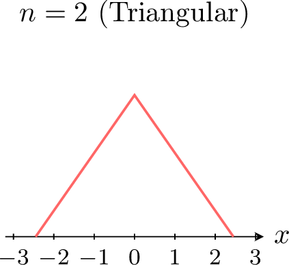
The power of the Central Limit Theorem is especially visible when we start from a distribution that is not normal. For example, suppose each $X_i$ follows a uniform distribution. The figures below show the density of the standardized sum (or mean) $Z_n$ for increasing $n$.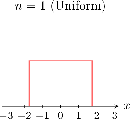

$\quad$

$\quad$

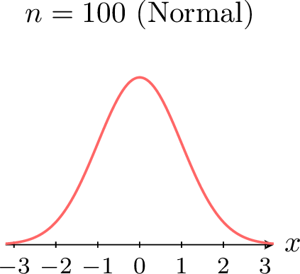
When $n=1$, we see a flat rectangular density (uniform distribution). For $n=2$, the density becomes triangular. For large $n$ (for example $n=100$), the curve is visually indistinguishable from the bell curve of a standard normal distribution.

Report an error

Theorem — Central Limit Theorem

Let $X_1, X_2, \dots, X_n$ be independent, identically distributed random variables with mean $\mu$ and standard deviation $\sigma$. If the sample size $n$ is sufficiently large (typically $n \ge 30$), then:

The sample mean $\overline{X}_n$ is approximately normally distributed: $$ \overline{X}_n \approx N\!\left(\mu, \frac{\sigma^2}{n}\right). $$
The sum $S_n$ is approximately normally distributed: $$ S_n \approx N(n\mu, n\sigma^2). $$
The standardized variable $$ Z_n = \frac{\overline{X}_n - \mu}{\sigma/\sqrt{n}} $$ is approximately distributed as a standard normal $N(0,1)$ for large $n$. More rigorously, the distribution of $Z_n$ converges to $N(0,1)$ as $n \to \infty$.

Example

A population of random variables has mean $174$ and standard deviation $6$. A sample of size $64$ is taken.

Is the sample mean $\overline{X}_{64}$ approximately normally distributed? Explain.
Find the mean and standard deviation of $\overline{X}_{64}$.
Find the probability that the sample mean is between $172$ and $176$.

Answer

Yes. Since the sample size is $n=64$ (which is large, $n \ge 30$), the Central Limit Theorem applies, and the sampling distribution of $\overline{X}_{64}$ is approximately normal.
Mean and standard deviation: $$ E(\overline{X}_{64}) = \mu = 174, $$ $$ \sigma(\overline{X}_{64}) = \frac{\sigma}{\sqrt{n}} = \frac{6}{\sqrt{64}} = \frac{6}{8} = 0.75. $$
Using a normal distribution calculator with $\mu=174$ and $\sigma=0.75$: $$ P(172 \leq \overline{X}_{64} \leq 176) \approx 0.9923. $$

Skills to practice

Combining Normal Variables
Analyzing the Sum of Normal Variables
Comparing Two Normal Quantities
Applying the Central Limit Theorem
Calculating Quantiles Using the Normal Approximation

IV Confidence Intervals for a Mean

IV.1 Known Standard Deviation

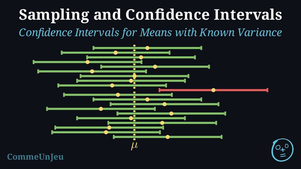
A point estimate, like the sample mean $\bar{x}$, provides a single value as an estimate of the population parameter. However, it does not tell us how precise this estimate is. Due to sampling variability, $\bar{x}$ is rarely exactly equal to the true mean $\mu$.
To address this, we use a confidence interval. A confidence interval provides a range of values within which we expect the true population parameter to lie, with a certain level of confidence. Suppose the population variance $\sigma^2$ is known, which allows us to use the standard normal distribution ($Z$).

Report an error

Proposition — Probability Interval

Assume we take a sample of size $n$ from a population with mean $\mu$ and standard deviation $\sigma$, and that $n$ is sufficiently large (typically $n \ge 30$ so that the Central Limit Theorem applies). Then$$ P\left(\overline{X}_n - 1.96 \frac{\sigma}{\sqrt{n}} \leq \mu \leq \overline{X}_n + 1.96 \frac{\sigma}{\sqrt{n}}\right) = 0.95. $$

Proof

Since $n$ is large, the Central Limit Theorem applies. The sampling distribution of the mean $\overline{X}_n$ is approximately normal with mean $\mu$ and standard deviation $\dfrac{\sigma}{\sqrt{n}}$.
The standardized variable $Z$ follows a standard normal distribution:$$ Z = \frac{\overline{X}_n - \mu}{\sigma/\sqrt{n}} \sim N(0, 1). $$ For a $95\pourcent$ confidence level, we seek the critical value $z$ such that $P(-z \leq Z \leq z) = 0.95$.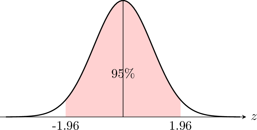

Using a calculator (Inverse Normal), we find $z \approx 1.96$.$$\begin{aligned}P\left(-1.96 \leq \frac{\overline{X}_n - \mu}{\sigma/\sqrt{n}} \leq 1.96\right) &= 0.95 \\ P\left(-1.96 \frac{\sigma}{\sqrt{n}} \leq \overline{X}_n - \mu \leq 1.96 \frac{\sigma}{\sqrt{n}}\right) &= 0.95 \\ P\left(\overline{X}_n - 1.96 \frac{\sigma}{\sqrt{n}} \leq \mu \leq \overline{X}_n + 1.96 \frac{\sigma}{\sqrt{n}}\right) &= 0.95.\end{aligned}$$ This is the stated probability interval.

The proposition above gives us a probability statement about the random sample mean $\overline{X}_n$ and the random interval built from it. The parameter $\mu$ is fixed (but unknown); what is random is the interval itself.
To calculate a specific confidence interval in practice, we estimate this probability interval by replacing the random variable $\overline{X}_n$ with the observed sample mean $\bar{x}$. Thus, the confidence interval we compute is an estimate of the theoretical interval.

Report an error

Method — Calculating the Confidence Interval (Mean)

Identify the statistics: Find the sample mean $\bar{x}$, the known population standard deviation $\sigma$, and the sample size $n$.
Find the z-score: Determine $z$ based on the confidence level (1.645 for 90$\pourcent$, 1.96 for 95$\pourcent$, 2.576 for 99$\pourcent$).
Calculate the margin of error: $E = z \dfrac{\sigma}{\sqrt{n}}$.
Write the interval: $[\bar{x} - E, \bar{x} + E]$.

Example

A sample of 60 rabbits was taken from a forest. The sample mean weight of the rabbits was $950$ grams. Assume the population standard deviation is known to be $\sigma = 200$ grams.
Find the $95\pourcent$ confidence interval for the population mean weight.

Answer

Statistics: $n=60$, $\bar{x}=950$, and $\sigma=200$.
z-score: For $95\pourcent$, $z = 1.96$.
Margin of error: $$ E = 1.96 \times \frac{200}{\sqrt{60}} \approx 1.96 \times 25.82 \approx 50.6. $$
Interval: $$ [950 - 50.6, \ 950 + 50.6] = [899.4, 1000.6]. $$

We are 95$\pourcent$ confident that the true mean weight is between 899.4g and 1000.6g.

Skills to practice

Finding Critical Values
Computing Confidence Intervals with a Known Standard Deviation
Constructing Confidence Intervals

IV.2 Unknown Standard Deviation

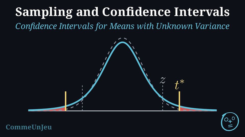
In most practical situations, the population standard deviation $\sigma$ is unknown. We cannot use the normal distribution ($Z$) with a known $\sigma$, because we must estimate $\sigma$ using the sample standard deviation $s_n$.
In theory, when the population is normal and $\sigma$ is unknown, the exact sampling distribution of$$ \frac{\overline{X}_n - \mu}{S_n/\sqrt{n}} $$ is a Student's t-distribution with $n-1$ degrees of freedom. For large samples (say $n \ge 30$), the t-distribution is very close to the standard normal distribution. For large $n$, the same $z$-values are used, with $\sigma$ replaced by $s_n$. The $t$-distribution is exact at every sample size, small or large, when the population is normal; for a population far from normal, only a large sample gives an interval, built with $t$ or with $z$, and this interval is approximate.

Report an error

Definition — The t-Distribution

Let $\overline{X}_n$ be the mean and $S_n^2$ the unbiased variance estimator of a random sample of size $n$ taken from a normal population of mean $\mu$. The random variable $$T = \frac{\overline{X}_n - \mu}{S_n / \sqrt{n}}$$ follows the $t$-distribution (Student's distribution) with $n - 1$ degrees of freedom; we write $T \sim t_{n-1}$. Its density curve is bell-shaped and symmetric about $0$, like that of $\mathcal{N}(0, 1)$, but lower in the middle and with heavier tails: estimating $\sigma$ by $S_n$ adds variability. The larger the number of degrees of freedom, the closer the $t$-distribution is to $\mathcal{N}(0, 1)$.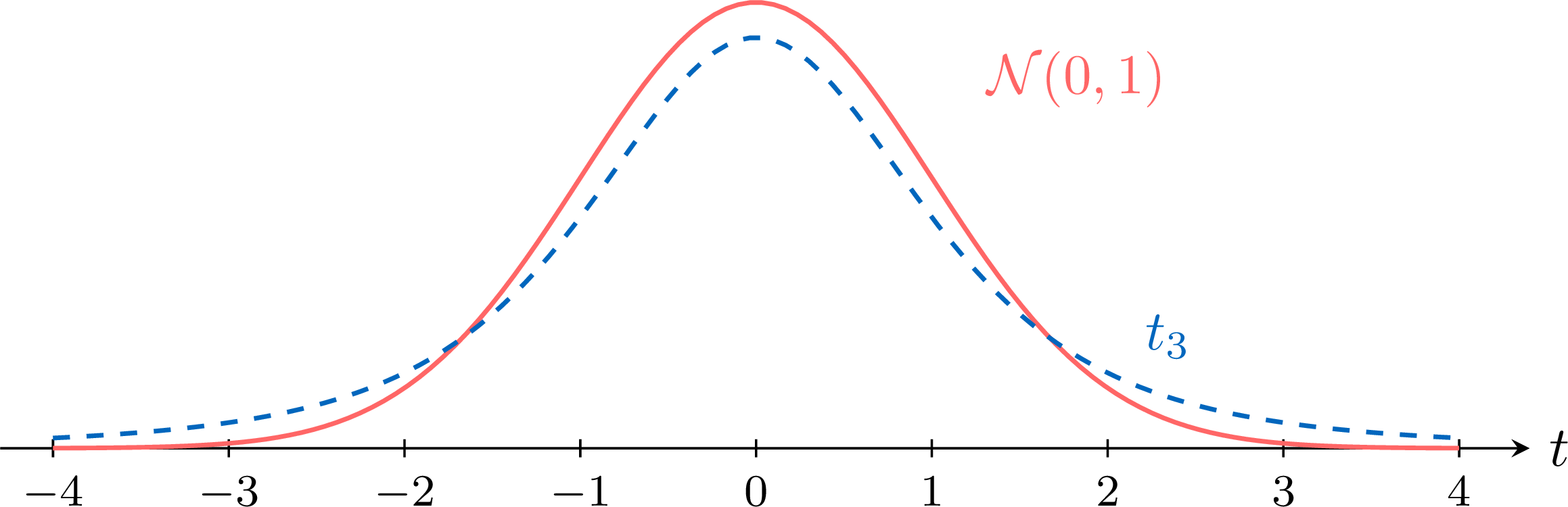

Method — Confidence Interval for a Mean When the Standard Deviation Is Unknown

When $\sigma$ is unknown, the interval is built with $t$, whatever the size of the sample.

Check the conditions: a random sample, $\sigma$ unknown, and a population that is approximately normal or a large sample (commonly $n \geq 30$, more when the population is strongly skewed).
Compute the statistics: $n$, $\bar{x}$ and $s_n$ (the key $s_x$ of a calculator, which divides by $n - 1$).
Find the critical value: for a confidence level $1 - \alpha$, the number $t^*$ such that $P(-t^* \leq T \leq t^*) = 1 - \alpha$ with $T \sim t_{n-1}$, that is $P(T \leq t^*) = 1 - \dfrac{\alpha}{2}$. The inverse $t$ function of a calculator (InvT) gives it from the area $1 - \dfrac{\alpha}{2}$ and the $n - 1$ degrees of freedom; for $95\pourcent$ and $n = 10$, $t^* \approx 2.262$ (against $1.960$ for $z$).
Compute the margin of error: $E = t^* \dfrac{s_n}{\sqrt{n}}$.
Write the interval: $[\bar{x} - E, \bar{x} + E]$, then interpret it in context. The method produces intervals that contain $\mu$ for a proportion $1 - \alpha$ of the samples (exactly for a normal population, approximately otherwise); the parameter $\mu$ is fixed, the interval is what varies.

The T-interval function of a calculator (TInterval) carries out steps 2 to 4 at once, from the list of the data or from $\bar{x}$, $s_n$ and $n$; its sister, the Z-interval function, does the same when $\sigma$ is known. Round only at the end. The mock-ups show the data of the next example: $n = 10$, $\bar{x} = 1002.6$, $s_n \approx 5.758$.

Example

A machine fills bags of rice labelled $1$ kg. The masses, in grams, of $10$ bags chosen at random are $$1004, \ 996, \ 1011, \ 998, \ 1007, \ 1002, \ 993, \ 1009, \ 1001, \ 1005.$$ The masses are assumed to be normally distributed.

Find a $95\pourcent$ confidence interval for the mean mass $\mu$ of the bags filled by the machine.
Interpret the interval in context.

Answer

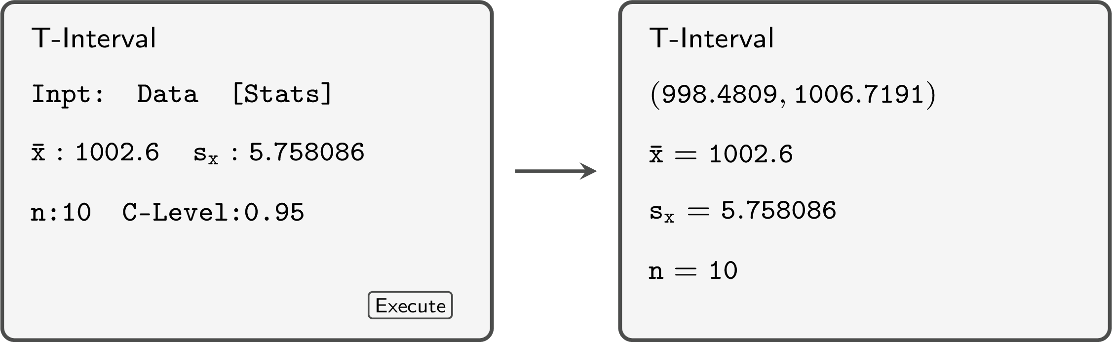
The population is normal and $\sigma$ is unknown: $t$-interval with $n - 1 = 9$ degrees of freedom. With a calculator, $\bar{x} = 1002.6$ and $s_n \approx 5.7581$; InvT$(0.975, 9)$ gives $t^* \approx 2.2622$. Then $$\begin{aligned}[t] E &= t^* \frac{s_n}{\sqrt{n}} && \text{(margin of error)} \\ &\approx 2.2622 \times \frac{5.7581}{\sqrt{10}} \approx 4.119, \end{aligned}$$ and the interval is $[1002.6 - 4.119, \ 1002.6 + 4.119] \approx [998.48, 1006.72]$ g, as the T-interval function gives.
We are $95\pourcent$ confident that the mean mass of the bags filled by the machine lies between $998.48$ g and $1006.72$ g: this method gives an interval containing $\mu$ for $95\pourcent$ of samples. The labelled $1000$ g lies inside the interval.

Method — Calculating the Confidence Interval (Unknown $\sigma$, Large $n$)

Identify the statistics: Find the sample mean $\bar{x}$, the sample standard deviation $s_n$ (as an estimate for $\sigma$), and the sample size $n$.
Find the z-score: Determine $z$ based on the confidence level (1.645 for 90$\pourcent$, 1.96 for 95$\pourcent$, 2.576 for 99$\pourcent$), provided $n$ is large.
Calculate the margin of error: $E = z \dfrac{s_n}{\sqrt{n}}$.
Write the interval: $[\bar{x} - E, \bar{x} + E]$.

Example

An economist studying fuel costs wants to estimate the mean price of gasoline in her state. She takes a random sample of 40 gas stations and finds a sample mean price of $\bar{x} = \dollar 1.29$ with a sample standard deviation of $s_n = \dollar 0.10$.
Find the $95\pourcent$ confidence interval for the population mean.

Answer

Statistics: $n=40$, $\bar{x}=1.29$, and $s_n=0.10$. (Since $n \ge 30$, we approximate $\sigma \approx s_n$.)
z-score: For $95\pourcent$, $z = 1.96$.
Margin of error: $$ E = 1.96 \times \frac{0.10}{\sqrt{40}} \approx 1.96 \times 0.0158 \approx 0.031. $$
Interval: $$ [1.29 - 0.031, \ 1.29 + 0.031] = [1.259, 1.321]. $$

We are 95$\pourcent$ confident that the true mean price is between $\dollar 1.259$ and $\dollar 1.321$.

Example

The waiting times at a hospital reception are not normally distributed: their distribution is moderately skewed, most waits being short and a few longer. For a random sample of $50$ patients, the mean waiting time is $\bar{x} = 12.6$ minutes and $s_n = 4.8$ minutes.

Explain why a confidence interval for the mean waiting time $\mu$ can still be built.
Find the $95\pourcent$ $t$-interval for $\mu$.
Find the interval obtained with $z = 1.96$ in place of $t^*$, and compare.

Answer

The sample is large ($n = 50 \geq 30$) and the skew is only moderate: by the central limit theorem, $\overline{X}_n$ is approximately normal, so the interval is valid, but only approximately, since the population is not normal.
With $49$ degrees of freedom, $t^* \approx 2.0096$, so $$E = t^* \frac{s_n}{\sqrt{n}} \approx 2.0096 \times \frac{4.8}{\sqrt{50}} \approx 1.364,$$ and the interval is approximately $[11.24, 13.96]$ minutes.
With $z = 1.96$: $E \approx 1.96 \times \dfrac{4.8}{\sqrt{50}} \approx 1.330$, and the interval is approximately $[11.27, 13.93]$ minutes. For $n = 50$, $t^*$ and $z$ differ by about $0.05$: the two intervals agree to within a few hundredths of a minute, the $t$-interval being a little wider. This is why the $z$-interval with $s_n$ (Method “Calculating the Confidence Interval (Unknown $\sigma$, Large $n$)”) is a good approximation for large samples; the $t$-interval remains the method used when $\sigma$ is unknown.

Skills to practice

Finding Critical Values of t
Computing t-Intervals
Estimating a Mean with a t-Interval

V Going further

Skills to practice

Diagnosing and Correcting
Solving Problems
Quiz

\(s\) (Sum)	\(0\)	\(1\)	\(2\)
\(P(S_2=s)\)	\(1/4\)	\(1/2\)	\(1/4\)

\(\bar{x}\) (Mean)	\(0\)	\(0.5\)	\(1\)
\(P(\overline{X}_2=\bar{x})\)	\(1/4\)	\(1/2\)	\(1/4\)

Number of e-mails \(x_i\)	\(0\)	\(1\)	\(2\)	\(3\)	\(4\)	\(5\)
Frequency \(f_i\)	\(3\)	\(8\)	\(12\)	\(9\)	\(5\)	\(3\)