International Baccalaureate · DP 1: Applications and Interpretation HL
Conditional Probability
I
Two-Way Tables
I.1
Counts and Frequencies
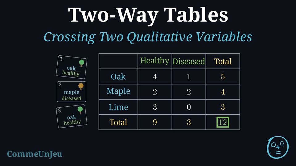
A data file describes individuals — people, animals, towns, cars — by several characteristics: species, region, profession, level of satisfaction. Crossing two of these characteristics in one table answers questions that a single list cannot: do the members of one group behave like those of another? which group holds most of a given category? A two-way table of counts is the first tool of data analysis, and reading it carefully is what keeps a sentence such as “most of the accidents with injuries happen in town” from being confused with “an accident in town is more often a serious one”.
Definition — Qualitative Variable
A qualitative variable describes the individuals of a population by a category, not by a number. Its possible values are its categories. The variable is nominal when the categories have no natural order (species, profession, region of residence) and ordinal when they do (level of education, degree of satisfaction, age group). Definition — Two-Way Table of Counts
Two qualitative variables are observed on the same population of \(N\) individuals. The two-way table of counts has one row for each category of the first variable and one column for each category of the second; the cell at row \(A\) and column \(B\) holds the count of the individuals that have both categories \(A\) and \(B\), written \(n(A \cap B)\). - The last column holds the row totals: \(n(A)\) is the number of individuals of category \(A\).
- The last row holds the column totals: \(n(B)\) is the number of individuals of category \(B\).
- The bottom-right cell holds the grand total \(N\), which is the sum of the row totals and the sum of the column totals.
Definition — Marginal Frequency
In a two-way table with grand total \(N\), the row and column totals are the marginal counts: they are read in the margins of the table. The marginal frequency of a category \(A\) is the proportion of the whole population that has this category: $$\textcolor{colordef}{f(A) = \frac{n(A)}{N}}.$$ Here the word frequency denotes a proportion, the relative frequency; a number of individuals is a count. Likewise the frequency of a cell is \(\dfrac{n(A \cap B)}{N}\), the proportion of the whole population that has both categories. The marginal frequencies of the categories of one variable add up to \(1\), that is \(100\pourcent\). Example
The \(200\) members of a sports club are sorted by gender and by the sport they practise: | Swimming | Athletics | Total | |
| Women | \(72\) | \(48\) | \(120\) |
| Men | \(32\) | \(48\) | \(80\) |
| Total | \(104\) | \(96\) | \(200\) |
The marginal counts are the totals of the rows and of the columns; each is divided by \(N = 200\): $$\begin{aligned} f(\text{Women}) &= \frac{120}{200} = 0.6, & f(\text{Men}) &= \frac{80}{200} = 0.4, \\
f(\text{Swimming}) &= \frac{104}{200} = 0.52, & f(\text{Athletics}) &= \frac{96}{200} = 0.48. \end{aligned}$$ Check: \(0.6 + 0.4 = 1\) and \(0.52 + 0.48 = 1\). Women are \(60\pourcent\) of the club, and swimming is the sport of \(52\pourcent\) of the members.
Definition — Conditional Frequency
The conditional frequency of a category \(B\) given a category \(A\) observed at least once (\(n(A) > 0\)) is the proportion of the individuals of \(A\) that also have \(B\): $$\textcolor{colordef}{f_A(B) = \frac{n(A \cap B)}{n(A)}}.$$ It is computed inside the sub-population \(A\): the numerator is the cell at row \(A\) and column \(B\), the denominator is the marginal count of \(A\), not the grand total. The conditional frequencies given \(A\) of all the categories of the other variable add up to \(1\). Method — Row Profiles and Column Profiles
To compare the groups defined by one variable: - Choose the variable that defines the groups: its categories are the rows (or the columns) of the table.
- Divide each cell of a row by the total of that row (a row observed at least once): the row now reads as conditional frequencies, its row profile — the list of the \(f_A(B)\) for the category \(A\) of that row — which adds up to \(1\).
- Compare the profiles row by row: two groups with the same profile are distributed alike over the other variable.
Example
In the sports club of \(200\) members (women \(72\) swimmers and \(48\) athletes, men \(32\) swimmers and \(48\) athletes): - Compute the frequency of swimming among the women and among the men. Do the two groups practise the same sports in the same proportions?
- Compute the frequency of women among the swimmers and among the athletes.
- The groups are the rows. Each cell is divided by its row total: $$\begin{aligned} f_{\text{Women}}(\text{Swimming}) &= \frac{n(\text{Women} \cap \text{Swimming})}{n(\text{Women})} = \frac{72}{120} = 0.6, \\ f_{\text{Men}}(\text{Swimming}) &= \frac{n(\text{Men} \cap \text{Swimming})}{n(\text{Men})} = \frac{32}{80} = 0.4. \end{aligned}$$ The row profiles are \((0.6\,;\,0.4)\) for the women and \((0.4\,;\,0.6)\) for the men: \(60\pourcent\) of the women swim, against \(40\pourcent\) of the men. The two groups do not practise the sports in the same proportions.
- The groups are now the columns. Each cell is divided by its column total: $$\begin{aligned} f_{\text{Swimming}}(\text{Women}) &= \frac{72}{104} = \frac{9}{13} \approx 0.69, \\ f_{\text{Athletics}}(\text{Women}) &= \frac{48}{96} = 0.5. \end{aligned}$$ About \(69\pourcent\) of the swimmers are women, and exactly half of the athletes. Note that \(f_{\text{Women}}(\text{Swimming}) = 0.6\) and \(f_{\text{Swimming}}(\text{Women}) \approx 0.69\) share the numerator \(72\) but not the denominator: “\(60\pourcent\) of the women swim” and “\(69\pourcent\) of the swimmers are women” are two different facts.
Reading a Sentence
A sentence about a two-way table names a frequency, and the words tell which one. “\(60\pourcent\) of the women swim”: the population is restricted to the women, then the swimmers are counted among them — a conditional frequency, \(f_{\text{Women}}(\text{Swimming})\). “\(36\pourcent\) of the members are women who swim”: the population is the whole club and the category is “woman and swimmer” — the frequency of a cell, \(\frac{72}{200}\). “\(52\pourcent\) of the members swim”: a marginal frequency, \(f(\text{Swimming})\). The words of the, among, out of introduce the group that serves as the denominator. Many sentences in the media are true and yet misread, because the reader takes a column profile for a row profile: “most of the swimmers are women” does not mean that most women swim. In a club where \(40\) of the \(100\) women and \(10\) of the \(100\) men swim, \(80\pourcent\) of the swimmers are women, while only \(40\pourcent\) of the women swim.
Skills to practice
- Computing Conditional Frequencies
I.2
Completing a Two-Way Table
Method — Completing by Reasoning on the Counts
Every row total is the sum of the cells of its row, every column total is the sum of the cells of its column, and the grand total is the sum of the row totals as well as the sum of the column totals. To fill in a missing cell: - Find a line (row or column) where only one number is missing.
- Subtract the known cells from the total of that line, or add the cells if the total is the missing number.
- Repeat with the lines that are now complete but one.
- Check that the row totals and the column totals both add up to the grand total.
Method — Completing with Conditional Frequencies
A frequency given in words is turned back into a count by multiplying it by the size of the group it refers to: - a marginal frequency gives a marginal count: \(n(A) = f(A) \times N\);
- a conditional frequency gives a cell: \(n(A \cap B) = f_A(B) \times n(A)\) — the group is \(A\), the one after “of the” or “among”.
Example
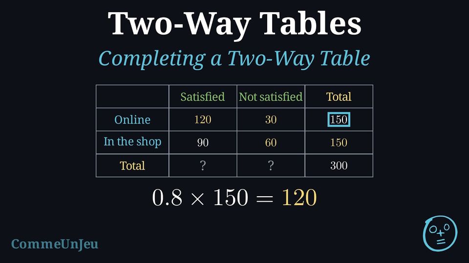
A shop surveys \(300\) customers about their satisfaction, each customer being classified by the channel of their last purchase, online or in the shop. \(150\) of them bought online, and \(80\pourcent\) of the online customers are satisfied. Among the customers who bought in the shop, \(90\) are satisfied. Complete the two-way table of counts and compute the marginal frequency of the satisfied customers.
“\(80\pourcent\) of the online customers” is a conditional frequency given the group “online”, of size \(150\): \(n(\text{online} \cap \text{satisfied}) = 0.8 \times 150 = 120\). The rest follows by subtraction: online not satisfied \(150 - 120 = 30\); in the shop \(300 - 150 = 150\) customers, of whom \(90\) satisfied and \(150 - 90 = 60\) not satisfied.
Check: \(210 + 90 = 300\). The marginal frequency of the satisfied customers is \(f(\text{Satisfied}) = \frac{210}{300} = 0.7\): \(70\pourcent\) of the customers are satisfied, a figure that lies between the \(80\pourcent\) of the online customers and the \(60\pourcent\) of the shop customers.
| Satisfied | Not satisfied | Total | |
| Online | \(120\) | \(30\) | \(150\) |
| In the shop | \(90\) | \(60\) | \(150\) |
| Total | \(210\) | \(90\) | \(300\) |
Skills to practice
- Completing by Reasoning on the Counts
- Completing with Conditional Frequencies
II
Conditional Probability
II.1
Definition
Conditional probability can be explored with a two-way table showing the preferences of 100 students for maths, split by gender:
A student is picked at random, all students being equally likely. Some probabilities follow from the table:
| Loves Maths | Does Not Love Maths | Total | |
| Girls | 35 | 16 | 51 |
| Boys | 30 | 19 | 49 |
| Total | 65 | 35 | 100 |
- Probability the student is a girl: $$\begin{aligned} P(\text{Girl}) &= \frac{\text{Number of girls}}{\text{Number of students}} \\ &= \frac{51}{100}. \end{aligned}$$
- Probability the student loves maths and is a girl: $$\begin{aligned} P(\text{Loves Maths and Girl}) &= \frac{\text{Number of girls who love maths}}{\text{Number of students}} \\ &= \frac{35}{100}. \end{aligned}$$
- Probability the student loves maths, given they are a girl:
Since the student is known to be a girl, only the 51 girls count: $$\begin{aligned} \PCond{\text{Loves Maths}}{\text{Girl}} &= \frac{\text{Number of girls who love maths}}{\text{Number of girls}} \\ &= \frac{35}{51}. \end{aligned}$$ - Connecting to the formula:
Notice that: $$\begin{aligned} \PCond{\text{Loves Maths}}{\text{Girl}} &=\frac{35}{51}\\ &= \frac{35/100}{51/100}\\ &= \dfrac{P(\text{Loves Maths and Girl})}{P(\text{Girl})}. \end{aligned}$$ This pattern gives the general rule for conditional probability.
Definition — Conditional Probability
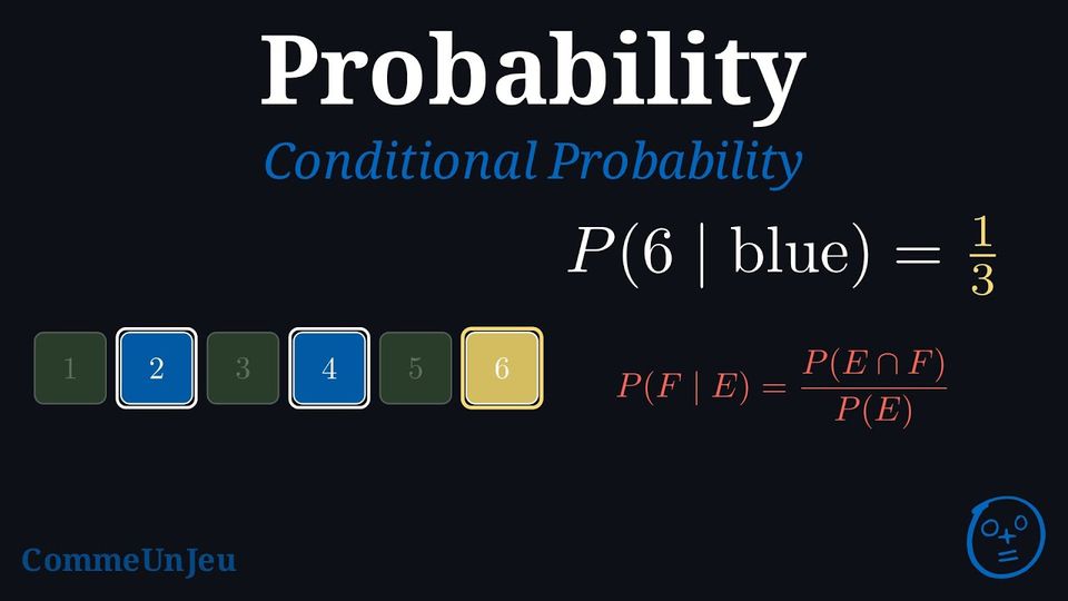
The conditional probability of event \(F\) given event \(E\) is the probability of \(F\) occurring, given that \(E\) occurs. It’s denoted \(\PCond{F}{E}\) and calculated as: $$\textcolor{colordef}{\PCond{F}{E} = \frac{P(E \cap F)}{P(E)}}, \quad \text{where } P(E) > 0.$$
Two Notations
There are two notations for the conditional probability of \(F\) given \(E\). French textbooks write \(P_E(F)\), with the known event \(E\) as an index; international textbooks write \(\PCond{F}{E}\), with the known event after a bar. They name the same number: $$P_E(F) = \PCond{F}{E} = \frac{P(E \cap F)}{P(E)}.$$ In both, \(F\) is the event whose probability is computed and \(E\) is the information already known. In the two-way table of the \(100\) students, \(35\) of the \(51\) girls love maths: \(P_{\text{Girl}}(\text{Loves Maths}) = \PCond{\text{Loves Maths}}{\text{Girl}} = \frac{35}{51}\).
Proposition — Conditional Probability and Counts
An individual is chosen at random, all individuals being equally likely, in a population \(U\) of \(\Card{U}\) individuals. For two events \(A\) and \(B\), with \(B\) containing at least one individual: $$\textcolor{colorprop}{P(A) = \frac{\Card{A}}{\Card{U}}} \qquad \text{and} \qquad \textcolor{colorprop}{\PCond{A}{B} = \frac{\Card{A \cap B}}{\Card{B}}}.$$ Here \(\Card{A}\) is the number of elements of \(A\). The conditional probability of \(A\) given \(B\) is the proportion of the individuals of \(B\) that are also in \(A\): the known event \(B\) becomes the new population.
By the Definition “Equally Likely”, \(P(A) = \dfrac{\Card{A}}{\Card{U}}\) and \(P(B) = \dfrac{\Card{B}}{\Card{U}}\). Then: $$\begin{aligned} \PCond{A}{B} &= \frac{P(A \cap B)}{P(B)} && \text{(Definition ``Conditional Probability'')} \\
&= \frac{\Card{A \cap B}/\Card{U}}{\Card{B}/\Card{U}} && \text{(Definition ``Equally Likely'')} \\
&= \frac{\Card{A \cap B}}{\Card{U}} \times \frac{\Card{U}}{\Card{B}} && \text{(dividing by a fraction)} \\
&= \frac{\Card{A \cap B}}{\Card{B}}. \end{aligned}$$
Proposition — Conditioning Changes the Probability, Not the Events
Let \(E\) be an event with \(P(E) > 0\). Taking each event \(F\) of the sample space \(U\) to the number \(\PCond{F}{E}\) defines a new probability on the same sample space: \(\PCond{F}{E} \geq 0\) for every event \(F\); \(\PCond{U}{E} = 1\); and if \(F \cap G = \emptyset\), then \(\PCond{F \cup G}{E} = \PCond{F}{E} + \PCond{G}{E}\). The events are the same subsets of \(U\) as before; only the numbers attached to them change. The new probability gives \(1\) to \(E\) and \(0\) to \(E'\), although \(E'\) is not empty when \(E \neq U\). Every rule proved for a probability therefore holds for it: for instance \(\PCond{F'}{E} = 1 - \PCond{F}{E}\), which is why the probabilities on the branches leaving one node of a tree add up to \(1\).
The three properties are the axioms of a probability, checked for the numbers \(\PCond{F}{E}\).
- Each \(\PCond{F}{E} = \dfrac{P(E \cap F)}{P(E)}\) is the quotient of \(P(E \cap F) \geq 0\) (Axiom 1) by \(P(E) > 0\), so \(\PCond{F}{E} \geq 0\).
- \(E \cap U = E\), so \(\PCond{U}{E} = \dfrac{P(E \cap U)}{P(E)} = \dfrac{P(E)}{P(E)} = 1\). In the same way, \(E \cap E = E\) gives \(\PCond{E}{E} = 1\).
- Let \(F\) and \(G\) be events with \(F \cap G = \emptyset\). The events \(E \cap F\) and \(E \cap G\) have no outcome in common, since a common outcome would lie in \(F \cap G\): they are mutually exclusive. Their union is \(E \cap (F \cup G)\): an outcome of \(E\) lies in \(F \cup G\) exactly when it lies in \(F\) or in \(G\). So $$\begin{aligned}[t] \PCond{F \cup G}{E} &= \frac{P\big(E \cap (F \cup G)\big)}{P(E)} && \text{(Definition ``Conditional Probability'')}\\ &= \frac{P\big((E \cap F) \cup (E \cap G)\big)}{P(E)} && \text{(distributivity of \(\cap\) over \(\cup\))}\\ &= \frac{P(E \cap F) + P(E \cap G)}{P(E)} && \text{(Axiom 3)}\\ &= \PCond{F}{E} + \PCond{G}{E}. \end{aligned}$$
- Finally \(E \cap E' = \emptyset\), and \(P(\emptyset) = 1 - P(U) = 0\) by the Proposition “Complement Rule” applied to \(U\), whose complement is \(\emptyset\). So \(\PCond{E'}{E} = \dfrac{P(E \cap E')}{P(E)} = \dfrac{P(\emptyset)}{P(E)} = 0\), while \(E'\) is not empty as soon as \(E \neq U\).
Skills to practice
- Translating between Words and Symbols
II.2
Inverting the Conditioning
Inverting the Conditioning
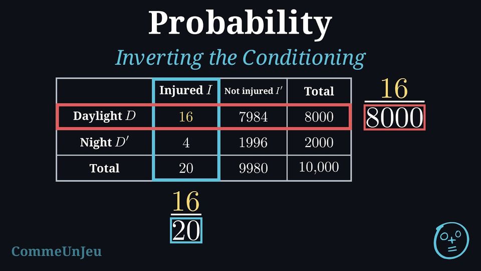
\(\PCond{A}{B}\) and \(\PCond{B}{A}\) are not equal in general: they share the numerator \(\Card{A \cap B}\), but one divides by \(\Card{B}\) and the other by \(\Card{A}\). Everyday sentences often slide from one to the other. Take the bicycle rides made in a town during a year, and let \(D\) be “the ride is made in daylight” and \(I\) be “the cyclist is injured during the ride”. “Most of the injured cyclists were riding in daylight” is about \(\PCond{D}{I}\), which would be large even if daylight were no more dangerous than night, simply because most rides are made in daylight; by itself it says nothing about \(\PCond{I}{D}\), the risk of a daytime ride. A two-way table of counts keeps the two apart: the known event chooses the row or the column, hence the denominator.
Example
In a population, \(1\pourcent\) of the people have a certain illness. A screening test is positive for \(99\pourcent\) of the ill people (its sensitivity) and negative for \(95\pourcent\) of the healthy people (its specificity). A person is chosen at random; let \(M\) be “the person is ill” and \(T\) be “the test is positive”. - Fill in a two-way table of counts for a population of \(10\,000\) people.
- Compute \(\PCond{T}{M}\) and \(\PCond{M}{T}\), and compare them.
- Out of \(10\,000\) people, \(1\pourcent\) are ill: \(100\) ill and \(9\,900\) healthy. The test is positive for \(99\pourcent\) of the \(100\) ill people, that is \(99\) true positives, and negative for the other \(1\), a false negative. It is negative for \(95\pourcent\) of the \(9\,900\) healthy people, that is \(9\,405\), and positive for the other \(495\).
Test positive \(T\) Test negative \(T'\) Total Ill \(M\) \(99\) \(1\) \(100\) Healthy \(M'\) \(495\) \(9\,405\) \(9\,900\) Total \(594\) \(9\,406\) \(10\,000\) - The known event chooses the denominator: $$\begin{aligned} \PCond{T}{M} &= \frac{\Card{M \cap T}}{\Card{M}} = \frac{99}{100}, \\ \PCond{M}{T} &= \frac{\Card{M \cap T}}{\Card{T}} = \frac{99}{594} = \frac{1}{6}. \end{aligned}$$ Among the \(100\) ill people, \(99\) test positive; but among the \(594\) people who test positive, only \(99\) are ill, one out of six, because the \(495\) false positives outnumber the \(99\) true positives: the illness is rare, so the healthy people, even with a small error rate, supply most of the positive results.
Skills to practice
- Inverting the Conditioning: False Positives
II.3
Probability Trees
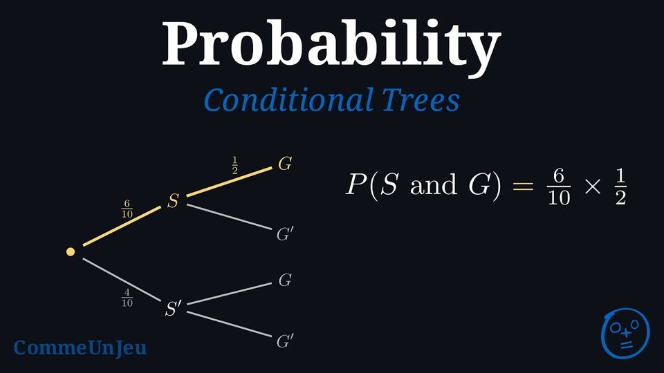
From the Table to the Tree
The two-way table of the \(100\) students can be read in two stages: first the gender, then, within the chosen gender, whether the pupil loves maths. Drawn as branches, these two stages make a tree: a first level with \(P(\text{Girl}) = \frac{51}{100}\) and \(P(\text{Boy}) = \frac{49}{100}\), then, along the “Girl” branch, \(\PCond{\text{Loves Maths}}{\text{Girl}} = \frac{35}{51}\) and \(\PCond{\text{Does Not Love Maths}}{\text{Girl}} = \frac{16}{51}\). The second-level branches carry conditional probabilities: that is what makes it a conditional probability tree, and what the Definition “Conditional Probability Tree Diagram” sets down.
Definition — Conditional Probability Tree Diagram
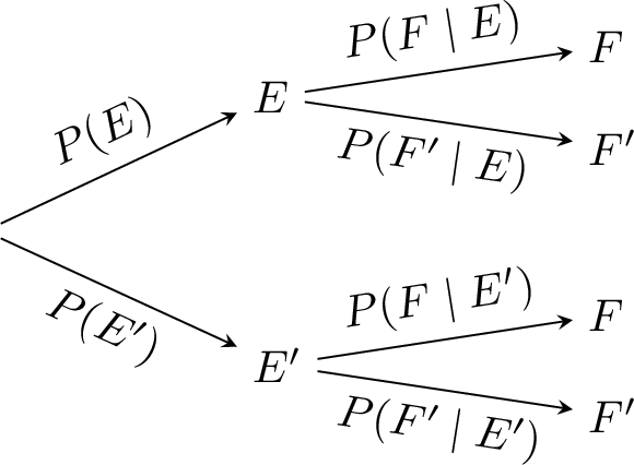
A conditional probability tree visually organizes probabilities for a sequence of events: - Each branch from a node shows either an unconditional probability (e.g. \(P(E)\)) or a conditional probability (e.g. \(\PCond{F}{E}\)).
- Events are labelled at the end of each branch.
- The probabilities on the branches leaving one node add up to \(1\) (sum rule): for instance \(\PCond{F'}{E} = 1 - \PCond{F}{E}\).
- The probability of the intersection of the events met along a path is the product of the probabilities along that path (product rule).
Example
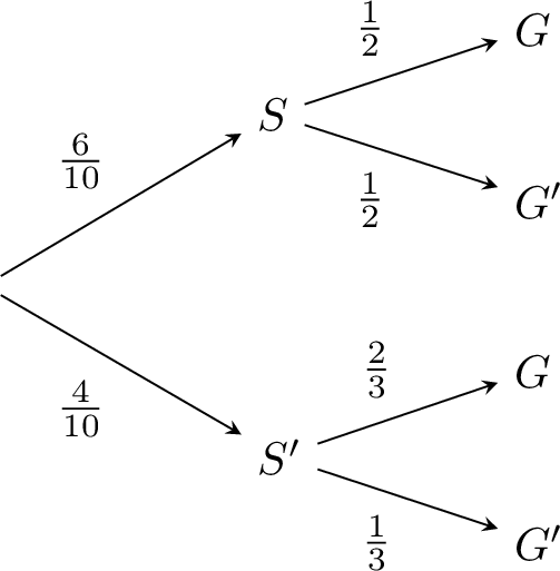
The probability Sam coaches a game is \(\frac{6}{10}\), and the probability Alex coaches is \(\frac{4}{10}\). If Sam coaches, the probability that a randomly selected player is a goalkeeper is \(\frac{1}{2}\); if Alex coaches, it is \(\frac{2}{3}\).Draw the tree diagram.
- Define the events:
- \(S\): Sam coaches.
- \(G\): Player is goalkeeper.
- Define the probabilities:
- \(P(S) = \frac{6}{10}\) and \(P(S') =1 - P(S)= \frac{4}{10}\).
- \(\PCond{G}{S} = \frac{1}{2}\) and \(\PCond{G'}{S} = 1 - \PCond{G}{S} = \frac{1}{2}\).
- \(\PCond{G}{S'} = \frac{2}{3}\) and \(\PCond{G'}{S'} = 1-\PCond{G}{S'}= \frac{1}{3}\).
- Tree diagram:
Skills to practice
- Identifying Conditional Probability Tree Diagrams
II.4
Joint Probability
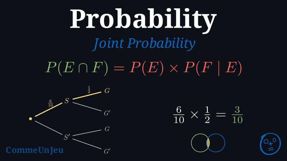
Sometimes we know \(P(E)\) and \(\PCond{F}{E}\) and need the chance both \(E\) and \(F\) happen together—like finding the probability that a student is a girl who loves maths. This probability is called the joint probability \(P(E \cap F)\).
Proposition — Joint Probability Formula
For \(P(E) > 0\) and \(P(F) > 0\) respectively: $$P(E \cap F) = P(E) \times \PCond{F}{E}, \quad P(E \cap F) = P(F) \times \PCond{E}{F}.$$
By definition, for \(P(E) > 0\), \(\PCond{F}{E} = \dfrac{P(E \cap F)}{P(E)}\); multiplying both sides by \(P(E)\) gives \(P(E \cap F) = P(E) \times \PCond{F}{E}\). The second identity is the same statement with the roles of \(E\) and \(F\) exchanged, for \(P(F) > 0\).
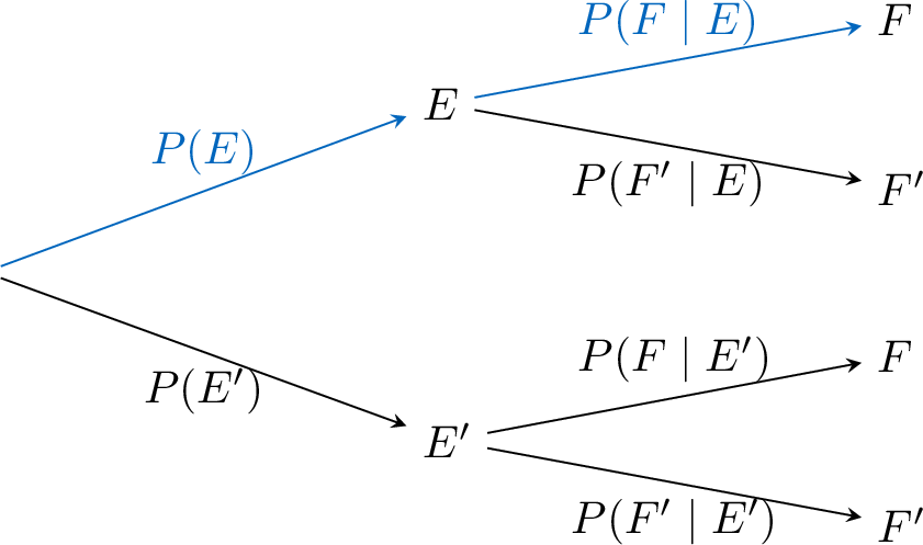
Method — Finding \(P(E \cap F)\) in a Tree
- Identify the path where \(E\) and \(F\) both occur.
- Multiply the probabilities along that path.
Example
For this probability tree, - Path: \(S\) to \(G\) (highlighted):
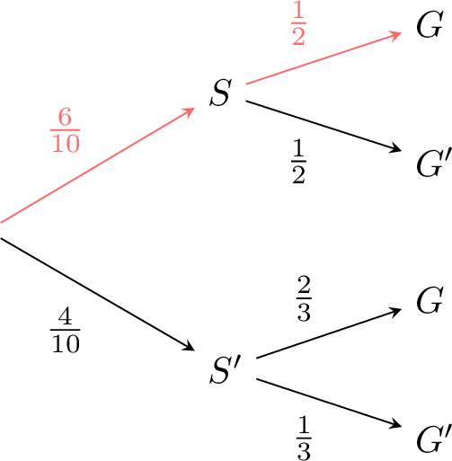
- Calculate: $$\begin{aligned} P(S \cap G) &= P(S) \times \PCond{G}{S}\\ &= \frac{6}{10} \times \frac{1}{2}\\ &= \frac{3}{10}. \end{aligned}$$
Skills to practice
- Calculating Joint Probabilities with Trees
II.5
Law of Total Probability
Two Paths to the Same Event
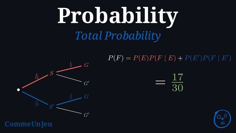
In a two-stage tree, the event \(F\) appears at the end of two paths: through \(E\), and through \(E'\). Each path has its probability, the product along its branches. The two paths cannot both happen, since \(E\) and \(E'\) are mutually exclusive, and together they cover every way for \(F\) to happen, since \(E\) and \(E'\) are complementary. So the probability of \(F\) is the sum of the two path probabilities. Written with conditional probabilities, this is the law of total probability.
Theorem — Law of Total Probability
For events \(E\) and \(F\) with \(0 < P(E) < 1\): $$P(F) = P(E) \PCond{F}{E} + P(E') \PCond{F}{E'}.$$ This applies when \(E\) and its complement \(E'\) form a partition of the sample space. More generally, if \((E_1,\dots,E_n)\) is a partition of the sample space into events of non-zero probability, then $$P(F) = \sum_{i=1}^n P(E_i)\PCond{F}{E_i}.$$
Let \(\{E_1, E_2, \dots, E_n\}\) be a partition of the sample space and let \(F\) be any event. The proposition Partition Induced on an Event cuts \(F\) into the pieces \(F \cap E_1, \dots, F \cap E_n\): they are pairwise mutually exclusive, and their union is \(F\). That is exactly what the additivity of probabilities for mutually exclusive events needs. $$\begin{aligned}[t] F &= (F \cap E_1) \cup \dots \cup (F \cap E_n) && \text{(the partition cuts \(F\))}\\
P(F) &= P(F \cap E_1) + \dots + P(F \cap E_n) && \text{(additivity --- the pieces are pairwise exclusive)}\\
&= P(E_1)\PCond{F}{E_1} + \dots + P(E_n)\PCond{F}{E_n} && \text{(joint probability formula, on each piece)}\\
&= \sum_{i=1}^{n} P(E_i)\PCond{F}{E_i} \end{aligned}$$ The two-piece statement is this same result applied to the partition \(\{E, E'\}\): $$P(F) = P(E)\PCond{F}{E} + P(E')\PCond{F}{E'}.$$ Each piece is read on the tree as one path down to \(F\), which is why summing the paths gives \(P(F)\).
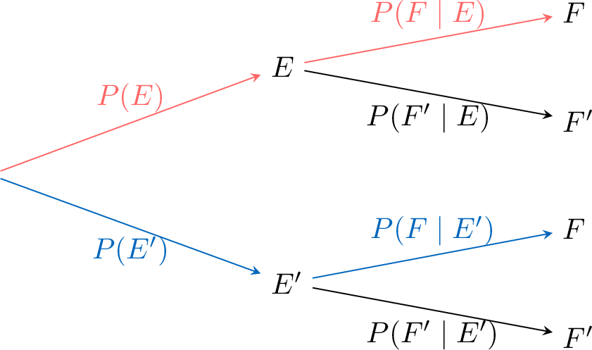
Method — Finding \(P(F)\) in a Tree
- Identify all paths to \(F\).
- Multiply probabilities along each path and sum them.
Example
For this probability tree, - Paths to \(G\):
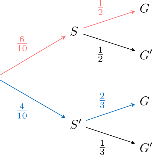
- Calculate: $$\begin{aligned} P(G) &= \textcolor{colordef}{\frac{6}{10} \times \frac{1}{2}} + \textcolor{colorprop}{\frac{4}{10} \times \frac{2}{3}} \\ &= \textcolor{colordef}{\frac{3}{10}} + \textcolor{colorprop}{\frac{8}{30}} \\ &= \textcolor{colordef}{\frac{9}{30}} + \textcolor{colorprop}{\frac{8}{30}} \\ &= \frac{17}{30}. \end{aligned}$$
Example
A disease affects \(2\pourcent\) of a population. A screening test is positive for \(95\pourcent\) of the people who are ill, and also for \(10\pourcent\) of the people who are healthy. A person is chosen at random and tested; let \(E\) be “the person is ill” and \(F\) be “the test is positive”. Compare \(\PCond{F}{E}\) and \(\PCond{E}{F}\).
\(\PCond{F}{E} = 0.95\) is given: the probability of a positive test knowing that the person is ill. The other one, \(\PCond{E}{F}\), is the probability of being ill knowing that the test is positive; it is not given, and it is what a tested person wants to know. $$\begin{aligned}[t] P(E') &= 1 - P(E) = 1 - 0.02 = 0.98 && \scriptscriptstyle\text{(complement rule)} \\
P(E \cap F) &= P(E) \times \PCond{F}{E} && \scriptscriptstyle\text{(product rule)} \\
&= 0.02 \times 0.95 = 0.019 \\
P(F) &= P(E)\,\PCond{F}{E} + P(E')\,\PCond{F}{E'} && \scriptscriptstyle\text{(total probability)} \\
&= 0.019 + 0.98 \times 0.10 = 0.117 \\
\PCond{E}{F} &= \frac{P(E \cap F)}{P(F)} && \scriptscriptstyle\text{(definition)} \\
&= \frac{0.019}{0.117} \approx 0.16 \end{aligned}$$ So \(\PCond{F}{E} = 0.95\) but \(\PCond{E}{F} \approx 0.16\): among the positive tests, only about one in six comes from an ill person, because the healthy are far more numerous and \(10\pourcent\) of them also test positive. The two conditional probabilities answer two different questions. Reversing a conditioning this way has a name and a formula: Bayes' theorem.
Three Paths to the Same Event
The first step of an experiment may have three outcomes rather than two: a part is made by one of three machines \(M_1\), \(M_2\), \(M_3\), each of which makes some of the parts. Each part comes from exactly one machine: two of these events cannot happen together, and one of them always happens — the three events form a partition of the sample space. The tree then has three branches at its root, and an event \(F\) is reached by three paths, one through each \(M_i\). The three paths cannot happen together, and together they cover every way for \(F\) to happen; each path has for probability the product along its branches. So the probability of \(F\) is the sum of the three path probabilities: $$\textcolor{colorprop}{P(F) = P(M_1)\PCond{F}{M_1} + P(M_2)\PCond{F}{M_2} + P(M_3)\PCond{F}{M_3}}.$$ The reasoning is the one of the two-path case: it does not depend on the number of branches.
Example
A factory makes bolts on three machines: \(M_1\) makes \(50\pourcent\) of them, \(M_2\) makes \(30\pourcent\) and \(M_3\) makes \(20\pourcent\). The proportions of defective bolts are \(2\pourcent\) for \(M_1\), \(3\pourcent\) for \(M_2\) and \(5\pourcent\) for \(M_3\). A bolt is chosen at random; \(D\) is the event “the bolt is defective”. - Draw the weighted tree.
- Compute \(P(D)\).
- The bolt chosen is defective. What is the probability that it was made by \(M_3\)? Round to \(10^{-3}\).
-
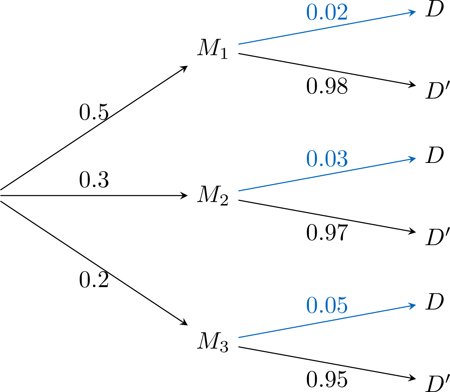
- \(M_1\), \(M_2\), \(M_3\) form a partition (each bolt comes from exactly one machine). Three paths lead to \(D\):
\(\begin{aligned}[t]P(D) &= P(M_1)\PCond{D}{M_1} + P(M_2)\PCond{D}{M_2} + P(M_3)\PCond{D}{M_3} &&\text{(total probability)}\\ &= 0.5 \times 0.02 + 0.3 \times 0.03 + 0.2 \times 0.05\\ &= 0.01 + 0.009 + 0.01\\ &= 0.029\end{aligned}\) - \(\begin{aligned}[t]\PCond{M_3}{D} &= \dfrac{P(M_3 \cap D)}{P(D)} &&\text{(definition)}\\ &= \dfrac{0.2 \times 0.05}{0.029}\\ &= \dfrac{0.01}{0.029}\\ &\approx 0.345\end{aligned}\)
\(M_3\) makes only \(20\pourcent\) of the bolts, but about \(34.5\pourcent\) of the defective ones.
Skills to practice
- Calculating Probabilities with Trees
- Calculating Probabilities in Context
- Using a Partition into Three Events
- Justifying and Using the Law of Total Probability
III
Going further
Skills to practice
- Solving Two-Way Table Problems
- Solving Conditional Probability Problems
- Quiz
Jump to section