International Baccalaureate · DP 2: Applications and Interpretation HL

Chi-squared Tests

⌚ ~82 min ▢ 8 blocks ✓ 33 exercises ➣ Prerequisites : Hypothesis Testing, Discrete Random Variables, The Normal Distribution

I The Test for Independence

I.1 The Chi-squared Test for Independence

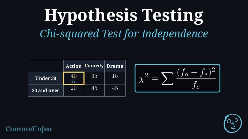
Every test so far has compared numerical measurements, such as means. The chi-squared test extends hypothesis testing to categorical data. In this sense it is the categorical analogue of correlation: a correlation coefficient measures the association between two numerical variables, while the chi-squared test of independence asks whether two categorical variables are associated.

Report an error

Definition — Two-Way Table of Counts

Two qualitative variables are observed on the same population of $N$ individuals. The two-way table of counts has one row for each category of the first variable and one column for each category of the second; the cell at row $A$ and column $B$ holds the count of the individuals that have both categories $A$ and $B$, written $n(A \cap B)$.

The last column holds the row totals: $n(A)$ is the number of individuals of category $A$.
The last row holds the column totals: $n(B)$ is the number of individuals of category $B$.
The bottom-right cell holds the grand total $N$, which is the sum of the row totals and the sum of the column totals.

The Chi-squared ($\chi^2$) test for independence determines if there is a significant association between two categorical variables. It compares the observed frequencies in a contingency table to the frequencies we would expect if the variables were completely independent.

Report an error

Definition — Observed and Expected Frequencies

Observed Frequencies ($f_o$): The actual data collected and recorded in a contingency table.
Expected Frequencies ($f_e$): The theoretical counts calculated assuming the variables are independent.

The formula for the expected frequency of a cell is:$$ f_e = \frac{\text{Row Total} \times \text{Column Total}}{\text{Grand Total}} $$

Definition — Chi-squared Statistic

The test statistic $\chi^2_{calc}$ measures the total deviation between observed and expected values:$$ \chi^2_{calc} = \sum \frac{(f_o - f_e)^2}{f_e} $$ The degrees of freedom ($df$) for a table with $r$ rows and $c$ columns is:$$ \mathrm{d}f = (r - 1)(c - 1) $$

Method — Steps for a Chi-squared Test

Step 1: Write the Hypotheses
- $H_0$: The variables are independent.
- $H_1$: The variables are not independent (associated).
Step 2: Enter data into GDC
- Enter the observed contingency table into a Matrix (e.g., Matrix A).
- Select $\chi^2$-Test (usually under Stat $\to$ Tests).
Step 3: Analyze Results
The calculator provides $\chi^2_{calc}$, the p-value, and the degrees of freedom ($df$).
Note: As a rule of thumb, all expected frequencies should be at least 5 for the test to be reliable.
Step 4: Conclusion
Compare the p-value to the significance level $\alpha$.
- If $p\text{-value} < \alpha$: Reject $H_0$ (Variables are dependent/associated).
- If $p\text{-value} \geq \alpha$: Fail to reject $H_0$ (No evidence of association).

Example

A survey asked 200 people about their preferred type of movie and their age group. The results are shown below:

	Action	Comedy	Drama
Under 30	40	35	15
30 and over	20	45	45

Test at the 5$\pourcent$ significance level whether age group and movie preference are independent.

Answer

Step 1: Hypotheses
$H_0$: Age group and movie preference are independent.
$H_1$: Age group and movie preference are not independent (they are associated).
Step 2: Calculator
Enter the $2 \times 3$ matrix into the calculator and run the $\chi^2$-Test.
- $\chi^2_{calc} \approx 21.1$
- $\mathrm{d}f = (2-1)(3-1) = 2$
- $p\text{-value} \approx 0.000026$ (about $2.6 \times 10^{-5}$)
Step 3: Conclusion
$0.000026 < 0.05$. Since $p < \alpha$, we reject $H_0$.
There is strong evidence to suggest that movie preference depends on age group.

Method — Deciding with a $\chi^2$ Critical Value

The statistic $\chi^2_{calc}$ is never negative, and it grows as the observed frequencies move away from the expected ones: only large values count against $H_0$, so a $\chi^2$ test is always upper-tailed. Its critical value $\chi^2_{crit}$ is the number such that $P(\chi^2 \geq \chi^2_{crit}) = \alpha$ for the $\chi^2$ distribution with the degrees of freedom $\nu$ of the test; it is read in a table or given in the question.

Expected frequencies: compute them, and check that each one is greater than $5$.
Statistic: $\chi^2_{calc} = \sum \dfrac{(f_o - f_e)^2}{f_e}$, by hand for a small table or with the calculator, and the degrees of freedom $\nu$.
Decision: reject $H_0$ if $\chi^2_{calc} \geq \chi^2_{crit}$; otherwise do not reject it. It is the same decision as rejecting when $p\text{-value} \leq \alpha$.

$\nu$	$1$	$2$	$3$	$4$	$5$	$6$	$9$
$\alpha = 0.10$	$2.706$	$4.605$	$6.251$	$7.779$	$9.236$	$10.645$	$14.684$
$\alpha = 0.05$	$3.841$	$5.991$	$7.815$	$9.488$	$11.070$	$12.592$	$16.919$
$\alpha = 0.01$	$6.635$	$9.210$	$11.345$	$13.277$	$15.086$	$16.812$	$21.666$

Example

A café asks $150$ customers whether they prefer coffee or tea, and notes their age group.

	Coffee	Tea
Under $40$	$45$	$30$
$40$ and over	$25$	$50$

By computing the expected frequencies and the statistic by hand, test at the $5\pourcent$ significance level whether the preferred drink is independent of the age group, using the critical value.

Answer

$H_0$: the preferred drink is independent of the age group; $H_1$: it is not.
The row totals are $75$ and $75$, the column totals $70$ (coffee) and $80$ (tea), the grand total $150$. For the cell “under $40$, coffee”: $$f_e = \frac{\text{row total} \times \text{column total}}{\text{grand total}} = \frac{75 \times 70}{150} = 35,$$ and likewise $40$ for “under $40$, tea”, $35$ and $40$ for the second row: all greater than $5$.
Every cell is $10$ away from its expected frequency: $$\begin{aligned}[t] \chi^2_{calc} &= \sum \frac{(f_o - f_e)^2}{f_e} && \text{(statistic)} \\ &= \frac{10^2}{35} + \frac{10^2}{40} + \frac{10^2}{35} + \frac{10^2}{40} \\ &\approx 2.857 + 2.5 + 2.857 + 2.5 \approx 10.71, \end{aligned}$$ with $\nu = (2 - 1)(2 - 1) = 1$.
At $\alpha = 0.05$ and $\nu = 1$, $\chi^2_{crit} = 3.841$. Since $10.71 > 3.841$, reject $H_0$ (the calculator gives $p\text{-value} \approx 0.00106$, the same decision).
At the $5\pourcent$ level, the preferred drink depends on the age group: the younger customers lean towards coffee, the older towards tea.

Skills to practice

Deciding with a Critical Value
Computing Expected Frequencies and Degrees of Freedom
Conducting Chi-squared Tests for Independence

II Goodness of Fit

II.1 The Chi-squared Goodness of Fit Test

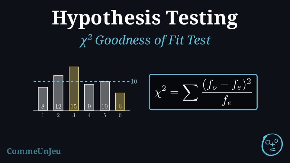
The Goodness of Fit (GOF) test is used to determine whether a variable is likely to come from a specified distribution (such as Uniform, Binomial, Normal, or a specific ratio). It compares the observed data with what we would expect theoretically.

Report an error

Definition — Goodness of Fit Statistic

The test uses the same $\chi^2$ statistic formula:$$ \chi^2_{calc} = \sum \frac{(f_o - f_e)^2}{f_e} $$ However, the degrees of freedom ($df$) calculation depends on the distribution:$$ \mathrm{d}f = k - 1 - m $$ Where:

$k$ is the number of categories (bins).
$m$ is the number of population parameters estimated from the sample data (e.g., if you calculate mean and standard deviation from the sample to fit a Normal distribution, $m=2$).

Method — Steps for a GOF Test

Step 1: Hypotheses
- $H_0$: The data follow the specified distribution.
- $H_1$: The data do not follow the specified distribution.
Step 2: Expected Frequencies
Calculate the expected frequency for each category: $$ f_e = n \times P(\text{category}) $$ (As for the independence test, all expected frequencies should be at least 5 for the $\chi^2$ approximation to be reliable.) Note: Usually done in List 2 of the GDC.
Step 3: Calculator
- Enter observed values in List 1 ($f_o$).
- Enter expected values in List 2 ($f_e$).
- Select $\chi^2$ GOF Test.
- Enter the correct $df$.
Step 4: Conclusion
Compare p-value to $\alpha$ and interpret in context.

Example

A die is rolled 60 times. The results are:

Outcome	1	2	3	4	5	6
Frequency	8	12	15	9	10	6

Test at the 5$\pourcent$ level if the die is fair (Uniform distribution).

Answer

Hypotheses:
$H_0$: The die is fair (Uniform distribution).
$H_1$: The die is not fair.
Expected Frequencies:
Total $n=60$. If fair, $P(X=k) = 1/6$. $$ f_e = 60 \times \frac{1}{6} = 10 \quad \text{for all outcomes} $$
Calculator / Working:
$L_1: \{8, 12, 15, 9, 10, 6\}$
$L_2: \{10, 10, 10, 10, 10, 10\}$ $$ \chi^2_{calc} = \sum \frac{(f_o - f_e)^2}{f_e} = \frac{(8-10)^2}{10} + \frac{(12-10)^2}{10} + \cdots + \frac{(6-10)^2}{10} = 5.0 $$ Degrees of freedom: $\mathrm{d}f = k - 1 = 6 - 1 = 5$ (no parameters estimated).
$p\text{-value} \approx 0.416$.
Conclusion:
$0.416 > 0.05$. We fail to reject $H_0$: there is insufficient evidence at the 5\,$\pourcent$ level to conclude the die is unfair.

Skills to practice

Finding Expected Frequencies for a Goodness of Fit
Conducting Chi-squared Goodness of Fit Tests

II.2 Goodness of Fit with Estimated Parameters

When the Model Is Not Fully Given

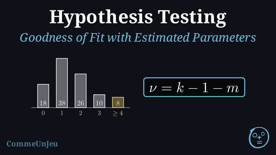
In the goodness-of-fit tests met so far, the model was given in full: a fair die, a ratio $9:3:3:1$, a binomial distribution with known $n$ and $p$. Often only the family of the model is claimed — “the counts follow a Poisson distribution”, “the heights are normally distributed” — and its parameters are estimated from the same data: $\lambda$ by the sample mean $\bar{x}$, $p$ by $\dfrac{\bar{x}}{n}$ for $\mathcal{B}(n, p)$, $\mu$ and $\sigma$ by $\bar{x}$ and $s_{n-1}$. Parameters fitted to the data make the model follow these very data more closely than a model fixed in advance would, so $\chi^2_{calc}$ tends to be smaller: to compensate, each estimated parameter costs one degree of freedom, $\nu = k - 1 - m$ (the usual rule, an approximation that works well in practice). When the data are numerical, the test also needs categories: values or intervals chosen so that every expected frequency is greater than $5$.

Report an error

Method — Testing the Fit of a Model with Estimated Parameters

Hypotheses: $H_0$: the data follow a distribution of the claimed family (Poisson, binomial, normal); $H_1$: they do not.
Estimates: $\lambda = \bar{x}$ for a Poisson model; $p = \dfrac{\bar{x}}{n}$ for $\mathcal{B}(n, p)$; $\mu = \bar{x}$ and $\sigma = s_{n-1}$ for a normal model.
Categories and probabilities: for a discrete model, one category per value and a last open category “$\geq k$”, so that the probabilities add up to $1$; for a normal model, class intervals whose first and last classes are open (below the first bound, above the last).
Expected frequencies: $f_e = N \times P(\text{category})$, with $N$ the number of observations; combine adjacent categories, and their observed frequencies with them, until every expected frequency is greater than $5$.
Degrees of freedom: $\nu = k - 1 - m$, with $k$ the number of categories after combining and $m$ the number of estimated parameters; $\nu$ must be at least $1$, otherwise there are too few categories for the number of estimated parameters and the test cannot be carried out.
Test: run the $\chi^2$ goodness-of-fit test of the calculator, entering $\nu$ by hand — the calculator does not know how many parameters were estimated — or compare $\chi^2_{calc}$ with the critical value for $\nu$.

Example

Over $100$ one-minute intervals, the number of customers arriving at a ticket counter is recorded; no interval had more than $5$ customers.

Customers	$0$	$1$	$2$	$3$	$4$	$5$
Intervals	$18$	$38$	$26$	$10$	$5$	$3$

Test at the $5\pourcent$ significance level whether a Poisson distribution fits these data.

Answer

$H_0$: the number of customers per minute follows a Poisson distribution; $H_1$: it does not.
The parameter is estimated by the mean number of customers per minute: $$\lambda = \bar{x} = \frac{0 \times 18 + 1 \times 38 + 2 \times 26 + 3 \times 10 + 4 \times 5 + 5 \times 3}{100} = \frac{155}{100} = 1.55.$$
With $X \sim \mathcal{P}(1.55)$ and $N = 100$, the expected frequencies are $100\,P(X = k)$, the last category “$\geq 4$” taking $1 - P(X \leq 3)$:

Customers $0$ $1$ $2$ $3$ $\geq 4$

$f_o$ $18$ $38$ $26$ $10$ $8$

$f_e$ $21.22$ $32.90$ $25.50$ $13.17$ $7.21$

Kept apart, the value $4$ would expect $5.10$ intervals and “$\geq 5$” only $2.10$: the two are combined into “$\geq 4$”, whose observed frequency is $5 + 3 = 8$.
$k = 5$ categories and $m = 1$ estimated parameter: $\nu = 5 - 1 - 1 = 3$.
The $\chi^2$ goodness-of-fit test with $\nu = 3$ gives $\chi^2_{calc} \approx 2.14$ and $p\text{-value} \approx 0.543$. Since $0.543 > 0.05$ (equivalently $2.14 < 7.815$), $H_0$ is not rejected: at the $5\pourcent$ level, a Poisson distribution with mean $1.55$ is consistent with the arrivals.

Example

The heights, in cm, of $200$ plants of a nursery are grouped in classes. From the raw data, $\bar{x} = 27.4$ and $s_{n-1} = 5.1$.

Height	$< 20$	$20$–$24$	$24$–$28$	$28$–$32$	$32$–$36$	$\geq 36$
Plants	$10$	$38$	$74$	$42$	$20$	$16$

Test at the $5\pourcent$ significance level whether the heights are normally distributed.

Answer

$H_0$: the heights follow a normal distribution; $H_1$: they do not.
The parameters are estimated from the data: $\mu = 27.4$ and $\sigma = 5.1$, so the model is $X \sim \mathcal{N}(27.4, 5.1^2)$.

Each expected frequency is $200$ times the probability of its class, the first and last classes being open. For the first: $$\begin{aligned}[t] f_e &= 200\,P(X < 20) = 200\,P\left(Z < \frac{20 - 27.4}{5.1}\right) \\ &\approx 200 \times 0.0734 \approx 14.68, \end{aligned}$$ and in the same way:

Height	$< 20$	$20$–$24$	$24$–$28$	$28$–$32$	$32$–$36$	$\geq 36$
$f_o$	$10$	$38$	$74$	$42$	$20$	$16$
$f_e$	$14.68$	$35.82$	$58.87$	$53.93$	$27.53$	$9.17$

All the expected frequencies are greater than $5$: no class is combined.

$k = 6$ classes and $m = 2$ estimated parameters: $\nu = 6 - 1 - 2 = 3$.
The $\chi^2$ goodness-of-fit test with $\nu = 3$ gives $\chi^2_{calc} \approx 15.29$ and $p\text{-value} \approx 0.00158$. Since $0.00158 \leq 0.05$ (equivalently $15.29 > 7.815$), $H_0$ is rejected: at the $5\pourcent$ level, the heights are not normally distributed — there are too many plants in the middle class and in the tallest class for a symmetric bell curve.

Skills to practice

Counting Degrees of Freedom
Testing the Fit of a Model

III Going further

Skills to practice

Problems: Choosing and Carrying Out Tests
Quiz

\(\nu\)	\(1\)	\(2\)	\(3\)	\(4\)	\(5\)	\(6\)	\(9\)
\(\alpha = 0.10\)	\(2.706\)	\(4.605\)	\(6.251\)	\(7.779\)	\(9.236\)	\(10.645\)	\(14.684\)
\(\alpha = 0.05\)	\(3.841\)	\(5.991\)	\(7.815\)	\(9.488\)	\(11.070\)	\(12.592\)	\(16.919\)
\(\alpha = 0.01\)	\(6.635\)	\(9.210\)	\(11.345\)	\(13.277\)	\(15.086\)	\(16.812\)	\(21.666\)

	Coffee	Tea
Under \(40\)	\(45\)	\(30\)
\(40\) and over	\(25\)	\(50\)

Customers	\(0\)	\(1\)	\(2\)	\(3\)	\(4\)	\(5\)
Intervals	\(18\)	\(38\)	\(26\)	\(10\)	\(5\)	\(3\)

Customers	\(0\)	\(1\)	\(2\)	\(3\)	\(\geq 4\)
\(f_o\)	\(18\)	\(38\)	\(26\)	\(10\)	\(8\)
\(f_e\)	\(21.22\)	\(32.90\)	\(25.50\)	\(13.17\)	\(7.21\)

Height	\(< 20\)	\(20\)–\(24\)	\(24\)–\(28\)	\(28\)–\(32\)	\(32\)–\(36\)	\(\geq 36\)
Plants	\(10\)	\(38\)	\(74\)	\(42\)	\(20\)	\(16\)