International Baccalaureate · DP 1: Applications and Interpretation HL

Probability

⌚ ~122 min ▢ 13 blocks ✓ 55 exercises PDFFull lesson PDFExercise sheet PDFSolutions ➣ Prerequisites : Sets and Venn Diagrams

I The World of Events

I.1 Experiments, Sample Spaces and Events

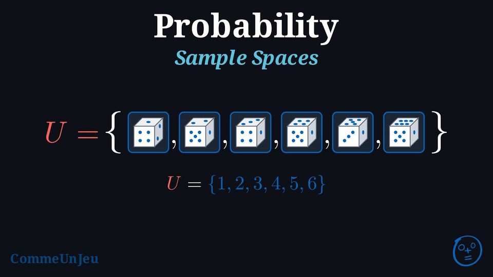
Some actions have a result we cannot predict — flipping a coin, rolling a die, or playing a game. We call such an action a random experiment: it can be repeated under the same conditions, all its possible results are known in advance, but nobody can tell with certainty which one will happen. Probability is a mathematical way to measure how likely an event of the experiment is, such as “rolling a 6” when a die is rolled.

Report an error

Definition — Sample Space

The sample space, denoted $U$, is the set of all possible outcomes of a random experiment. A single outcome is denoted $x$. If the experiment has $n$ outcomes, we write $$U = \{x_1, x_2, \dots, x_n\}.$$

Definition — Event

An event (often denoted by a capital letter like $E$) is a subset of the sample space.

Skills to practice

Writing an Event as a Set of Outcomes

I.2 Sample Space Diagrams

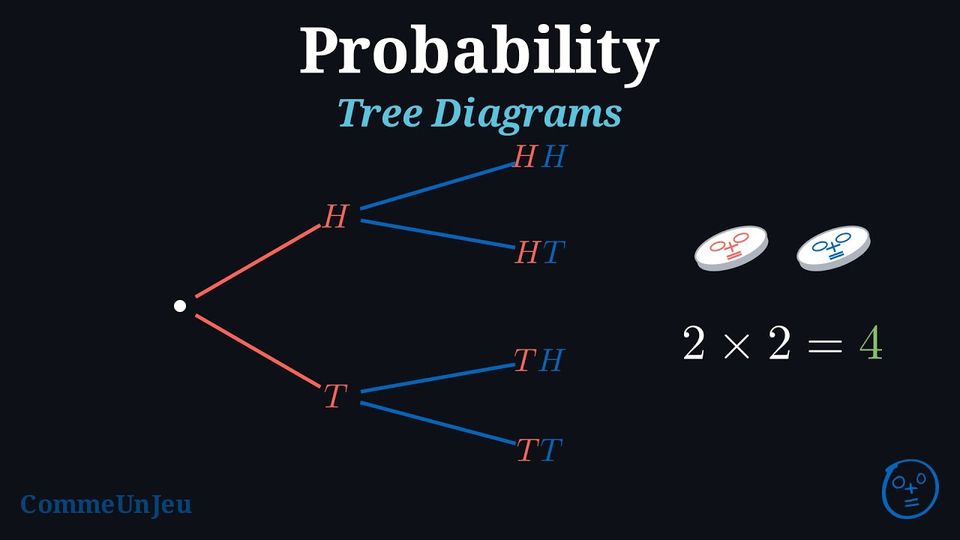
A multi-step experiment is a random experiment made up of a sequence of two or more simple steps. For example, flipping two coins is a multi-step experiment composed of two actions: flipping the first coin and then flipping the second.
In many multi-step experiments, we can find the total number of possible outcomes by multiplying the number of outcomes at each step. To display all the combined outcomes, we can use tools like lists, tables, or tree diagrams.

Report an error

Method — Representing Sample Spaces for Multi-Step Experiments

When an experiment has more than one step, the sample space can be represented in several ways:

by listing all possible ordered outcomes;
using a table (best for two-step experiments);
using a tree diagram (useful for any number of steps).

Example

For the experiment of tossing two coins, represent the sample space by:

listing all possible outcomes;
using a table;
using a tree diagram.

Answer

List:
Each outcome records the result of coin 1 first, then coin 2: $$\{\textcolor{colordef}{H}\textcolor{colorprop}{H}, \textcolor{colordef}{H}\textcolor{colorprop}{T}, \textcolor{colordef}{T}\textcolor{colorprop}{H}, \textcolor{colordef}{T}\textcolor{colorprop}{T}\}$$

Table:

$\begin{aligned} & \textcolor{colorprop}{\text{coin 2}} \\ \textcolor{colordef}{\text{coin 1}} \end{aligned} $	$\textcolor{colorprop}{H}$	$\textcolor{colorprop}{T}$
$\textcolor{colordef}{H}$	$\textcolor{colordef}{H}\textcolor{colorprop}{H}$	$\textcolor{colordef}{H}\textcolor{colorprop}{T}$
$\textcolor{colordef}{T}$	$\textcolor{colordef}{T}\textcolor{colorprop}{H}$	$\textcolor{colordef}{T}\textcolor{colorprop}{T}$

Tree diagram:

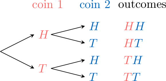
Skills to practice

Counting the Outcomes of an Event in a Table

I.3 Combining Events: Not, Or, And

Definition — Complementary Event

The complementary event of an event $E$, denoted $E'$ or $\overline{E}$, is the set of all outcomes in the sample space that are not in $E$.

Definition — $E$ or $F$

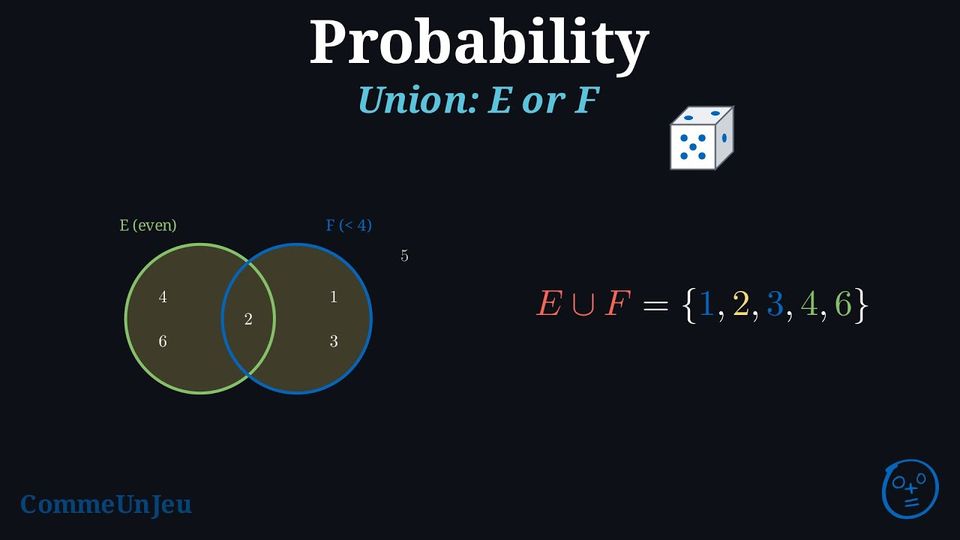
The union of two events $E$ and $F$, denoted $E \cup F$, is the event that occurs if $E$ occurs, or $F$ occurs, or both occur. We read this as “E or F”. It includes all outcomes that are in at least one of the events.

Definition — $E$ and $F$

The intersection of two events $E$ and $F$, denoted $E \cap F$, is the event that occurs if both $E$ and $F$ occur simultaneously. We read this as “E and F”. It includes all outcomes that are common to both events.

Definition — Mutually Exclusive

Two events $E$ and $F$ are mutually exclusive (or disjoint) if they have no outcomes in common. This means they cannot occur at the same time. Their intersection is the empty set ($\emptyset$): $$E \cap F = \emptyset.$$

Definition — Set Theory and Probability Vocabulary

Notation	Set Vocabulary	Probability Vocabulary	Venn Diagram
$U$	Universal set	Sample space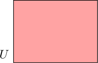
$x$	Element of $U$	Outcome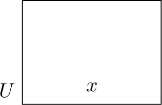
$\emptyset$	Empty set	Impossible event
$E$	Subset of $U$	Event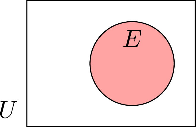
$x \in E$	$x$ is an element of $E$	$x$ is an outcome of $E$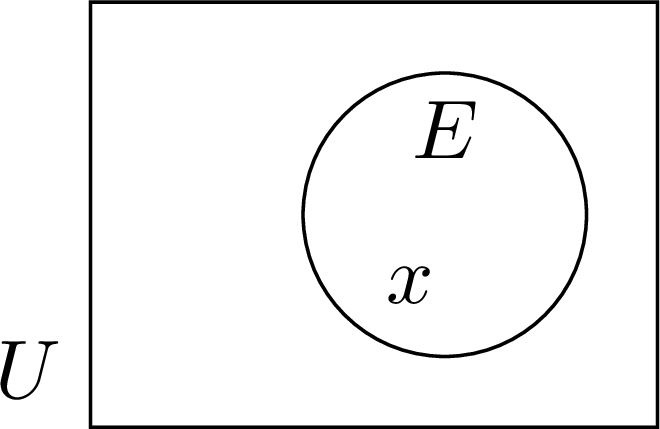
$E'$	Complement of $E$ in $U$	Complementary event of $E$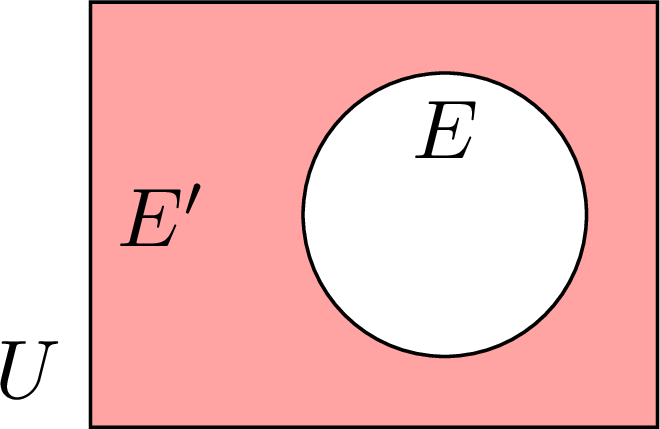
$E \cup F$	Union of $E$ and $F$	$E$ or $F$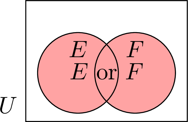
$E \cap F$	Intersection of $E$ and $F$	$E$ and $F$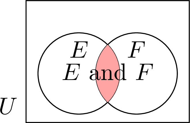
$E \cap F = \emptyset$	$E$ and $F$ are disjoint	$E$ and $F$ are mutually exclusive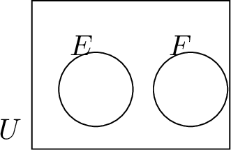

Skills to practice

Deciding whether Two Events Are Mutually Exclusive
Finding the Union of Two Events in a Venn Diagram
Finding Intersections and Complements in a Venn Diagram

I.4 Partitions of the Sample Space

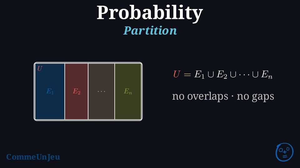
Definition — Partition of the Sample Space

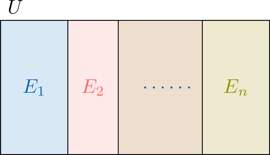
A partition of the sample space $U$ is a collection of events $E_1, E_2, \dots, E_n$ that are pairwise mutually exclusive and whose union is the sample space: every outcome of $U$ belongs to exactly one of them. In symbols:

they are pairwise mutually exclusive: $E_i \cap E_j = \emptyset$ whenever $i \neq j$;
they cover the whole sample space: $E_1 \cup E_2 \cup \dots \cup E_n = U$.

Proposition — Partition Induced on an Event

Let $\{E_1, E_2, \dots, E_n\}$ be a partition of the sample space $U$, and let $B$ be any event. Then the events $$\textcolor{colorprop}{B \cap E_1,\quad B \cap E_2,\quad \dots,\quad B \cap E_n}$$ are pairwise mutually exclusive, and their union is $B$: they form a partition of $B$.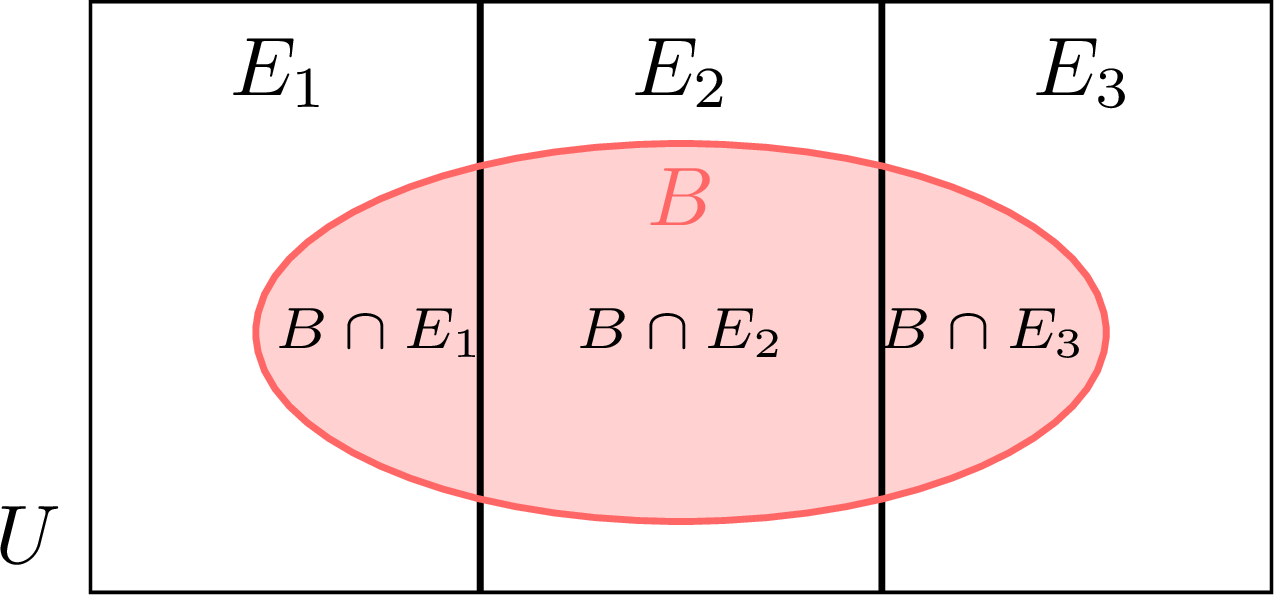

Proof

Everything rests on the equivalent formulation of the definition: every outcome of $U$ belongs to exactly one of $E_1, E_2, \dots, E_n$.

The pieces do not overlap. Take $i \neq j$. An outcome of $(B \cap E_i) \cap (B \cap E_j)$ would belong to $E_i$ and to $E_j$, whereas it belongs to at most one of the two. There is no such outcome: $$(B \cap E_i) \cap (B \cap E_j) = \emptyset.$$
The pieces give back $B$. An outcome of any $B \cap E_i$ is an outcome of $B$. Conversely, let $x$ be an outcome of $B$: it is an outcome of $U$, so it belongs to exactly one $E_i$; being in $B$ as well, it is in $B \cap E_i$. Every outcome of $B$ therefore lies in one of the pieces: $$(B \cap E_1) \cup (B \cap E_2) \cup \dots \cup (B \cap E_n) = B.$$

The pieces are pairwise mutually exclusive and cover $B$: they form a partition of $B$.

Skills to practice

Deciding whether Events Form a Partition

II Probability

II.1 Probability of an Event

An Event Is a Set and a Probability Is a Number

Rolling a fair die, the event “the result is even” is the set $A = \{2, 4, 6\}$; its probability is the number $P(A) = \frac{3}{6} = \frac{1}{2}$. Events combined with “or”, “and”, “not” measure nothing by themselves; a probability attaches a number to each event. The two objects must be kept apart, because two classic mistakes come from mixing them:

writing $P(A) = \{2, 4, 6\}$: a probability is never a set, $P(A)$ is the number $\frac{1}{2}$;
writing $A = \frac{1}{2}$ or saying “the event $A$ is one half”: an event is never a number, $A$ is a set of outcomes and $\frac{1}{2}$ is its probability.

The letter $P$ is a function: it takes an event $A \subseteq U$ and returns a number, its probability $P(A)$. Everything in this part says how that function behaves.

Report an error

Definition — Probability Axioms

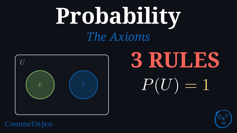
A function $P$ is a probability measure if it satisfies the following three axioms for any events $E$ and $F$ in a sample space $U$:

Axiom 1 (Non-negativity): The probability of any event is a non-negative number. $$P(E) \geq 0$$
Axiom 2 (Total Probability): The probability of the entire sample space is 1. $$P(U) = 1$$
Axiom 3 (Additivity for Mutually Exclusive Events): If two events $E$ and $F$ are mutually exclusive ($E \cap F = \emptyset$), then the probability of their union is the sum of their individual probabilities. $$P(E \cup F) = P(E) + P(F)$$

Everything else follows from these three statements — including the fact that a probability never exceeds $1$, proved below.

Definition — Equally Likely

When all outcomes are equally likely, the probability of an event $E$ is: $$\textcolor{colordef}{\begin{aligned} P(E) &= \frac{\text{number of outcomes in the event}}{\text{number of outcomes in the sample space}}\\ &=\dfrac{\Card{E}}{\Card{U}}\\ \end{aligned}}$$

Skills to practice

Writing the Event, then Computing Its Probability
Determining Events, then Their Probabilities

II.2 The Complement Rule and the Bounds of a Probability

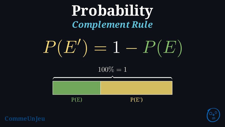
Proposition — Complement Rule

For any event $E$ and its complementary event $E'$, $$\textcolor{colorprop}{P(E') = 1 - P(E)}$$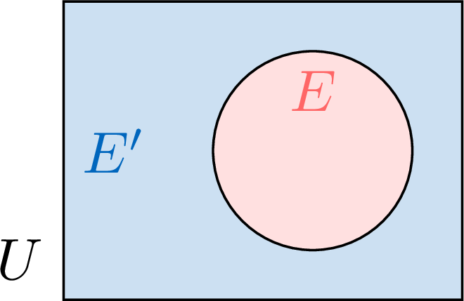

Proof

Algebraic Proof
By definition, an event $E$ and its complement $E'$ are mutually exclusive ($E \cap E' = \emptyset$) and their union is the entire sample space ($E \cup E' = U$).
Using Axiom 3: $P(E \cup E') = P(E) + P(E')$.
Using Axiom 2: $P(U) = 1$.
Since $E \cup E' = U$, we can equate their probabilities: $$ P(E) + P(E') = P(U) = 1. $$ Rearranging the formula gives the complement rule: $$P(E') = 1 - P(E).$$ In particular, the complement of the sample space $U$ is the impossible event, $U' = \emptyset$, so $$\begin{aligned}[t] P(\emptyset) &= P(U') && \text{($\emptyset$ is the complement of $U$)}\\ &= 1 - P(U) && \text{(complement rule)}\\ &= 1 - 1 && \text{(Axiom 2)}\\ &= 0. \end{aligned}$$ The impossible event has probability $0$.
Geometric Illustration
The total area of the sample space, $\textcolor{olive}{P(U)}$, , is the sum of the area of the event, $P(E)$, and the area of its complement, $P(E')$.
So, $$\textcolor{colordef}{P(E)} + \textcolor{colorprop}{P(E')} = \textcolor{olive}{P(U)}.$$ Since $\textcolor{olive}{P(U) = 1}$ (from Axiom 2), we have: $$\textcolor{colordef}{P(E)} + \textcolor{colorprop}{P(E')} = 1.$$

Proposition — Monotonicity

If an event $A$ is contained in an event $B$ — that is, every outcome of $A$ is also an outcome of $B$ — then $$\textcolor{colorprop}{A \subseteq B \implies P(A) \leq P(B)}.$$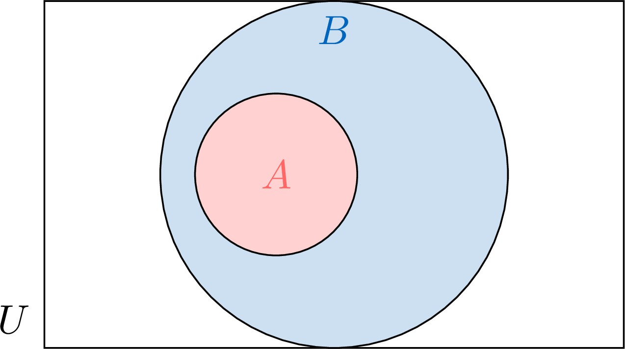

Proof

The event $A$ and its complement $A'$ form the two-piece partition of $U$. The Proposition “Partition Induced on an Event” therefore cuts $B$ into two mutually exclusive pieces, $B \cap A$ and $B \cap A'$: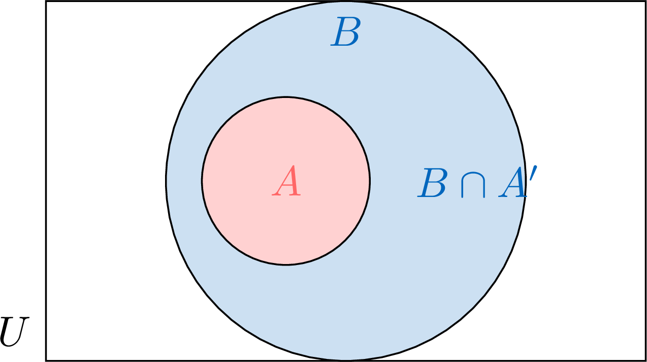

$$\begin{aligned}[t] B &= (B \cap A) \cup (B \cap A') && \text{(the partition $\{A, A'\}$ cuts $B$)}\\ &= A \cup (B \cap A') && \text{($B \cap A = A$, since $A \subseteq B$)} \end{aligned}$$ The two pieces are mutually exclusive, so Axiom 3 applies, and Axiom 1 closes the argument: $$\begin{aligned}[t] P(B) &= P(A) + P(B \cap A') && \text{(Axiom 3)}\\ &\geq P(A) && \text{(Axiom 1: $P(B \cap A') \geq 0$).} \end{aligned}$$ So $A \subseteq B$ implies $P(A) \leq P(B)$. The hypothesis $A \subseteq B$ was used exactly once: to replace $B \cap A$ by $A$.

Proposition — Bounds of a Probability

For any event $E$, $$\textcolor{colorprop}{0 \leq P(E) \leq 1}.$$ A probability is never negative, and never exceeds the probability of the whole sample space.

Proof

The lower bound is Axiom 1. For the upper bound, every event is a part of the sample space, so $E \subseteq U$, and monotonicity applies: $$\begin{aligned}[t] P(E) &\leq P(U) && \text{(monotonicity, since $E \subseteq U$)}\\ &= 1 && \text{(Axiom 2).} \end{aligned}$$

Skills to practice

Applying the Complement Rule

II.3 The Addition Law

Proposition — Addition Law of Probability

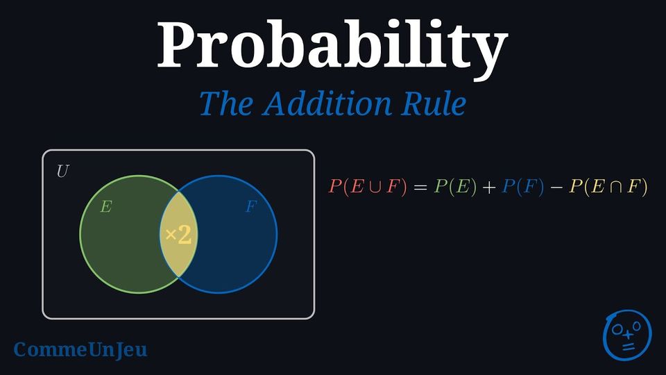
For any two events $E$ and $F$, $$\textcolor{colorprop}{P(E \cup F) = P(E) + P(F) - P(E \cap F)}$$ which can also be written $$\textcolor{colorprop}{P(E \cup F) + P(E \cap F) = P(E) + P(F)}.$$ This formula holds whether or not $E$ and $F$ are mutually exclusive. If they are mutually exclusive, then $P(E \cap F) = 0$ and the formula becomes $P(E \cup F) = P(E) + P(F)$.

Proof

The Venn diagram below shows the sample space $U$ with two intersecting events, $E$ and $F$.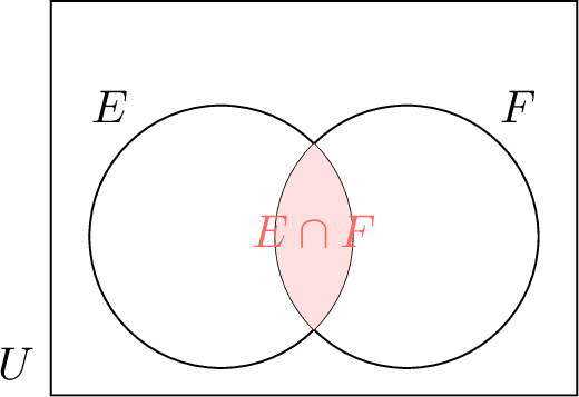

The region represents the event $E \cap F$; its probability $P(E \cap F)$ is counted twice in $P(E) + P(F)$. To correct for this, we must subtract $P(E \cap F)$ once.
Therefore, the total probability of the union is $$P(E \cup F) = P(E) + P(F) - P(E \cap F).$$ The same count, written with events. The union $E \cup F$ is made of the outcomes of $E$ together with the outcomes of $F$ that are not in $E$: $E \cup F = E \cup (F \cap E')$, two events with no outcome in common. In the same way, $F = (F \cap E) \cup (F \cap E')$, two events with no outcome in common, so $P(F) = P(F \cap E) + P(F \cap E')$. Hence $$\begin{aligned}[t] P(E \cup F) &= P(E) + P(F \cap E') && \text{($E$ and $F \cap E'$ have no outcome in common)}\\ &= P(E) + P(F) - P(F \cap E) && \text{($P(F \cap E') = P(F) - P(F \cap E)$)}, \end{aligned}$$ and since $F \cap E = E \cap F$, this is the addition law.

Method — Using the Addition Relation

The relation ties together four quantities: $P(A)$, $P(B)$, $P(A \cap B)$ and $P(A \cup B)$. Knowing three of them always gives the fourth.

Name the two events and translate the sentence: “$A$ or $B$” — possibly both — is $A \cup B$; “$A$ and $B$” is $A \cap B$.
Write down the three known quantities, each as a probability of one of these four events.
Write the relation as a balance: the two sides always weigh the same, $$P(A \cup B) + P(A \cap B) = P(A) + P(B).$$
Isolate the missing quantity by moving the other three to the opposite side.
Check the result: a probability lies between $0$ and $1$, and $P(A \cap B)$ can exceed neither $P(A)$ nor $P(B)$, since the outcomes of $A \cap B$ are among those of $A$, and among those of $B$.

If $A$ and $B$ are mutually exclusive, then $P(A \cap B) = 0$ and the balance becomes $P(A \cup B) = P(A) + P(B)$. Never add two probabilities without first checking that the events cannot happen together.

Example

A school is holding a talent show. One student is chosen at random: the outcomes of this experiment are the students of the school, and $U$ is the set of all of them. Let $S$ be the set of the students who participate in singing and $D$ the set of the students who participate in dancing. The probability that the chosen student participates in singing is $0.4$, the probability that they participate in dancing is $0.3$, and the probability that they participate in both singing and dancing is $0.1$. Find the probability that the chosen student participates in singing or dancing (possibly both).

Answer

The events are the sets $S$ (the students who sing) and $D$ (the students who dance); “singing or dancing” is the event $S \cup D$, and “both” is the event $S \cap D$. We are given:

$P(S) = 0.4$
$P(D) = 0.3$
$P(S \cap D) = 0.1$

The students concerned split into three disjoint parts:

singing only: $P(S) - P(S \cap D) = 0.4 - 0.1 = 0.3$;
dancing only: $P(D) - P(S \cap D) = 0.3 - 0.1 = 0.2$;
both: $P(S \cap D) = 0.1$.

Their sum is $0.3 + 0.2 + 0.1 = 0.6$. The Addition Law of Probability gives the same result directly: $$\begin{aligned} P(S \cup D) &= P(S) + P(D) - P(S \cap D) \\ &= 0.4 + 0.3 - 0.1 \\ &= 0.6. \end{aligned}$$ So there is a $0.6$ (or $60\pourcent$) chance that a randomly selected student participates in at least one of the two activities.

Skills to practice

Calculating the Probability of a Union in Context

III Independent Events and Predictions

III.1 Independent Events

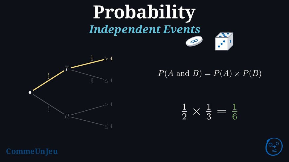
Independent events are events where knowing that one event has happened does not change the probability that the other event happens. For example, when rolling two fair dice at the same time, the result of the first die does not change the chances for the second die — they are independent events.

Report an error

Definition — Independent Events

Two events $A$ and $B$ are independent when the probability that both happen (that is, $P(A\cap B)$ or $P(A \text{ and } B)$) is the product of their individual probabilities. This is called the multiplication rule for independent events: $$P(A \text{ and } B) = P(A) \times P(B)$$

Method — Using a Probability Tree Diagram

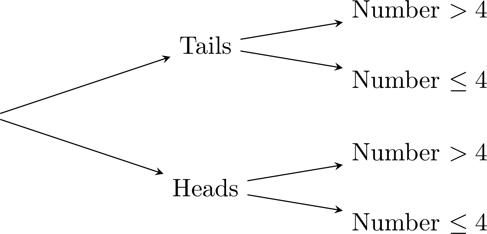
Draw branches for each step: Draw branches for the first event (coin toss) and then, from the end of each of those branches, draw the branches for the second event (die roll).
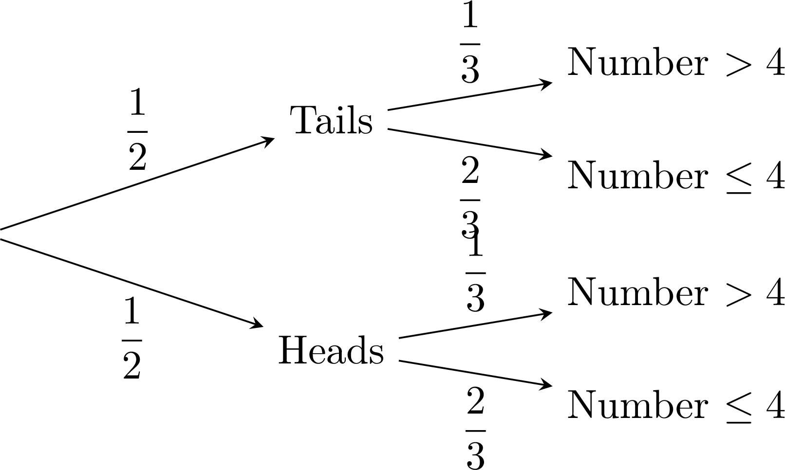
Write probabilities on each branch: The probabilities on the branches from a single point must add up to 1. Because the events are independent, the probabilities on the die-roll branches are the same after “Tails” and after “Heads”.
Multiply along the path: To find the probability of a combined event, multiply the probabilities along the path from start to finish. 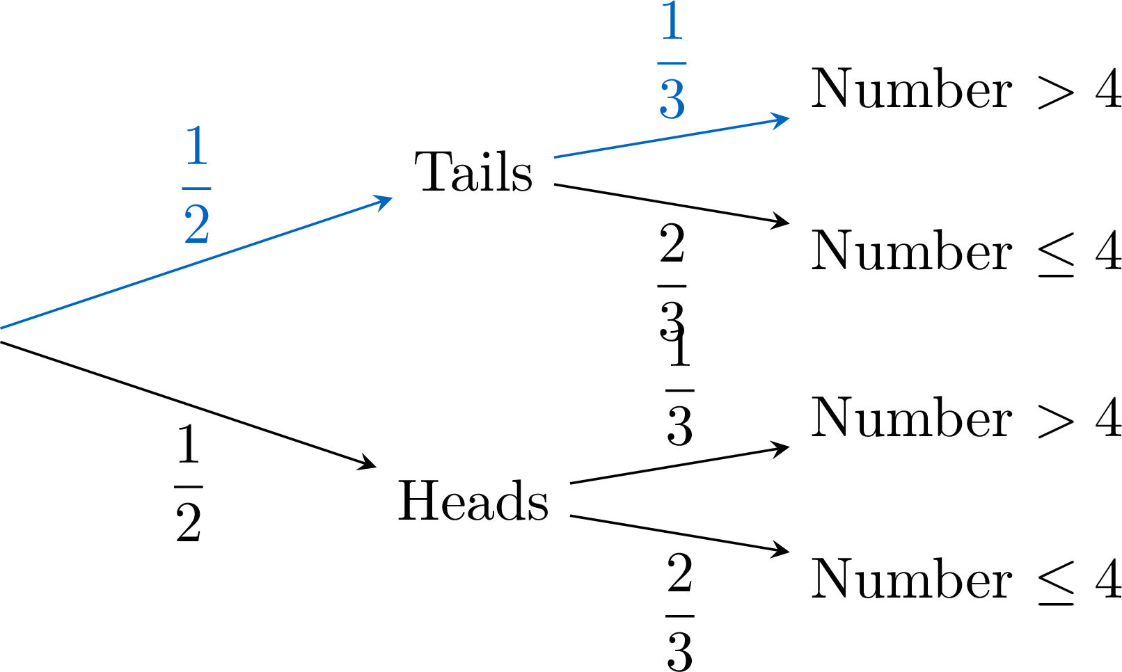$$\textcolor{colorprop}{P(\text{``Tails'' and ``Number > 4''})=\frac{1}{2}\times \frac{1}{3}}$$

Example

A fair coin is tossed, then a fair die is rolled; the two trials are independent. Present the experiment in a table of probabilities and compute the probability of “Tails and an even number”.

Answer

Each row is a result of the coin, each column a result of the die; the margins carry $P(\text{Tails}) = P(\text{Heads}) = \frac{1}{2}$ and $\frac{1}{6}$ for each face. By independence, the probability of a cell is the product of its row total and its column total: $\frac{1}{2} \times \frac{1}{6} = \frac{1}{12}$ for every cell, and the twelve cells add up to $1$.

	$1$	$2$	$3$	$4$	$5$	$6$	Total
Tails	$\frac{1}{12}$	$\frac{1}{12}$	$\frac{1}{12}$	$\frac{1}{12}$	$\frac{1}{12}$	$\frac{1}{12}$	$\frac{1}{2}$
Heads	$\frac{1}{12}$	$\frac{1}{12}$	$\frac{1}{12}$	$\frac{1}{12}$	$\frac{1}{12}$	$\frac{1}{12}$	$\frac{1}{2}$
Total	$\frac{1}{6}$	$\frac{1}{6}$	$\frac{1}{6}$	$\frac{1}{6}$	$\frac{1}{6}$	$\frac{1}{6}$	$1$

“Tails and an even number” is the union of the three cells (Tails, $2$), (Tails, $4$), (Tails, $6$), which are mutually exclusive, so its probability is $3 \times \frac{1}{12} = \frac{1}{4}$. The multiplication rule for independent events gives the same value, $P(\text{Tails}) \times P(\text{even}) = \frac{1}{2} \times \frac{1}{2} = \frac{1}{4}$: the events “Tails” and “even” are independent too. A table cross-classifies the two trials; a tree follows them in order. Both carry the same probabilities.

Skills to practice

Calculating Probabilities on a Tree of Independent Events

III.2 Relative Frequency and Expected Number of Occurrences

Discover

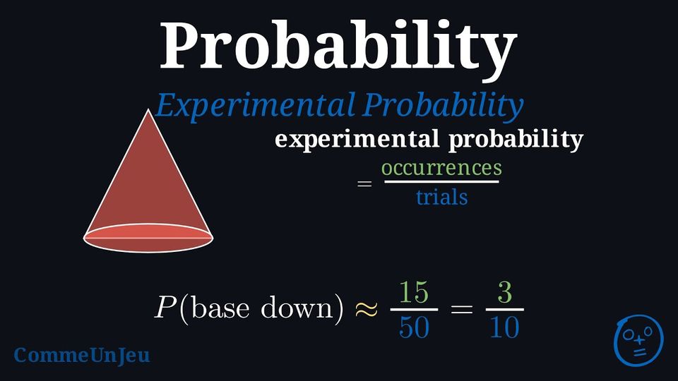
Isaac wants to find the probability that a cone he drops will land on its base. The possible outcomes are “base down” or “on its side”.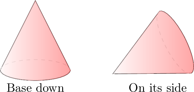

Because of the cone’s shape, these outcomes are not equally likely. A simple theoretical calculation isn’t feasible; the outcomes aren’t symmetric, so Isaac estimates the probability by experiment. He tosses the cone 50 times (50 trials) and records the results:

Base down: 15 times.
On its side: 35 times.

Based on his experiment, Isaac can estimate the probability. The cone landed base down 15 times out of 50: $$ P(\text{base down}) \approx \frac{15}{50} = \frac{3}{10} $$ This result from an experiment is called the experimental probability or relative frequency.

Definition — Experimental Probability (Relative Frequency)

The experimental probability of an event is an estimate found by repeating an experiment many times. It is calculated with the formula: $$ \text{Experimental Probability} = \frac{\text{Number of times an event occurs}}{\text{Total number of trials}} $$ In general, the more trials we do, the closer this frequency tends to get to the true probability.

Proposition — Fluctuation and Stabilisation

An experiment is repeated $n$ times under the same conditions, each repetition having no influence on the others, and the frequency of an event of probability $p$ is observed.

Fluctuation: for a fixed $n$, the frequency can change from one series to another. Two series of the same length do not necessarily give the same frequency.
Stabilisation: when $n$ grows, the frequencies tend to move closer to $p$. Long series usually stray less from $p$ than short ones.
Expected count: over $n$ repetitions, the expected count of the event is $n \times p$; the observed count is about $n \times p$, in the sense that the observed frequency, the count divided by $n$, is usually close to $p$. “About”: the observed count is not known in advance, and it need not equal $n \times p$ exactly.

Example

Two pupils each throw a fair die again and again, and record the frequency of “getting a $6$” as the number $n$ of throws grows.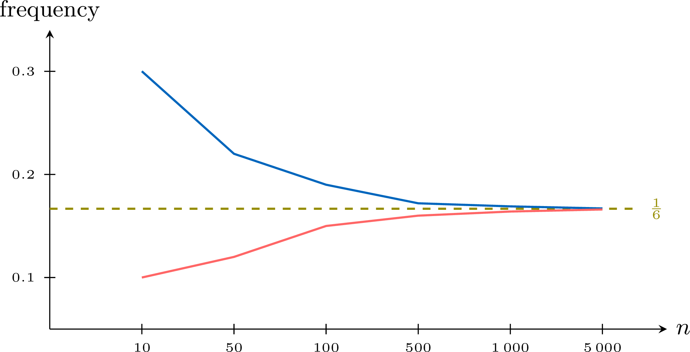

For which values of $n$ do the two frequencies differ the most? What is this phenomenon called?
Around which value do the two curves settle? Why?
How many sixes are expected over $1\,200$ throws?
After $600$ throws, one pupil has only $85$ sixes instead of the $100$ expected. Will the following throws “make up” for it?

Answer

For the small values of $n$: at $n = 10$ the frequencies are $0.30$ and $0.10$. This is the fluctuation: short series differ a lot from one another.
Both curves settle around $\dfrac{1}{6} \approx 0.167$, the probability of getting a $6$ with a fair die. This is the stabilisation: the longer the series, the closer its frequency is to the probability.
$1\,200 \times \dfrac{1}{6} = \textcolor{colordef}{200}$: about $200$ sixes are expected — a real series will give a number close to $200$, without $200$ itself being guaranteed.
No. The die has no memory: each throw still has a probability $\dfrac{1}{6}$ of giving a $6$. The frequency comes close to $\dfrac{1}{6}$ because the $15$ missing sixes weigh less and less among more and more throws — they are diluted, not made up for.

Skills to practice

Calculating an Expected Count

IV Going further

Skills to practice

Making Predictions with Probabilities
Quiz

\(\begin{aligned} & \textcolor{colorprop}{\text{coin 2}} \\ \textcolor{colordef}{\text{coin 1}} \end{aligned} \)	\(\textcolor{colorprop}{H}\)	\(\textcolor{colorprop}{T}\)
\(\textcolor{colordef}{H}\)	\(\textcolor{colordef}{H}\textcolor{colorprop}{H}\)	\(\textcolor{colordef}{H}\textcolor{colorprop}{T}\)
\(\textcolor{colordef}{T}\)	\(\textcolor{colordef}{T}\textcolor{colorprop}{H}\)	\(\textcolor{colordef}{T}\textcolor{colorprop}{T}\)

Notation	Set Vocabulary	Probability Vocabulary	Venn Diagram
\(U\)	Universal set	Sample space
\(x\)	Element of \(U\)	Outcome
\(\emptyset\)	Empty set	Impossible event
\(E\)	Subset of \(U\)	Event
\(x \in E\)	\(x\) is an element of \(E\)	\(x\) is an outcome of \(E\)
\(E'\)	Complement of \(E\) in \(U\)	Complementary event of \(E\)
\(E \cup F\)	Union of \(E\) and \(F\)	\(E\) or \(F\)
\(E \cap F\)	Intersection of \(E\) and \(F\)	\(E\) and \(F\)
\(E \cap F = \emptyset\)	\(E\) and \(F\) are disjoint	\(E\) and \(F\) are mutually exclusive

	\(1\)	\(2\)	\(3\)	\(4\)	\(5\)	\(6\)	Total
Tails	\(\frac{1}{12}\)	\(\frac{1}{12}\)	\(\frac{1}{12}\)	\(\frac{1}{12}\)	\(\frac{1}{12}\)	\(\frac{1}{12}\)	\(\frac{1}{2}\)
Heads	\(\frac{1}{12}\)	\(\frac{1}{12}\)	\(\frac{1}{12}\)	\(\frac{1}{12}\)	\(\frac{1}{12}\)	\(\frac{1}{12}\)	\(\frac{1}{2}\)
Total	\(\frac{1}{6}\)	\(\frac{1}{6}\)	\(\frac{1}{6}\)	\(\frac{1}{6}\)	\(\frac{1}{6}\)	\(\frac{1}{6}\)	\(1\)