International Baccalaureate · DP 2: Applications and Interpretation HL
Coupled Differential Equations
I
Coupled Systems and Equilibrium
I.1
Coupled Systems and Equilibrium Points
A single differential equation describes a single quantity changing over time. However, in the real world, systems often involve multiple variables that interact with one another. For example, the population of predators (like foxes) depends on the population of prey (like rabbits), and vice versa.
These situations are modeled by coupled differential equations. These systems are visualized with phase portraits, solved with matrices, eigenvalues and eigenvectors when they are linear, and approximated with Euler's method.
These situations are modeled by coupled differential equations. These systems are visualized with phase portraits, solved with matrices, eigenvalues and eigenvectors when they are linear, and approximated with Euler's method.
Definition — System of coupled first-order differential equations
A system of coupled first-order differential equations usually takes the form:$$\begin{cases}\dfrac{\mathrm{d}x}{\mathrm{d}t} = f(x, y) \\
\dfrac{\mathrm{d}y}{\mathrm{d}t} = g(x, y)\end{cases}$$ Here, \(t\) is the independent variable (often time), while \(x\) and \(y\) are the dependent variables (state variables).We often denote the time derivatives using dot notation: \(\dot{x} = \dfrac{\mathrm{d}x}{\mathrm{d}t}\) and \(\dot{y} = \dfrac{\mathrm{d}y}{\mathrm{d}t}\).
The system is coupled when the rate of change of at least one variable depends on the other variable (\(f\) depends on \(y\), or \(g\) on \(x\)); otherwise the equations are uncoupled and can be solved independently. The systems considered are autonomous: \(f\) and \(g\) do not depend explicitly on \(t\).
Definition — Equilibrium Points
An equilibrium point is a state where the system does not change. This occurs when both derivatives are zero simultaneously:$$ \frac{\mathrm{d}x}{\mathrm{d}t} = 0 \quad \text{and} \quad \frac{\mathrm{d}y}{\mathrm{d}t} = 0 $$ Example
Consider the system:$$ \frac{\mathrm{d}x}{\mathrm{d}t} = y \quad \text{and} \quad \frac{\mathrm{d}y}{\mathrm{d}t} = -x $$ To find the equilibrium points, we set both derivatives to zero:$$ y = 0 \quad \text{and} \quad -x = 0 $$ The only solution is \((x, y) = (0, 0)\). Thus, the origin is the only equilibrium point.
The Predator–Prey Model
Many coupled systems describe populations that interact. In a predator–prey model (also called the Lotka–Volterra model), \(x\) is the size of a population of prey and \(y\) the size of a population of predators at time \(t\): $$\begin{cases}\dfrac{\mathrm{d}x}{\mathrm{d}t} = ax - bxy \\
\dfrac{\mathrm{d}y}{\mathrm{d}t} = cxy - my\end{cases} \qquad \text{where } a, b, c, m > 0.$$
- \(ax\): without predators, the prey grow exponentially.
- \(-bxy\): the prey are eaten at a rate proportional to the number of meetings between the two species, itself proportional to the product \(xy\).
- \(cxy\): the predators increase thanks to the prey they catch.
- \(-my\): without prey, the predators die out exponentially.
Example — Aphids and Ladybirds
In a greenhouse, the number \(x\) of aphids (in thousands) and the number \(y\) of ladybirds (in hundreds), \(t\) weeks after the start of the observation, are modelled by $$\begin{cases}\dfrac{\mathrm{d}x}{\mathrm{d}t} = 0.6x - 0.03xy \\
\dfrac{\mathrm{d}y}{\mathrm{d}t} = 0.01xy - 0.4y\end{cases}$$ - Find the equilibrium points of the system.
- Interpret each equilibrium point in context.
- An equilibrium point makes both rates zero. Factorising each rate: $$\begin{aligned}[t] 0.6x - 0.03xy = 0 &\iff x(0.6 - 0.03y) = 0 \iff x = 0 \text{ or } y = 20, \\ 0.01xy - 0.4y = 0 &\iff y(0.01x - 0.4) = 0 \iff y = 0 \text{ or } x = 40. \end{aligned}$$ Both conditions must hold together. The choice \(x = 0\) forces \(y = 0\) (since \(x = 40\) is impossible); the choice \(y = 20\) forces \(x = 40\) (since \(y = 0\) is impossible). The equilibrium points are \((0, 0)\) and \((40, 20)\).
- At \((0, 0)\) there are neither aphids nor ladybirds, and nothing changes. At \((40, 20)\), with \(40\,000\) aphids and \(2\,000\) ladybirds, the aphids born each week exactly balance the aphids eaten, and the ladybirds born exactly balance the ladybirds that die: both populations stay constant while the two species live together.
Skills to practice
- Identifying Coupled Systems
- Checking a Solution
- Determining Equilibrium Points
II
Phase Portraits
II.1
Phase Portraits and Trajectories
Definition — Phase Portrait
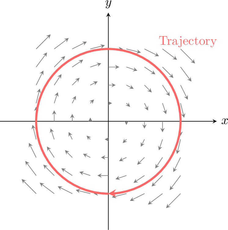
A phase portrait is a graphical representation where: - The axes represent the state variables \(x\) and \(y\) (not \(t\)).
- At each point \((x, y)\), the vector \(\begin{pmatrix} \dot{x} \\ \dot{y} \end{pmatrix}\) indicates the direction and speed of change.
- Trajectories are curves that follow the flow of these vectors, showing how the state of the system evolves over time starting from a specific initial condition.
Example
Consider the system:$$ \frac{\mathrm{d}x}{\mathrm{d}t} = y \quad \text{and} \quad \frac{\mathrm{d}y}{\mathrm{d}t} = -x $$ Let's calculate the velocity vector at a few points: - At \((1, 0)\), vector is \(\begin{pmatrix} 0 \\ -1 \end{pmatrix}\) (Straight down).
- At \((0, -1)\), vector is \(\begin{pmatrix} -1 \\ 0 \end{pmatrix}\) (Straight left).
- At \((-1, 0)\), vector is \(\begin{pmatrix} 0 \\ 1 \end{pmatrix}\) (Straight up).
- At \((0, 1)\), vector is \(\begin{pmatrix} 1 \\ 0 \end{pmatrix}\) (Straight right).
Example — The Predator–Prey Cycle
The aphids \(x\) (in thousands) and the ladybirds \(y\) (in hundreds) of a greenhouse follow the model $$\begin{cases}\dfrac{\mathrm{d}x}{\mathrm{d}t} = 0.6x - 0.03xy \\
\dfrac{\mathrm{d}y}{\mathrm{d}t} = 0.01xy - 0.4y\end{cases}$$ whose equilibrium points are \((0, 0)\) and \((40, 20)\). - Calculate the velocity vector at the points \((60, 20)\), \((40, 30)\), \((20, 20)\) and \((40, 10)\).
- Deduce the sense in which the trajectories turn around the point \((40, 20)\).
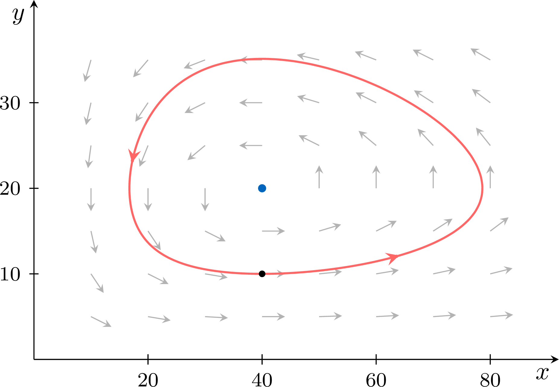
- The phase portrait and the trajectory starting from \((40, 10)\) are shown in the answer. Describe how the two populations evolve from \(40\,000\) aphids and \(1\,000\) ladybirds.
- With \(\dot{x} = 0.6x - 0.03xy\) and \(\dot{y} = 0.01xy - 0.4y\): $$\begin{aligned}[t] (60, 20)&: \ \dot{x} = 36 - 36 = 0, & \dot{y} &= 12 - 8 = 4, \\ (40, 30)&: \ \dot{x} = 24 - 36 = -12, & \dot{y} &= 12 - 12 = 0, \\ (20, 20)&: \ \dot{x} = 12 - 12 = 0, & \dot{y} &= 4 - 8 = -4, \\ (40, 10)&: \ \dot{x} = 24 - 12 = 12, & \dot{y} &= 4 - 4 = 0. \end{aligned}$$ The velocity vectors are \(\begin{pmatrix} 0 \\ 4 \end{pmatrix}\) (upwards), \(\begin{pmatrix} -12 \\ 0 \end{pmatrix}\) (to the left), \(\begin{pmatrix} 0 \\ -4 \end{pmatrix}\) (downwards) and \(\begin{pmatrix} 12 \\ 0 \end{pmatrix}\) (to the right).
- To the right of \((40, 20)\) the motion is upwards, above it to the left, to its left downwards and below it to the right: the trajectories turn anticlockwise around \((40, 20)\).
- The phase portrait, drawn with technology (the arrows give the direction of the velocity):
Skills to practice
- Calculating Velocity Vectors
III
Coupled Linear Systems
III.1
Eigenvalues and Eigenvectors
Recappreviously studied — click to reread
Definition — Eigenvalues and Eigenvectors
Let \(\mathbf{A}\) be a square matrix. An eigenvector of \(\mathbf{A}\) is a non-zero vector \(\mathbf{x}\) such that:$$ \mathbf{A}\mathbf{x} = \lambda \mathbf{x} $$ where \(\lambda\) is a scalar called the eigenvalue associated with the eigenvector \(\mathbf{x}\). Method — Finding Eigenvalues and Eigenvectors
To find the eigenvalues and eigenvectors of a matrix \(\mathbf{A}\): - Find the eigenvalues (\(\lambda\)): Solve the characteristic equation $$ \det(\mathbf{A} - \lambda \mathbf{I}) = 0, $$ where \(\mathbf{I}\) is the identity matrix. The solutions are the eigenvalues.
- Find the eigenvectors (\(\mathbf{x}\)): For each eigenvalue \(\lambda\), substitute it into $$ \mathbf{A}\mathbf{x} = \lambda\mathbf{x}\text{ or } (\mathbf{A} - \lambda \mathbf{I})\mathbf{x} = \mathbf{0} $$ and solve for the non-zero vector \(\mathbf{x}\).
Skills to practice
- Eigenvalues and Eigenvectors
III.2
Solving and Sketching Linear Systems
A fundamental type of coupled system is the linear system with constant coefficients.
These systems can be elegantly solved using matrix algebra. By defining a vector \(\mathbf{x} = \begin{pmatrix} x \\ y \end{pmatrix}\) and a matrix \(\mathbf{A}\), we can condense the system into the compact form \(\dot{\mathbf{x}} = \mathbf{A}\mathbf{x}\).
These systems can be elegantly solved using matrix algebra. By defining a vector \(\mathbf{x} = \begin{pmatrix} x \\ y \end{pmatrix}\) and a matrix \(\mathbf{A}\), we can condense the system into the compact form \(\dot{\mathbf{x}} = \mathbf{A}\mathbf{x}\).
Definition — Coupled Linear Differential Equations
A system of coupled linear differential equations is a set of equations of the form:$$\begin{cases}\dfrac{\mathrm{d}x}{\mathrm{d}t} = ax + by \\
\dfrac{\mathrm{d}y}{\mathrm{d}t} = cx + \mathrm{d}y\end{cases}$$ This can be written in matrix form as:$$ \begin{pmatrix} \dot{x} \\
\dot{y} \end{pmatrix} = \begin{pmatrix} a & b \\
c & d \end{pmatrix} \begin{pmatrix} x \\
y \end{pmatrix} \iff \dot{\mathbf{x}} = \mathbf{A}\mathbf{x} $$ where \(\mathbf{A} = \begin{pmatrix} a & b \\ c & d \end{pmatrix}\) is the matrix of coefficients and \(\mathbf{x} = \begin{pmatrix} x \\ y \end{pmatrix}\) is the state vector. Here \(a, b, c, d\) are constants, with \(b\) or \(c\) non-zero (otherwise the system is uncoupled); such a system, with no forcing term, is called homogeneous.
To find the solution, we look for an analogue to the scalar solution \(x = x_0 e^{kt}\).
If we propose a trial solution of the form \(\mathbf{x} = \mathbf{v}e^{\lambda t}\), differentiating gives \(\dot{\mathbf{x}} = \lambda \mathbf{v}e^{\lambda t}\). Substituting this into the system yields:$$ \lambda \mathbf{v}e^{\lambda t} = \mathbf{A}(\mathbf{v}e^{\lambda t}) \implies \mathbf{A}\mathbf{v} = \lambda \mathbf{v} $$ This equation holds true precisely when \(\lambda\) is an eigenvalue of \(\mathbf{A}\) and \(\mathbf{v}\) is the corresponding eigenvector. Eigenvalues and eigenvectors are computed exactly as when diagonalising a matrix.
If we propose a trial solution of the form \(\mathbf{x} = \mathbf{v}e^{\lambda t}\), differentiating gives \(\dot{\mathbf{x}} = \lambda \mathbf{v}e^{\lambda t}\). Substituting this into the system yields:$$ \lambda \mathbf{v}e^{\lambda t} = \mathbf{A}(\mathbf{v}e^{\lambda t}) \implies \mathbf{A}\mathbf{v} = \lambda \mathbf{v} $$ This equation holds true precisely when \(\lambda\) is an eigenvalue of \(\mathbf{A}\) and \(\mathbf{v}\) is the corresponding eigenvector. Eigenvalues and eigenvectors are computed exactly as when diagonalising a matrix.
Proposition — General Solution using Eigenvalues
Let \(\lambda_1\) and \(\lambda_2\) be the distinct real eigenvalues of matrix \(\mathbf{A}\), with corresponding eigenvectors \(\mathbf{v}_1\) and \(\mathbf{v}_2\). The general solution is:$$ \mathbf{x}(t) = C_1 e^{\lambda_1 t} \mathbf{v}_1 + C_2 e^{\lambda_2 t} \mathbf{v}_2 $$ where \(C_1\) and \(C_2\) are arbitrary constants determined by initial conditions. Example
Solve the system \(\begin{cases} \dfrac{\mathrm{d}x}{\mathrm{d}t} = 4x - 2y \\ \dfrac{\mathrm{d}y}{\mathrm{d}t} = x + y \end{cases}\).
The matrix is \(\mathbf{A} = \begin{pmatrix} 4 & -2 \\ 1 & 1 \end{pmatrix}\).
- Find eigenvalues: $$\begin{aligned} \det(\mathbf{A} - \lambda \mathbf{I}) &= 0\\ (4-\lambda)(1-\lambda) - (-2)(1) &= 0\\ 4 - 5\lambda + \lambda^2 + 2 &= 0\\ \lambda^2 - 5\lambda + 6 &= 0\\ (\lambda - 3)(\lambda - 2) &= 0 \end{aligned}$$ The eigenvalues are \(\lambda_1 = 3\) and \(\lambda_2 = 2\).
- Find eigenvector for \(\lambda_1 = 3\): $$\begin{pmatrix} 4 & -2 \\ 1 & 1 \end{pmatrix} \begin{pmatrix} x \\ y \end{pmatrix} = 3\begin{pmatrix} x \\ y \end{pmatrix} \implies \begin{pmatrix} 1 & -2 \\ 1 & -2 \end{pmatrix} \begin{pmatrix} x \\ y \end{pmatrix} = \begin{pmatrix} 0 \\ 0 \end{pmatrix}$$ \(x - 2y = 0 \implies x = 2y\). Let \(y=1\), then \(x=2\). So \(\mathbf{v}_1 = \begin{pmatrix} 2 \\ 1 \end{pmatrix}\).
- Find eigenvector for \(\lambda_2 = 2\): $$\begin{pmatrix} 4 & -2 \\ 1 & 1 \end{pmatrix} \begin{pmatrix} x \\ y \end{pmatrix} = 2\begin{pmatrix} x \\ y \end{pmatrix} \implies \begin{pmatrix} 2 & -2 \\ 1 & -1 \end{pmatrix} \begin{pmatrix} x \\ y \end{pmatrix} = \begin{pmatrix} 0 \\ 0 \end{pmatrix}$$ \(x - y = 0 \implies x = y\). Let \(y=1\), then \(x=1\). So \(\mathbf{v}_2 = \begin{pmatrix} 1 \\ 1 \end{pmatrix}\).
Proposition — Classification of Equilibrium Points
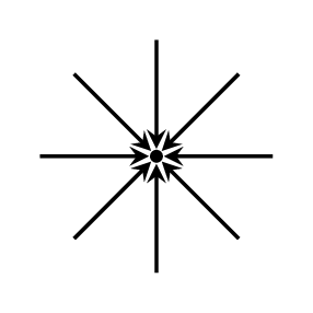
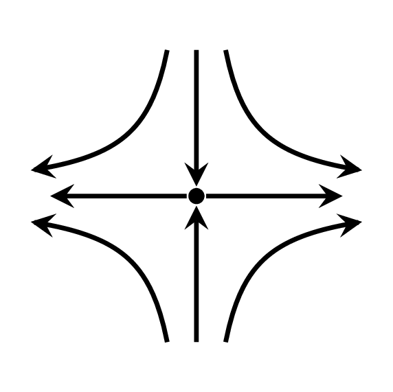
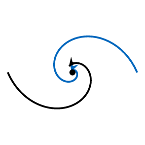
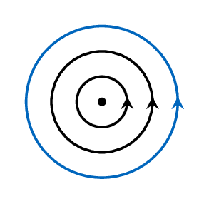
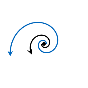
We can describe the behaviour of the phase portrait around an equilibrium point (after translating it to the origin) based on the eigenvalues \(\lambda_1, \lambda_2\) of the system's matrix, assumed non-zero (\(\det \mathbf{A} \neq 0\)). When the eigenvalues form a complex pair \(p \pm qi\), the solutions oscillate, growing or decaying according to the sign of \(p\); such eigenvalues come from the same characteristic equation (via the quadratic formula) and are used here only to classify — no eigenvectors are required. | Stable Node (Sink) | Saddle Point | Unstable Node (Source) |
| {\small \(\lambda_1, \lambda_2 < 0\)} | {\small \(\lambda_1 > 0 > \lambda_2\)} | {\small \(\lambda_1, \lambda_2 > 0\)} |
 |  | 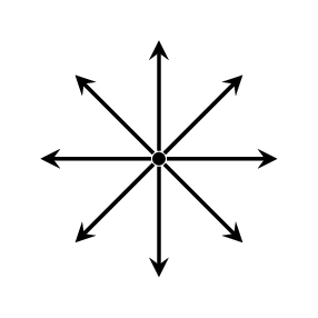 |
| Stable Spiral | Center | Unstable Spiral |
| {\small Complex, Re\((\lambda) < 0\)} | {\small Pure Imaginary} | {\small Complex, Re\((\lambda) > 0\)} |
 |  |  |
Method — Sketching the Phase Portrait of a Linear System
To sketch the phase portrait of \(\dot{\mathbf{x}} = \mathbf{A}\mathbf{x}\), where \(\det \mathbf{A} \neq 0\) (the origin is the only equilibrium point) and the eigenvalues are distinct: - Eigenvalues. Solve \(\det(\mathbf{A} - \lambda\mathbf{I}) = 0\) and name the equilibrium point with the Proposition “Classification of Equilibrium Points”.
- Real eigenvalues: the straight-line trajectories. For each eigenvalue \(\lambda\), find an eigenvector \(\mathbf{v}\) and draw the line through the origin in the direction of \(\mathbf{v}\). A trajectory that starts on this line stays on it, since it is \(\mathbf{x}(t) = Ce^{\lambda t}\mathbf{v}\): it moves away from the origin if \(\lambda > 0\) and towards the origin if \(\lambda < 0\).
- Real eigenvalues \(\lambda_1 > \lambda_2\): the other trajectories. In \(\mathbf{x}(t) = C_1e^{\lambda_1 t}\mathbf{v}_1 + C_2e^{\lambda_2 t}\mathbf{v}_2\) with \(C_1 \neq 0\), the term of the larger eigenvalue \(\lambda_1\) dominates as \(t\) increases, so the trajectory turns towards the line of \(\mathbf{v}_1\) (in the direction of \(\mathbf{v}_1\) or of \(-\mathbf{v}_1\), according to the sign of \(C_1\)). For an unstable node, it becomes parallel to \(\mathbf{v}_1\) far from the origin; for a stable node, it approaches the origin tangent to \(\mathbf{v}_1\); for a saddle point, it comes in along the line of \(\mathbf{v}_2\) and leaves along the line of \(\mathbf{v}_1\), the two lines being asymptotes.
- Complex eigenvalues \(p \pm qi\). No trajectory is a straight line. The sense of rotation is read from the velocity at the point \((1, 0)\), which is the first column of \(\mathbf{A}\): if its second component is positive, the trajectories turn anticlockwise; if it is negative, clockwise. They spiral inwards if \(p < 0\), outwards if \(p > 0\), and are closed curves (ellipses) around the origin if \(p = 0\).
- A trajectory from a given point \(\mathbf{x}_0\) starts in the direction of the velocity \(\mathbf{A}\mathbf{x}_0\), then follows the pattern of steps 2 to 4. Two trajectories never cross.
Example — A Saddle Point and a Particular Solution
Consider the system \(\begin{cases} \dfrac{\mathrm{d}x}{\mathrm{d}t} = x + 2y \\ \dfrac{\mathrm{d}y}{\mathrm{d}t} = 3x + 2y \end{cases}\). - Find the eigenvalues and eigenvectors of the matrix of the system, and name the equilibrium point.
- Find the particular solution with \(x(0) = 3\) and \(y(0) = 2\), and the velocity \(\dot{\mathbf{x}}\) at \(t = 0\).
- Sketch the phase portrait, with the trajectory that starts at \((3, 2)\).
- Describe the long-term behaviour of this particular solution.
- The matrix is \(\mathbf{A} = \begin{pmatrix} 1 & 2 \\ 3 & 2 \end{pmatrix}\) and $$\begin{aligned}[t] \det(\mathbf{A} - \lambda\mathbf{I}) &= (1 - \lambda)(2 - \lambda) - 6 && \text{(determinant)} \\ &= \lambda^2 - 3\lambda - 4 && \text{(expand)} \\ &= (\lambda - 4)(\lambda + 1). && \text{(factorise)} \end{aligned}$$ For \(\lambda_1 = 4\), \((\mathbf{A} - 4\mathbf{I})\mathbf{v} = \mathbf{0}\) gives \(-3x + 2y = 0\): \(\mathbf{v}_1 = \begin{pmatrix} 2 \\ 3 \end{pmatrix}\). For \(\lambda_2 = -1\), \((\mathbf{A} + \mathbf{I})\mathbf{v} = \mathbf{0}\) gives \(2x + 2y = 0\): \(\mathbf{v}_2 = \begin{pmatrix} 1 \\ -1 \end{pmatrix}\). The eigenvalues are real with opposite signs: the origin is a saddle point.
- The general solution is \(\mathbf{x}(t) = C_1e^{4t}\begin{pmatrix} 2 \\ 3 \end{pmatrix} + C_2e^{-t}\begin{pmatrix} 1 \\ -1 \end{pmatrix}\). At \(t = 0\): $$\begin{cases} 2C_1 + C_2 = 3 \\ 3C_1 - C_2 = 2 \end{cases}$$ Adding the equations gives \(5C_1 = 5\), so \(C_1 = 1\) and \(C_2 = 1\): $$x(t) = 2e^{4t} + e^{-t}, \qquad y(t) = 3e^{4t} - e^{-t}.$$ Check: \(x(0) = 3\) and \(y(0) = 2\). At \(t = 0\), \(\dot{\mathbf{x}} = \mathbf{A}\begin{pmatrix} 3 \\ 2 \end{pmatrix} = \begin{pmatrix} 3 + 4 \\ 9 + 4 \end{pmatrix} = \begin{pmatrix} 7 \\ 13 \end{pmatrix}\) (also \(\dot{x}(0) = 8 - 1\) and \(\dot{y}(0) = 12 + 1\)).
- The line \(y = \frac{3}{2}x\) (direction \(\mathbf{v}_1\)) is travelled away from the origin, the line \(y = -x\) (direction \(\mathbf{v}_2\)) towards it. The other trajectories come in along \(y = -x\) and leave along \(y = \frac{3}{2}x\); the trajectory through \((3, 2)\) is drawn thick.
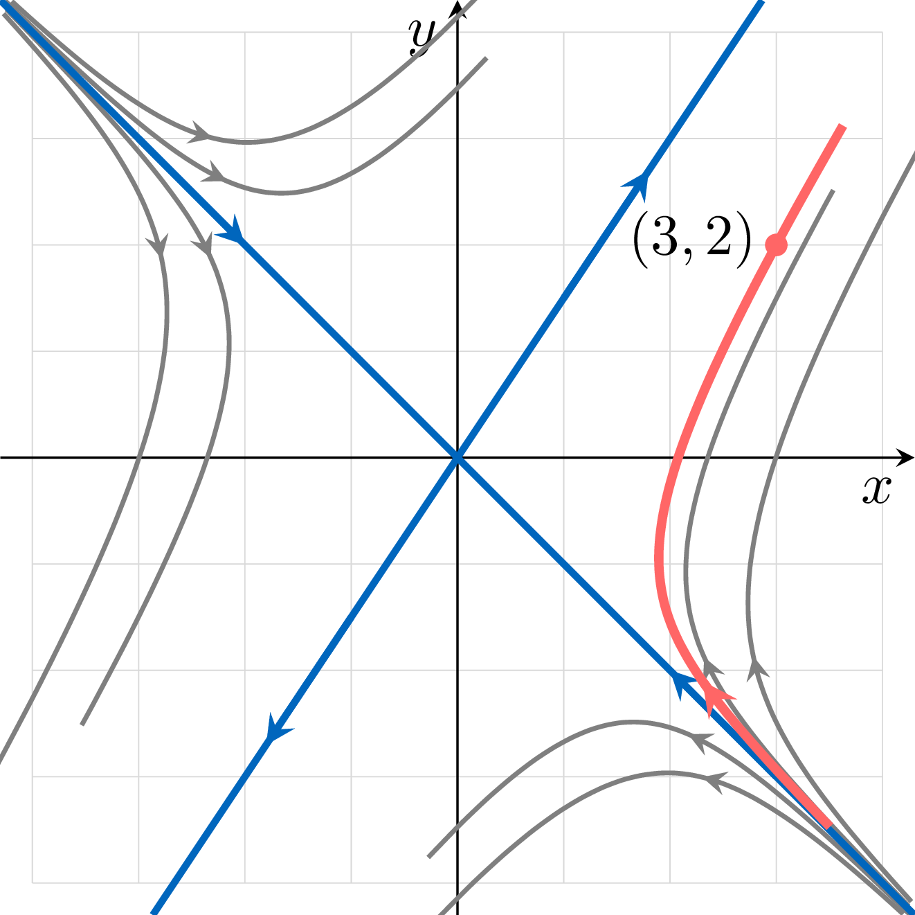
- As \(t \to +\infty\), \(e^{-t} \to 0\), so \(\mathbf{x}(t) \approx e^{4t}\begin{pmatrix} 2 \\ 3 \end{pmatrix}\): \(x\) and \(y\) grow without bound, with \(\dfrac{y}{x} \to \dfrac{3}{2}\). More precisely, \(y - \frac{3}{2}x = -e^{-t} - \frac{3}{2}e^{-t} = -\frac{5}{2}e^{-t} \to 0\): the trajectory approaches the line \(y = \frac{3}{2}x\), which is an asymptote.
Example — A Stable Spiral
Consider the system \(\begin{cases} \dfrac{\mathrm{d}x}{\mathrm{d}t} = x - 2y \\ \dfrac{\mathrm{d}y}{\mathrm{d}t} = 3x - 2y \end{cases}\). - Show that the eigenvalues of the matrix of the system are \(\dfrac{-1 \pm i\sqrt{15}}{2}\), and name the equilibrium point.
- Determine the sense of rotation of the trajectories.
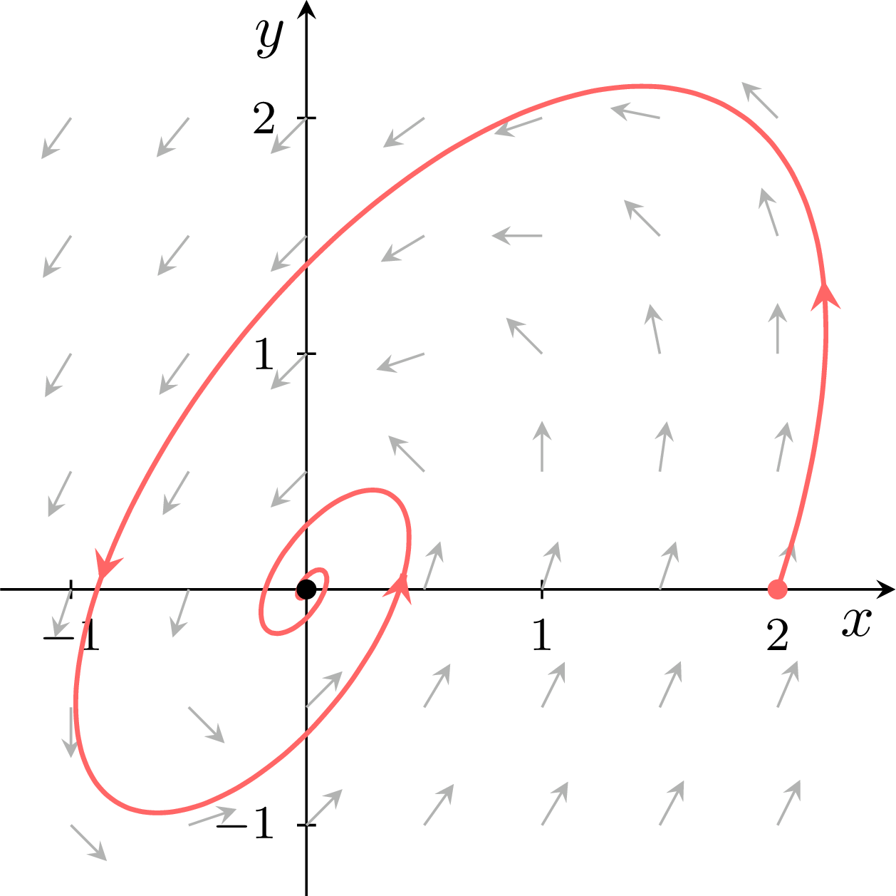
- Sketch the trajectory that starts at \((2, 0)\).
- The matrix is \(\mathbf{A} = \begin{pmatrix} 1 & -2 \\ 3 & -2 \end{pmatrix}\) and $$\begin{aligned}[t] \det(\mathbf{A} - \lambda\mathbf{I}) &= (1 - \lambda)(-2 - \lambda) + 6 && \text{(determinant)} \\ &= \lambda^2 + \lambda + 4. && \text{(expand)} \end{aligned}$$ The discriminant is \(1 - 16 = -15 < 0\), so \(\lambda = \dfrac{-1 \pm i\sqrt{15}}{2}\). These eigenvalues are complex with real part \(-\frac{1}{2} < 0\): the origin is a stable spiral.
- At \((1, 0)\) the velocity is the first column of \(\mathbf{A}\), \(\begin{pmatrix} 1 \\ 3 \end{pmatrix}\): on the positive \(x\)-axis the motion is upwards, so the trajectories turn anticlockwise.
- The trajectory starts at \((2, 0)\) in the direction of \(\mathbf{A}\begin{pmatrix} 2 \\ 0 \end{pmatrix} = \begin{pmatrix} 2 \\ 6 \end{pmatrix}\), turns anticlockwise and spirals inwards to the origin (drawn with technology, with the velocity field):
Skills to practice
- Naming the Equilibrium Point from the Eigenvalues
- Writing Coupled Systems in Matrix Form
- Solving Coupled Linear Systems
- Solving with Initial Conditions
- Classifying Equilibrium Points
- Sketching Phase Portraits
- Sketching Trajectories from Phase Portraits
IV
Second-Order Differential Equations
IV.1
Second-Order Equations as Systems
Second-order differential equations play a crucial role in physics and engineering. Since Newton's Second Law relates force to acceleration (the second derivative of position), these equations naturally describe mechanical vibrations, such as springs, dampers, and pendulums. Similarly, in electronics, they are essential for modeling the behavior of RLC electrical circuits.
Definition — Second-Order Linear Homogeneous Differential Equation
A second-order linear homogeneous differential equation with constant coefficients is an equation of the form:$$ a\frac{d^2x}{\mathrm{d}t^2} + b\frac{\mathrm{d}x}{\mathrm{d}t} + cx = 0 $$ where \(a, b,\) and \(c\) are constants and \(a \neq 0\). - Second-order: The highest derivative is the second derivative.
- Linear: The variable \(x\) and its derivatives appear to the first power and are not multiplied together.
- Homogeneous: The equation equals zero (there is no external forcing term).
Method — Reduction to a System
Any second-order linear homogeneous differential equation of the form$$ a\frac{d^2x}{\mathrm{d}t^2} + b\frac{\mathrm{d}x}{\mathrm{d}t} + cx = 0 $$ can be converted into a system of two first-order equations. - Introduce a new variable \(y = \dfrac{\mathrm{d}x}{\mathrm{d}t}\) (velocity).
- Differentiate \(y\): \(\dfrac{\mathrm{d}y}{\mathrm{d}t} = \dfrac{d^2x}{\mathrm{d}t^2}\).
- Rearrange the original equation: \(\dfrac{\mathrm{d}y}{\mathrm{d}t} = -\frac{c}{a}x - \frac{b}{a}y\).
- Write as a matrix system: $$ \begin{pmatrix} \dfrac{\mathrm{d}x}{\mathrm{d}t} \\ \dfrac{\mathrm{d}y}{\mathrm{d}t} \end{pmatrix} = \begin{pmatrix} 0 & 1 \\ -\frac{c}{a} & -\frac{b}{a} \end{pmatrix} \begin{pmatrix} x \\ y \end{pmatrix} $$
Example
Convert the second-order differential equation \(\dfrac{d^2x}{\mathrm{d}t^2} + 3\dfrac{\mathrm{d}x}{\mathrm{d}t} + 2x = 0\) into a system of coupled first-order equations.
Let \(y = \dfrac{\mathrm{d}x}{\mathrm{d}t}\). Then:$$ \begin{aligned}\dfrac{\mathrm{d}y}{\mathrm{d}t} &= \frac{d}{\mathrm{d}t}\left(\frac{\mathrm{d}x}{\mathrm{d}t}\right) = \frac{d^2x}{\mathrm{d}t^2} \\
\end{aligned} $$ From the original equation, we rearrange to isolate the second derivative:$$ \frac{d^2x}{\mathrm{d}t^2} = -2x - 3\frac{\mathrm{d}x}{\mathrm{d}t} $$ Substituting \(y\) into this expression:$$ \dfrac{\mathrm{d}y}{\mathrm{d}t} = -2x - 3y $$ The system of coupled equations is:$$\begin{cases}\dfrac{\mathrm{d}x}{\mathrm{d}t} = y \\
\dfrac{\mathrm{d}y}{\mathrm{d}t} = -2x - 3y\end{cases}$$
Example — A Damped Spring in the Phase Plane
The displacement \(x\) (in cm) of a mass on a spring, \(t\) seconds after it is released at rest from \(x = 1\), satisfies $$\dfrac{\mathrm{d}^2x}{\mathrm{d}t^2} + 2\dfrac{\mathrm{d}x}{\mathrm{d}t} + 17x = 0.$$ - Write the equation as a coupled system with \(y = \dfrac{\mathrm{d}x}{\mathrm{d}t}\), and give its matrix.
- Find the eigenvalues and name the equilibrium point \((0, 0)\).
- The trajectory from \((1, 0)\) in the plane \((x, y)\) is shown in the answer. Describe the motion of the mass.
- Describe the motion without damping, when \(\dfrac{\mathrm{d}^2x}{\mathrm{d}t^2} + 17x = 0\).
- With \(y = \dfrac{\mathrm{d}x}{\mathrm{d}t}\), \(\dfrac{\mathrm{d}y}{\mathrm{d}t} = \dfrac{\mathrm{d}^2x}{\mathrm{d}t^2} = -17x - 2y\), so $$\begin{cases} \dfrac{\mathrm{d}x}{\mathrm{d}t} = y \\ \dfrac{\mathrm{d}y}{\mathrm{d}t} = -17x - 2y \end{cases} \qquad \mathbf{A} = \begin{pmatrix} 0 & 1 \\ -17 & -2 \end{pmatrix}.$$
- \(\det(\mathbf{A} - \lambda\mathbf{I}) = -\lambda(-2 - \lambda) + 17 = \lambda^2 + 2\lambda + 17\), with discriminant \(4 - 68 = -64\): \(\lambda = \dfrac{-2 \pm 8i}{2} = -1 \pm 4i\). The real part is negative: the origin is a stable spiral. At \((1, 0)\) the velocity is \(\begin{pmatrix} 0 \\ -17 \end{pmatrix}\): the trajectories turn clockwise.
- The trajectory spirals clockwise into the origin:
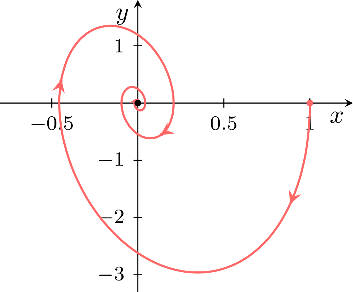
- Without damping, \(\lambda^2 + 17 = 0\) gives \(\lambda = \pm i\sqrt{17}\), purely imaginary: the origin is a centre. The trajectories are closed curves: the mass oscillates forever with the same amplitude.
Skills to practice
- Converting Second-Order Equations to Systems
- Modelling Physical Systems with Second-Order Equations
V
Euler's Method for Coupled Systems
V.1
Euler's Method for One Equation
Recappreviously studied — click to reread
Method — Euler's Method
To approximate the solution to \(\dfrac{\mathrm{d}y}{\mathrm{d}x} = f(x,y)\) with initial condition \((x_0, y_0)\) and a step size \(h\), the coordinates of the next point \((x_{n+1}, y_{n+1})\) are found from the previous point \((x_n, y_n)\) using the iterative formulas: $$ \begin{cases} x_{n+1} = x_n + h, \\
y_{n+1} = y_n + h \cdot f(x_n, y_n). \end{cases} $$ Skills to practice
- Euler's Method for One Equation
V.2
Approximating a Coupled System
When exact solutions are difficult to find (e.g., non-linear systems), we use Euler's method to approximate the trajectory. For a system \(\dfrac{\mathrm{d}x}{\mathrm{d}t} = f(x, y)\) and \(\dfrac{\mathrm{d}y}{\mathrm{d}t} = g(x, y)\) with step size \(h\):
Method — Iterative Formulas
Given initial values \((x_n, y_n)\) at time \(t_n\): - Calculate the slopes: \(m_x = f(x_n, y_n)\) and \(m_y = g(x_n, y_n)\).
- Update the variables: $$ x_{n+1} = x_n + h \cdot m_x $$ $$ y_{n+1} = y_n + h \cdot m_y $$ $$ t_{n+1} = t_n + h $$
Example
Approximate the solution for \(\begin{cases} \dfrac{\mathrm{d}x}{\mathrm{d}t} = x + y \\ \dfrac{\mathrm{d}y}{\mathrm{d}t} = x - y \end{cases}\) with initial condition \(x(0)=1, y(0)=0\) and step size \(h=0.1\). Carry out two steps (to \(t = 0.2\)). - Step 0: \(t_0=0, x_0=1, y_0=0\).
- Step 1: $$ \dfrac{\mathrm{d}x}{\mathrm{d}t}\bigg|_{(1,0)} = 1+0 = 1 \implies x_1 = 1 + 0.1(1) = 1.1 $$ $$ \dfrac{\mathrm{d}y}{\mathrm{d}t}\bigg|_{(1,0)} = 1-0 = 1 \implies y_1 = 0 + 0.1(1) = 0.1 $$
- Step 2: $$ \dfrac{\mathrm{d}x}{\mathrm{d}t}\bigg|_{(1.1,0.1)} = 1.1 + 0.1 = 1.2 \implies x_2 = 1.1 + 0.1(1.2) = 1.22 $$ $$ \dfrac{\mathrm{d}y}{\mathrm{d}t}\bigg|_{(1.1,0.1)} = 1.1 - 0.1 = 1.0 \implies y_2 = 0.1 + 0.1(1.0) = 0.2 $$
Method — Euler's Method for a Coupled System with Technology
The system \(\dfrac{\mathrm{d}x}{\mathrm{d}t} = f(x, y, t)\), \(\dfrac{\mathrm{d}y}{\mathrm{d}t} = g(x, y, t)\) may have rates that also depend on \(t\). It starts from \(t_0\), \(x_0\), \(y_0\), with the step \(h\). A spreadsheet or a graphing calculator repeats the updates and keeps every digit. - Set up the scheme on paper: the number of steps \(n = \dfrac{b - t_0}{h}\) needed to reach \(t = b\) (\(h\) is chosen so that \(n\) is a whole number), and the formulas $$t_{k+1} = t_k + h, \qquad x_{k+1} = x_k + h\,f(x_k, y_k, t_k), \qquad y_{k+1} = y_k + h\,g(x_k, y_k, t_k).$$ Both new values are computed from the values of step \(k\): the new \(x\) is never used in the update of \(y\). A second-order equation \(\dfrac{\mathrm{d}^2x}{\mathrm{d}t^2} = F\left(x, \dfrac{\mathrm{d}x}{\mathrm{d}t}, t\right)\) is first written as the system \(\dfrac{\mathrm{d}x}{\mathrm{d}t} = y\), \(\dfrac{\mathrm{d}y}{\mathrm{d}t} = F(x, y, t)\), as in the Method “Reduction to a System”.
- With a spreadsheet: one row per step, with the columns \(k\), \(t\), \(x\), \(y\). The first row holds \(0\), \(t_0\), \(x_0\), \(y_0\). The next row computes \(t\), \(x\) and \(y\) from the previous row with the three formulas, which are filled down until \(t = b\).
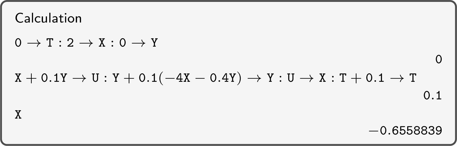
- With a graphing calculator: store \(t_0\), \(x_0\), \(y_0\) in \(T\), \(X\), \(Y\), then type a multiple command that keeps the new value of \(x\) in a spare variable \(U\) while \(Y\) is updated with the old values: \(X + h\,f(X, Y, T) \to U : Y + h\,g(X, Y, T) \to Y : U \to X : T + h \to T\). Each execution performs one step.
- Report the last values to the accuracy asked, rounding only at the end. Written work shows the formulas and the first rows. The approximation generally improves as \(h\) decreases. Comparing the results for \(h\) and for \(\dfrac{h}{2}\) gives an indication of the accuracy: when they agree to the accuracy asked, the estimate can usually be trusted to that accuracy.
| A | B | C | D | |
| 1 | \(k\) | \(t\) | \(x\) | \(y\) |
| 2 | 0 | 0 | 2 | 0 |
| 3 | =A2+1 | =B2+0.1 | =C2+0.1*D2 | =D2+0.1*(-4*C2-0.4*D2) |
| 4 | 2 | 0.2 | 1.92 | -1.568 |
| \(\vdots\) | \(\vdots\) | \(\vdots\) | \(\vdots\) | \(\vdots\) |
| 12 | 10 | 1 | -0.6558839 | -3.6498909 |
Example — Euler's Method for a Damped Spring
A mass on a spring moves with \(\dfrac{\mathrm{d}^2x}{\mathrm{d}t^2} + 0.4\dfrac{\mathrm{d}x}{\mathrm{d}t} + 4x = 0\), where \(x\) is the displacement in cm and \(t\) the time in seconds. It is released at rest from \(x = 2\). - Write the equation as a coupled system.
- Carry out two steps of Euler's method by hand with \(h = 0.1\).
- Use technology to estimate \(x(1)\) with \(h = 0.1\), then with \(h = 0.05\).
- The exact solution gives \(x(1) \approx -0.516\). Comment on the two estimates.
- With \(y = \dfrac{\mathrm{d}x}{\mathrm{d}t}\): \(\dfrac{\mathrm{d}x}{\mathrm{d}t} = y\) and \(\dfrac{\mathrm{d}y}{\mathrm{d}t} = -4x - 0.4y\), with \(x_0 = 2\), \(y_0 = 0\) (released at rest) and \(t_0 = 0\).
- Each step uses the values of the previous step: $$\begin{aligned}[t] x_1 &= x_0 + 0.1\,y_0 = 2 + 0.1 \times 0 = 2, & y_1 &= y_0 + 0.1(-4x_0 - 0.4y_0) = 0 + 0.1 \times (-8) = -0.8, \\ x_2 &= x_1 + 0.1\,y_1 = 2 - 0.08 = 1.92, & y_2 &= y_1 + 0.1(-4x_1 - 0.4y_1) = -0.8 + 0.1 \times (-7.68) = -1.568, \end{aligned}$$ so \(x(0.2) \approx 1.92\) and \(\dfrac{\mathrm{d}x}{\mathrm{d}t}(0.2) \approx -1.568\).
- With \(h = 0.1\), \(n = \dfrac{1}{0.1} = 10\) steps give \(x(1) \approx -0.656\). With \(h = 0.05\), \(n = 20\) steps give \(x(1) \approx -0.593\).
- Both estimates are below \(-0.516\): they overshoot the swing of the mass, by about \(0.140\) and \(0.077\). Halving \(h\) roughly halves the error, but the two estimates differ by \(0.063\): neither can be trusted to one decimal place. On an oscillation, each Euler step shrinks the amplitude less than the true motion does (with \(h = 0.1\) it does not shrink it at all), so the estimated swings are too large and a small step is needed; technology with \(h = 0.01\) gives \(x(1) \approx -0.532\).
Skills to practice
- Applying Euler's Method with Technology
- Applying Euler's Method Step by Step
- Modelling with Coupled Systems
VI
Going further
Skills to practice
- Reasoning and Problem-Solving
- Quiz
Jump to section