International Baccalaureate · DP 2: Applications and Interpretation HL
The Normal Distribution
I
The Normal Distribution
I.1
Continuous Random Variables
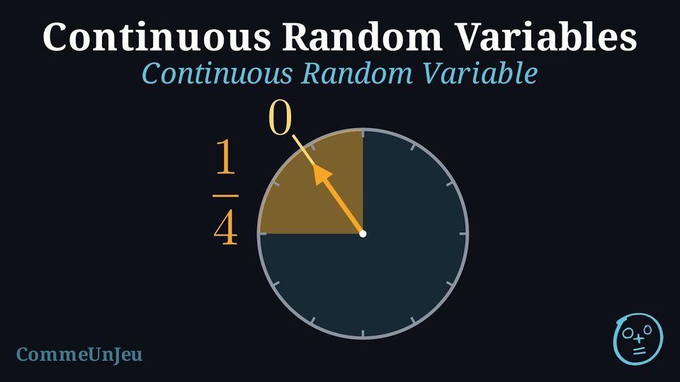
Definition — Continuous Random Variable
A random variable is continuous if its set of possible values is an entire interval of real numbers. A continuous random variable can take any value within its range, meaning there is an infinite number of possibilities. Skills to practice
- Distinguishing Discrete and Continuous Variables
I.2
Normal Curves and Probabilities
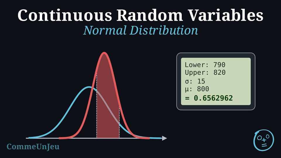
The normal distribution is a key continuous distribution in statistics, often used to model real-world phenomena (e.g., heights, test scores) due to the Central Limit Theorem. This theorem states that the sum or average of many independent random variables, under certain conditions, approximates a normal distribution as the sample size increases. The normal curve is bell-shaped, symmetric, and centred at its mean.
For example, we plot a histogram of the heights of boys at the university. The distribution represented by the histogram follows a bell-shaped curve, also known as a normal distribution. 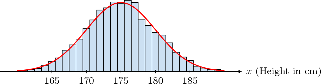
For example, we plot a histogram of the heights of boys at the university. The distribution represented by the histogram follows a bell-shaped curve, also known as a normal distribution.
From a Histogram to a Curve
Record the waiting time, in minutes, of a great many customers at a counter. With classes of width \(5\) minutes, the histogram has a few wide bars; with a larger and larger sample and classes of width \(1\) minute, then \(0.1\) minute, the bars get narrower and their tops draw a curve. This is an idealised model: it assumes that, behind the data, such a curve exists. If the histogram is drawn so that the area of each bar is the frequency of its class, the total area is \(1\), and the frequency of “between \(a\) and \(b\) minutes” is the area of the bars between \(a\) and \(b\). In the limit, the frequency becomes a probability and the bars become the curve of a function \(f\): the probability that the waiting time lies between \(a\) and \(b\) is the area under the curve of \(f\) between \(a\) and \(b\), that is \(\displaystyle\int_a^b f(x)\,\mathrm{d}x\). Such a function, non-negative with total area \(1\), is a probability density; the densities of this chapter are moreover continuous, which is what allows these areas to be computed as integrals. The waiting time is then a random variable with density \(f\), also called a continuous random variable: a variable that can take any real value of an interval, whose probabilities are areas.
Definition — Normal Distribution
A continuous random variable \(X\) follows a normal distribution if its density is:$$f(x) = \frac{1}{\sigma \sqrt{2\pi}} e^{-\frac{1}{2} \left( \frac{x - \mu}{\sigma} \right)^2}, \quad -\infty < x < \infty$$ where \(\mu\) is the mean and \(\sigma^2\) is the variance. The graph is a normal curve (bell-shaped), denoted \(X \sim \mathcal{N}(\mu, \sigma^2)\). 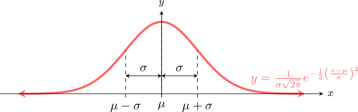
Proposition — Expectation and Variance
For \(X \sim \mathcal{N}(\mu, \sigma^2)\): - \(E(X) = \mu\),
- \(V(X) = \sigma^2\).
Method — Calculating a Normal Probability with Technology
For \(X \sim \mathcal{N}(\mu, \sigma^2)\), the probability of an interval is an area under the normal curve, an integral of the density whose antiderivative cannot be written with the usual functions (polynomials, exponentials, logarithms): the normal cumulative distribution function of a graphing calculator computes it. Its name depends on the model: Normal C.D, normalcdf, normCdf. - State the model: \(X \sim \mathcal{N}(\mu, \sigma^2)\), with its mean \(\mu\) and its standard deviation \(\sigma\) — not the variance \(\sigma^2\): for \(X \sim \mathcal{N}(50, 16)\), \(\sigma = 4\).
- Sketch and shade first: draw a bell curve centred at \(\mu\), mark the bound or bounds, and shade the region of the event. The sketch predicts the size of the answer: a region that contains the mean and most of the curve has a probability close to \(1\), a region that lies on one side of \(\mu\) a probability less than \(0.5\), and a region far in one tail a probability close to \(0\).
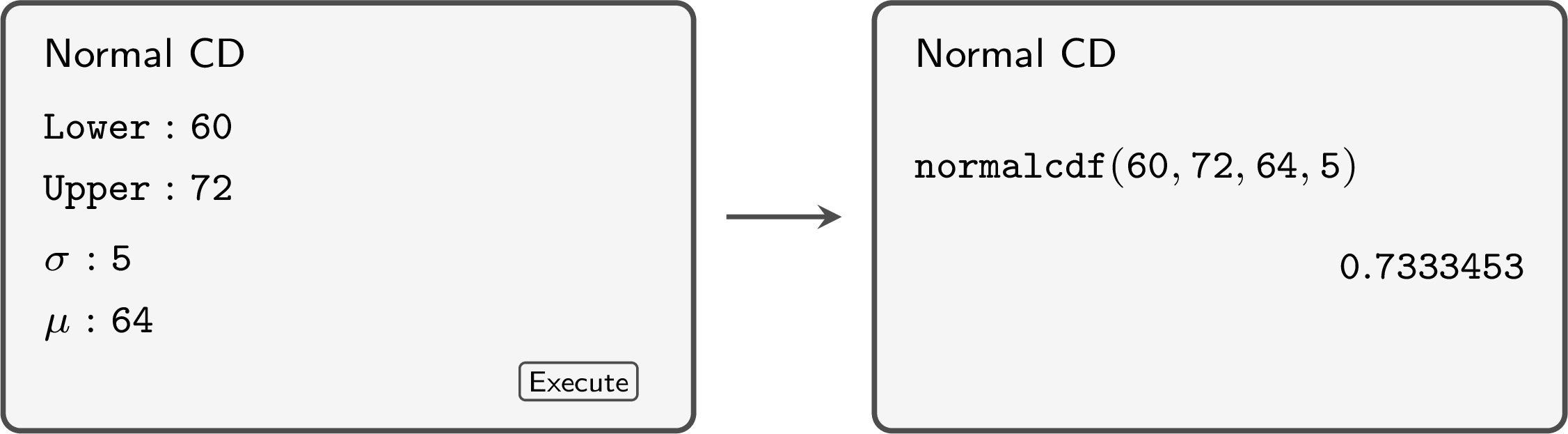
- Enter the bounds of the region, as in the table below, then \(\mu\) and \(\sigma\), each in the field that carries its name: the order of the fields depends on the model, and the command
normalcdftakes the lower bound, the upper bound, \(\mu\), then \(\sigma\). A region with no left end takes as its lower bound a negative number so large that it lies very many standard deviations below the mean, such as \(-10^{99}\), and a region with no right end a positive number as large, such as \(10^{99}\), as its upper bound. - Compare the screen with the sketch, and report the probability to \(3\) significant figures, unless the question asks otherwise.
| Event | Lower bound | Upper bound |
| \(a < X < b\) | \(a\) | \(b\) |
| \(X < b\) | \(-10^{99}\) | \(b\) |
| \(X > a\) | \(a\) | \(10^{99}\) |
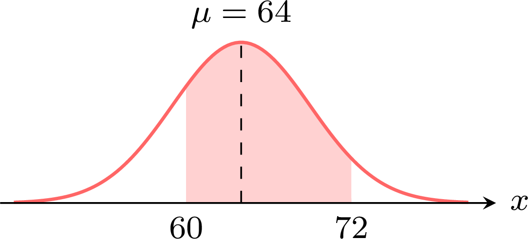
The sketch and the mock-up show the computation of \(P(60 < X < 72)\) for \(X \sim \mathcal{N}(64, 5^2)\): the region contains the mean and most of the curve, and the screen gives \(P(60 < X < 72) \approx 0.733\).
Example
A bakery sells loaves whose mass \(X\), in grams, is normally distributed with mean \(800\) g and standard deviation \(15\) g. Find the probability that a loaf chosen at random has a mass: - between \(790\) g and \(820\) g;
- less than \(780\) g;
- more than \(822\) g.
The model is \(X \sim \mathcal{N}(800, 15^2)\): \(\mu = 800\) and \(\sigma = 15\). The three regions are sketched and shaded first. 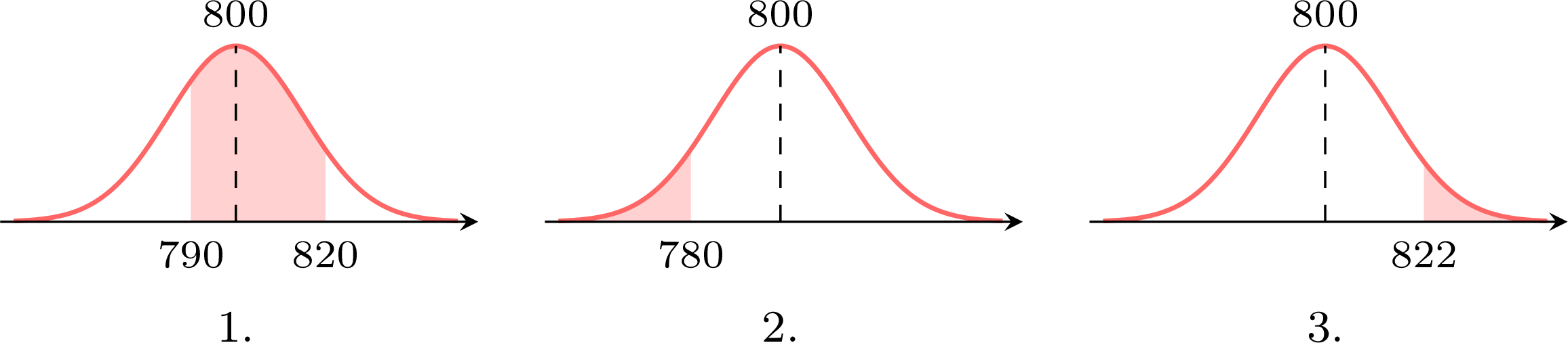
- The region contains the mean and more than half of the curve. With lower bound \(790\), upper bound \(820\), \(\sigma = 15\) and \(\mu = 800\), the screen gives \(0.6562962\): $$P(790 < X < 820) \approx 0.656.$$
- The region is the left tail below \(780\), a small part of the curve. With lower bound \(-10^{99}\) and upper bound \(780\), the screen gives \(0.0912112\): $$P(X < 780) \approx 0.0912.$$
- The region is the right tail above \(822\). With lower bound \(822\) and upper bound \(10^{99}\), the screen gives \(0.0712334\): $$P(X > 822) \approx 0.0712.$$
Example
The battery life \(X\) of a model of phone, in hours, is normally distributed with mean \(14.5\) h and standard deviation \(1.8\) h. - Find \(P(X \geq 12)\).
- A shop sells \(400\) of these phones. Find the expected number of phones whose battery lasts less than \(12\) hours.
- Without technology, find \(P(X \leq 14.5)\).
The model is \(X \sim \mathcal{N}(14.5, 1.8^2)\). 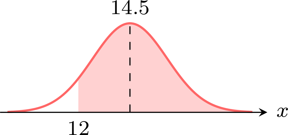
- The region lies to the right of \(12\), which is below the mean: it contains the mean and more than half of the curve, so the probability is greater than \(0.5\). With lower bound \(12\), upper bound \(10^{99}\), \(\sigma = 1.8\) and \(\mu = 14.5\), the screen gives \(0.9175667\): $$P(X \geq 12) \approx 0.918.$$
- A battery lasts less than \(12\) hours with the probability of the complementary event, the unshaded left tail: $$\begin{aligned}[t] P(X < 12) &= 1 - P(X \geq 12) && \text{(complementary event)}\\ &= 1 - 0.9175667\ldots\\ &= 0.0824333\ldots \end{aligned}$$ Each of the \(400\) phones has this probability, so the expected number is $$400 \times P(X < 12) = 400 \times 0.0824333\ldots \approx 32.97.$$ About \(33\) phones are expected to last less than \(12\) hours.
- The normal curve is symmetric about its mean \(\mu = 14.5\), so the area to the left of the mean is half of the total area: $$P(X \leq 14.5) = 0.5.$$
Skills to practice
- Reading and Entering a Normal Model
- Finding Probabilities with Technology
- Counting Expected Numbers with a Normal Model
- Checking Claims with a Normal Model
I.3
The Empirical Rule
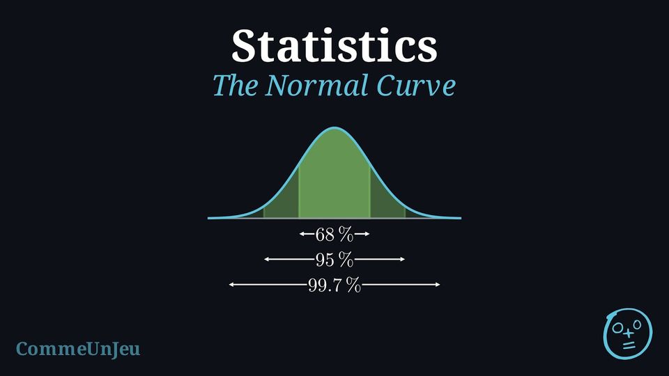
Proposition — Empirical Rule for Normal Distribution
For \(X \sim \mathcal{N}(\mu, \sigma^2)\), the probabilities for intervals centred at the mean are approximately: - \(P(\mu - \sigma \leq X \leq \mu + \sigma) \approx 68.3\pourcent\)
- \(P(\mu - 2\sigma \leq X \leq \mu + 2\sigma) \approx 95.4\pourcent\)
- \(P(\mu - 3\sigma \leq X \leq \mu + 3\sigma) \approx 99.7\pourcent\)
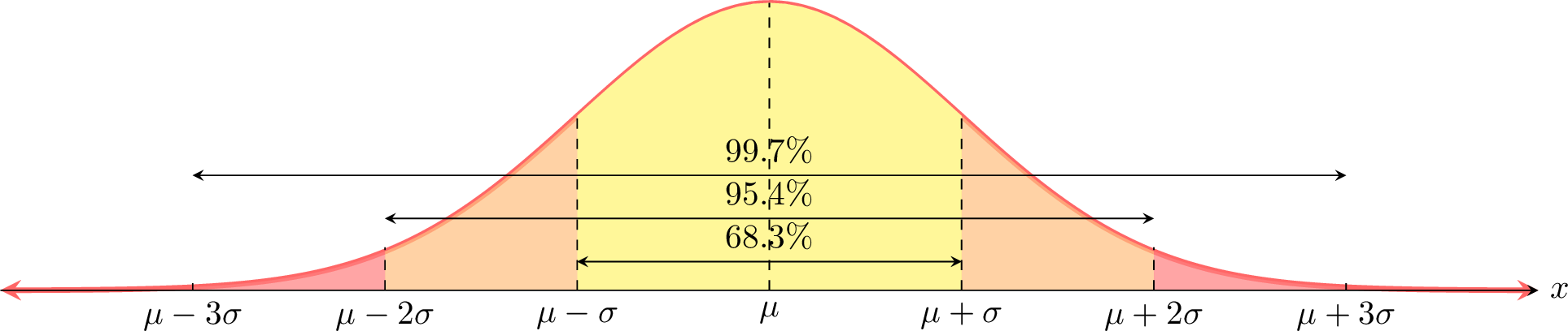
The Empirical Rule states that for a normal distribution, specific percentages of data lie within intervals around the mean. Due to the symmetry of the normal curve, we can break these down to find the probabilities for individual sections, each one standard deviation wide. For example, by symmetry, the area from \(\mu\) to \(\mu+\sigma\) is half of the total area from \(\mu-\sigma\) to \(\mu+\sigma\): $$P(\mu \leq X \leq \mu + \sigma) = \frac{P(\mu - \sigma \leq X \leq \mu + \sigma)}{2} \approx 34.13\pourcent$$ This gives us a detailed map of the normal distribution: 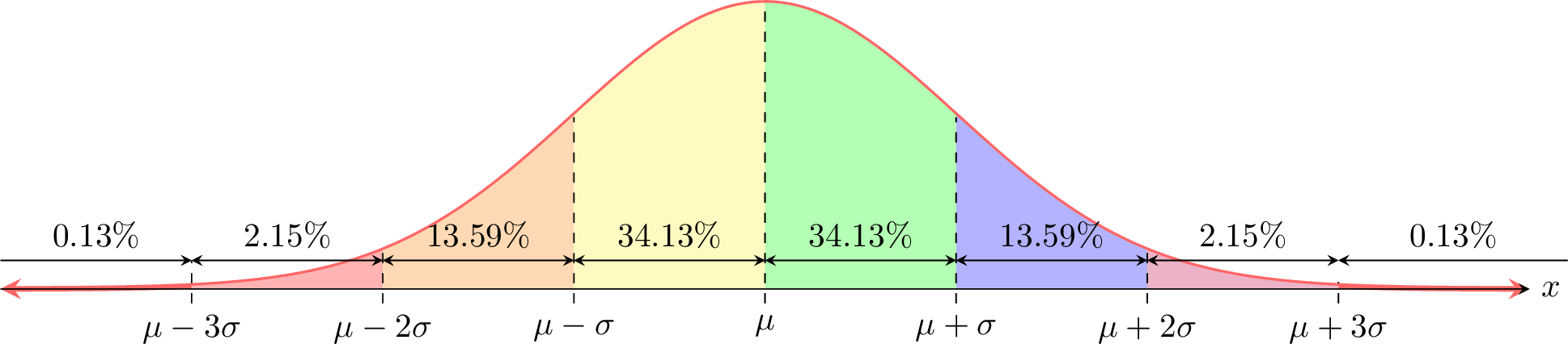
Example
Students’ heights at a school are normally distributed with mean \(\mu = 172 \, \text{cm}\) and standard deviation \(\sigma = 8 \, \text{cm}\). - Find the percentage of students with heights between 164 cm and 172 cm.
- Find the percentage between 164 cm and 180 cm.
- Find the percentage with heights above 196 cm.
- Find the percentage with heights below 196 cm.
- In a group of 500 students, how many are expected to have heights between 164 cm and 180 cm?
First, we label the distribution with the given mean and standard deviation: 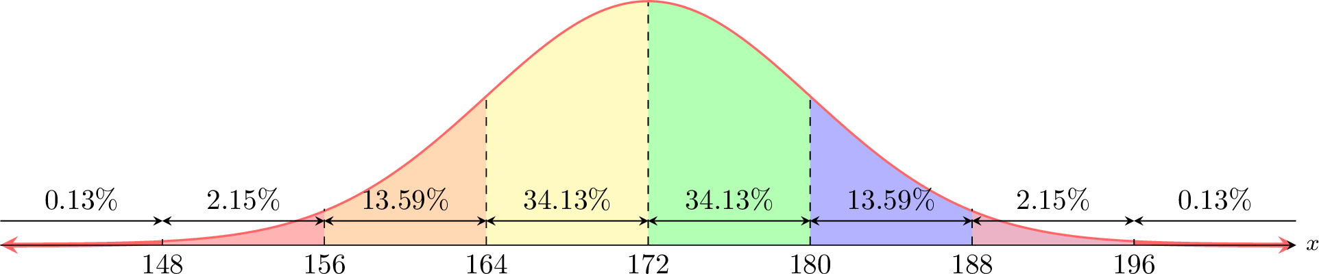
- \(P(164 \leq X \leq 172) = P(\mu - \sigma \leq X \leq \mu) = 34.13\pourcent\).
- \(P(164 \leq X \leq 180) = P(\mu - \sigma \leq X \leq \mu + \sigma) = 34.13\pourcent + 34.13\pourcent = 68.26\pourcent\).
- \(P(X > 196) = P(X \geq \mu + 3\sigma) = 0.13\pourcent\).
- \(P(X < 196) = 1 - P(X \geq 196) = 100\pourcent - 0.13\pourcent = 99.87\pourcent\).
- Expected number = \(68.26\pourcent \times 500 = 0.6826 \times 500 \approx 341\) students.
Skills to practice
- Using the Empirical Rule
I.4
Quantiles and the Inverse Normal
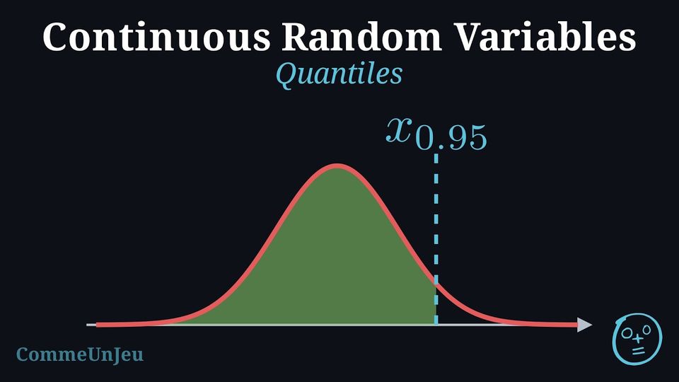
Definition — Quantile
The \(p\)-quantile of a random variable \(X\) is the value \(x_p\) such that \(P(X \leq x_p) = p\). For example, the \(0.95\)-quantile (or 95th percentile) is the value \(x_{0.95}\) below which 95\(\pourcent\) of the distribution's values lie. Method — Finding a Value with the Inverse Normal Function
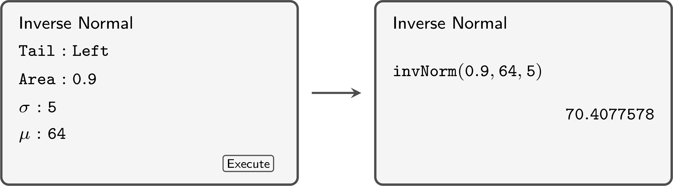
The reverse question gives a probability and asks for a value of \(X\). The inverse normal function of the calculator (Inverse Normal, invNorm) returns the value \(k\) such that \(P(X < k) = p\), for \(0 < p < 1\), from the area \(p\) to the left of \(k\), \(\sigma\) and \(\mu\). - State the model \(X \sim \mathcal{N}(\mu, \sigma^2)\) and name the unknown value \(k\).
- Sketch and shade: place \(k\) on the side of \(\mu\) that the probability indicates — a left area less than \(0.5\) puts \(k\) below the mean — and shade the given area.
- Turn the condition into a left area. The condition \(P(X < k) = p\) is entered as it is; \(P(X > k) = q\) becomes \(P(X < k) = 1 - q\). An interval centred on \(\mu\) that contains the proportion \(p\) of the values leaves \(\frac{1 - p}{2}\) in each tail: its ends are the values with left areas \(\frac{1 - p}{2}\) and \(\frac{1 + p}{2}\).
- Enter the area, \(\mu\) and \(\sigma\), each in its field (the command
invNormtakes the area, \(\mu\), then \(\sigma\); the tail is set to the left, on the models that ask for one), then check the position of \(k\) against the sketch and report it to \(3\) significant figures, or to the precision of the data.
Example
The scores \(X\) on an entrance test are normally distributed with mean \(500\) and standard deviation \(80\). - A scholarship is offered to the top \(12\pourcent\) of the candidates. Find the minimum score for a scholarship.
- The lowest \(5\pourcent\) of the candidates are offered extra support. Find the score below which a candidate is offered support.
The model is \(X \sim \mathcal{N}(500, 80^2)\). 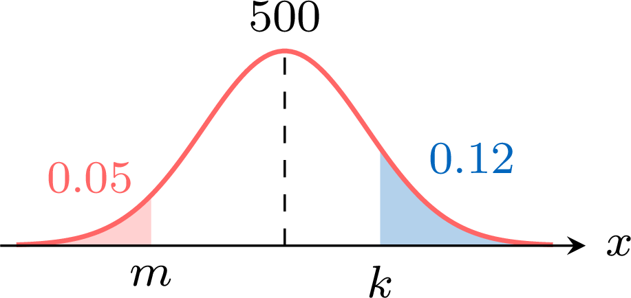
- Let \(k\) be the minimum score: \(P(X > k) = 0.12\). The right tail is small, so \(k\) lies above the mean. As a left area, $$\begin{aligned}[t] P(X < k) &= 1 - P(X > k) && \text{(complementary event)}\\ &= 1 - 0.12\\ &= 0.88. \end{aligned}$$ The inverse normal function with area \(0.88\), \(\sigma = 80\) and \(\mu = 500\) gives \(593.9989\ldots\): the minimum score for a scholarship is about \(594\).
- Let \(m\) be the score: \(P(X < m) = 0.05\), a left tail, so \(m\) lies below the mean. The inverse normal function with area \(0.05\), \(\sigma = 80\) and \(\mu = 500\) gives \(368.4117\ldots\): a candidate who scores below about \(368\) is offered support.
Example
A machine makes bolts whose diameter \(X\), in millimetres, is normally distributed with mean \(10.00\) mm and standard deviation \(0.04\) mm. - Find the interval, centred on the mean, that contains the diameters of \(95\pourcent\) of the bolts. Give its ends to \(3\) decimal places.
- A bolt is rejected when its diameter is less than \(9.93\) mm or more than \(10.07\) mm. Find the proportion of bolts rejected.
The model is \(X \sim \mathcal{N}(10, 0.04^2)\).
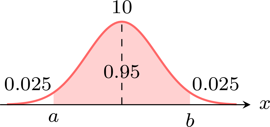
- The central \(95\pourcent\) leaves \(\frac{1 - 0.95}{2} = 0.025\) in each tail. Its ends \(a\) and \(b\) therefore have the left areas \(0.025\) and \(0.975\):
- A bolt is accepted when \(9.93 \leq X \leq 10.07\). With lower bound \(9.93\), upper bound \(10.07\), \(\sigma = 0.04\) and \(\mu = 10\), the normal cumulative distribution function gives \(0.9198817\), so $$\begin{aligned}[t] P(\text{rejected}) &= 1 - P(9.93 \leq X \leq 10.07) && \text{(complementary event)}\\ &= 1 - 0.9198817\ldots\\ &\approx 0.0801. \end{aligned}$$ About \(8.01\pourcent\) of the bolts are rejected. This agrees with question 1: the interval of accepted diameters is narrower than the central interval that holds \(95\pourcent\) of the bolts, so more than \(5\pourcent\) fall outside it.
Skills to practice
- Finding a Value with the Inverse Normal Function
- Setting a Threshold with Percentiles
II
Standard Scores and the Standard Normal Distribution
II.1
Standard Scores
Definition — Variance and Standard Deviation
The variance \(V\) of a data set measures the average of the squared distances of the values from the mean \(\bar{x}\). When the values \(x_i\) have frequencies \(n_i\) (with \(N = \sum n_i\)): $$ V = \frac{1}{N}\sum_{i=1}^{k} n_i (x_i - \bar{x})^2 . $$ The standard deviation \(\sigma\) is the square root of the variance: $$ \sigma = \sqrt{V} = \sqrt{\frac{1}{N}\sum_{i=1}^{k} n_i (x_i - \bar{x})^2} . $$ The variance is expressed in the squared unit of the data, whereas the standard deviation is back in the original unit, which makes it the natural measure of typical distance to the mean. This is the population (descriptive) variance, with denominator \(N\). Definition — Standard Score
The standard score (or \(z\)-score) of an observation \(x\) in a data set whose mean is \(\bar{x}\) and whose standard deviation is \(\sigma > 0\) is: $$ z = \frac{x - \bar{x}}{\sigma} . $$ It rescales the raw value \(x\) by measuring its distance to the mean of its data set, counted in standard deviations.
The standard score states how many standard deviations the observation \(x\) lies from the mean of its data set, and in which direction: \(z>0\) means \(x\) is above the mean, \(z<0\) means below, and the magnitude of \(z\) measures how far. Because \(z\) has no unit, it lets you fairly compare observations coming from different data sets measured on different scales: the larger standard score marks the relatively stronger position within its own set (when a higher raw value indicates a better result).
Example
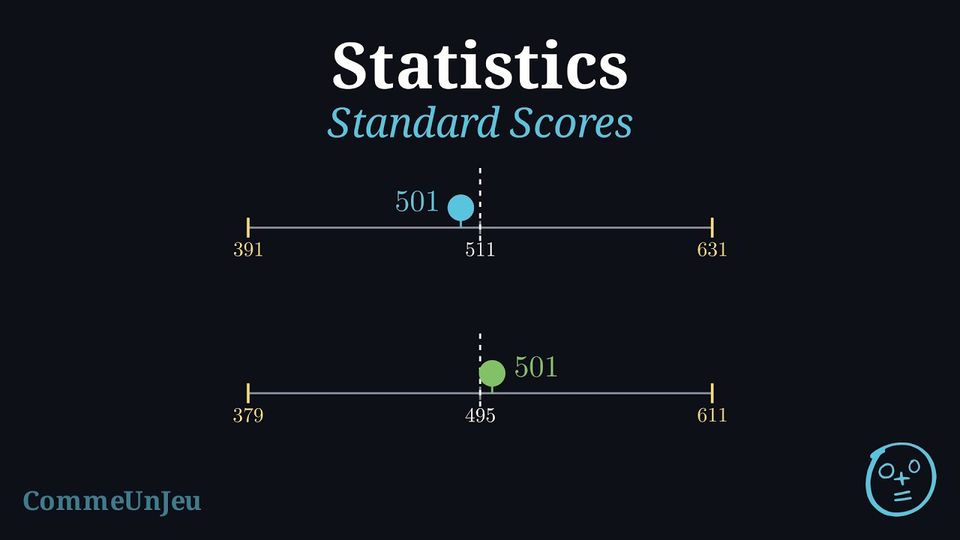
A student sits two tests measured on different scales. On the Mathematics test, the class scores have mean \(\bar{x} = 511\) and standard deviation \(\sigma = 120\). On the Reading test, the class scores have mean \(\bar{x} = 495\) and standard deviation \(\sigma = 116\). The student scores \(501\) on both tests. On which test did the student perform better, relative to the class?
The two raw scores are equal (\(501\)), but each belongs to a different data set, so they are compared through their standard scores. $$ \begin{aligned} z_{\text{Maths}} &= \frac{x - \bar{x}}{\sigma} &&\text{(standard score)} \\
&= \frac{501 - 511}{120} &&\text{(Maths data set)} \\
&\approx -0.083 ; &&\text{(below the mean)} \\
z_{\text{Read}} &= \frac{501 - 495}{116} &&\text{(Reading data set)} \\
&\approx 0.052 . &&\text{(above the mean)} \end{aligned} $$ Although the raw scores are identical, \(z_{\text{Read}} \approx 0.052 > z_{\text{Maths}} \approx -0.083\). The student stands above the mean in Reading but below it in Mathematics, so the student performed better on the Reading test relative to the class.
Skills to practice
- Converting Between Values and Standard Scores
II.2
The Standard Normal Distribution
Definition — Standard Normal Distribution
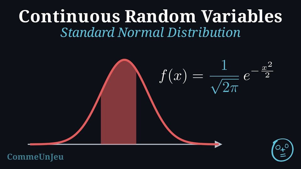
A continuous random variable \(X\) follows a standard normal distribution if it has a mean of 0 and a variance of 1. Its density is:$$f(x) = \frac{1}{\sqrt{2\pi}} e^{-\frac{x^2}{2}}, \quad -\infty < x < \infty$$ This is denoted \(X \sim \mathcal{N}(0, 1)\). 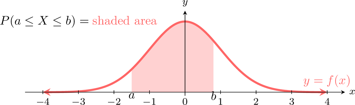
Skills to practice
- Reading Areas under the Standard Normal Curve
III
Choosing and Combining Models
III.1
Choosing a Model: Binomial, Poisson or Normal
Method — Choosing Between the Binomial, Poisson and Normal Models
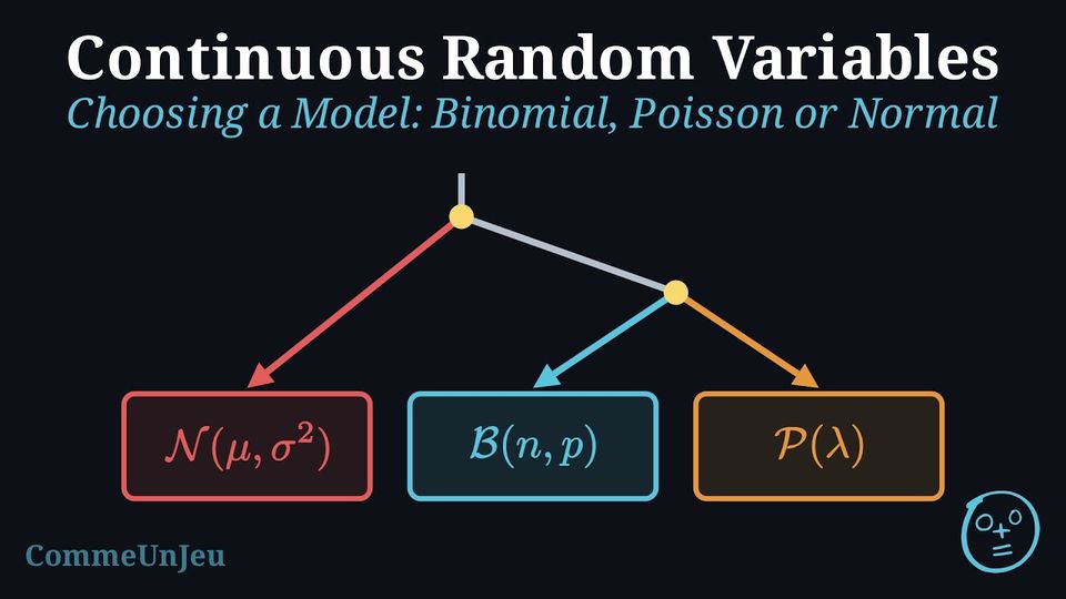
Before any computation, decide what kind of quantity the random variable \(X\) is, then check the conditions of the model. - A measurement or a count? A quantity measured on a continuous scale — a mass, a length, a time, a volume — can take every value of an interval: it calls for a continuous model. A number of successes or of events takes whole values \(0, 1, 2, \dots\): it calls for a discrete model.
- A measurement: the normal model \(\mathcal{N}(\mu, \sigma^2)\) suits values that cluster symmetrically around their mean, fewer and fewer as they move away from it, as in a bell-shaped histogram. Its parameters are the mean \(\mu\) and the standard deviation \(\sigma\).
- A count of successes: the binomial model \(\mathcal{B}(n, p)\) suits the number of successes among a fixed number \(n\) of identical and independent trials, each with the same probability \(p\) of success. The count never exceeds \(n\).
- A count of events: the Poisson model \(\mathcal{P}(\lambda)\) suits the number of events that occur one at a time, independently of one another and at a constant mean rate, in an interval of time or of space; no number of trials is fixed, and the count has no maximum. Its parameter \(\lambda\) is the mean number of events in the interval of the question: a rate given for another interval is first rescaled in proportion.
- Check against the data when they are given: counts whose mean and variance are close support a Poisson model, a binomial count has a variance \(np(1 - p)\) less than its mean \(np\), and values spread roughly symmetrically about their mean support a normal model.
| Random variable | Values | Model | Parameters |
| a measurement | an interval | \(\mathcal{N}(\mu, \sigma^2)\) | \(\mu\) and \(\sigma\) |
| successes among \(n\) trials | \(0, 1, \dots, n\) | \(\mathcal{B}(n, p)\) | \(n\) and \(p\) |
| events in an interval | \(0, 1, 2, \dots\) | \(\mathcal{P}(\lambda)\) | \(\lambda\) |
Example
For each random variable, choose a model, give its parameters and justify the choice, then compute the probability asked. - A typist makes on average \(9\) errors in \(5\) pages, the errors occurring independently of one another and at a constant rate. \(X\) is the number of errors on one page: find \(P(X = 0)\).
- \(4\pourcent\) of the phones made by a factory are faulty, independently of one another. \(Y\) is the number of faulty phones among \(20\) phones chosen at random: find \(P(Y \geq 1)\).
- The times \(T\), in minutes, that a technician takes to repair a phone cluster symmetrically around a mean of \(35\) minutes, in a bell shape, with a standard deviation of \(6\) minutes: find \(P(T < 30)\).
- \(X\) counts events, the errors, in an interval, one page; they occur independently and at a constant rate, and no number of trials is fixed: a Poisson model. The mean on one page is \(\lambda = \frac{9}{5} = 1.8\), so \(X \sim \mathcal{P}(1.8)\) and $$\begin{aligned}[t] P(X = 0) &= \frac{e^{-1.8} \times 1.8^0}{0!} && \text{(Poisson distribution)}\\ &= e^{-1.8}\\ &\approx 0.165. \end{aligned}$$
- \(Y\) counts successes, the faulty phones, among a fixed number \(n = 20\) of phones chosen at random, each faulty with the same probability \(p = 0.04\), independently: \(Y \sim \mathcal{B}(20, 0.04)\). The event “at least one” is the complement of “none”: $$\begin{aligned}[t] P(Y \geq 1) &= 1 - P(Y = 0) && \text{(complementary event)}\\ &= 1 - 0.96^{20}\\ &\approx 0.558. \end{aligned}$$
- \(T\) is a measurement, a time, whose values form a bell shape symmetric about the mean: \(T \sim \mathcal{N}(35, 6^2)\). The region \(T < 30\) is a left tail, below the mean. With lower bound \(-10^{99}\), upper bound \(30\), \(\sigma = 6\) and \(\mu = 35\), the normal cumulative distribution function gives \(0.2023283\ldots\), so \(P(T < 30) \approx 0.202\).
Method — Counting Successes Defined by a Normal Model
A measurement often decides whether an item is a success: a loaf is underweight when its mass is less than a given value, an athlete qualifies when a jump is longer than a given length. Counting such items among \(n\) combines two models. - One item: compute the probability of success \(p\) with the normal model, for example \(p = P(X > a)\) with the normal cumulative distribution function, and keep \(p\) unrounded in the memory of the calculator.
- Several items: when the measurements of the \(n\) items all follow this normal model and are independent, each item is a success with the same probability \(p\), independently of the others, so the number \(Y\) of successes follows the binomial distribution \(\mathcal{B}(n, p)\).
- Compute with the binomial model: \(P(Y = k) = \binom{n}{k}p^k(1 - p)^{n - k}\); for “at least one”, the complementary event gives \(P(Y \geq 1) = 1 - (1 - p)^n\); the binomial functions of the calculator give the other events.
- Round only at the end: a rounded value of \(p\), raised to a power, changes the last significant figures of the answer.
Example
The mass \(X\), in grams, of the eggs of a farm is normally distributed with mean \(62\) g and standard deviation \(4\) g. An egg is sold as large when its mass is more than \(67\) g. A box holds \(6\) eggs chosen at random, whose masses are independent. - Find the probability that an egg is large.
- Find the probability that a box holds exactly \(2\) large eggs.
- Find the probability that a box holds at least one large egg.
- The model of one mass is \(X \sim \mathcal{N}(62, 4^2)\), and an egg is large when \(X > 67\), a right tail. With lower bound \(67\), upper bound \(10^{99}\), \(\sigma = 4\) and \(\mu = 62\), the normal cumulative distribution function gives \(p = P(X > 67) = 0.1056497\ldots\), so \(p \approx 0.106\).
- Let \(Y\) be the number of large eggs in a box. The masses of the \(6\) eggs all follow the model of question 1 and are independent, so each egg is large with the same probability \(p\), independently of the others: \(Y \sim \mathcal{B}(6, p)\) with \(p = 0.1056497\ldots\) kept in memory. Then $$\begin{aligned}[t] P(Y = 2) &= \binom{6}{2}p^2(1 - p)^4 && \text{(binomial distribution)}\\ &= 15 \times 0.1056497\ldots^2 \times 0.8943502\ldots^4\\ &\approx 0.107. \end{aligned}$$
- The event “at least one large egg” is the complement of “no large egg”: $$\begin{aligned}[t] P(Y \geq 1) &= 1 - P(Y = 0) && \text{(complementary event)}\\ &= 1 - (1 - p)^6\\ &= 1 - 0.8943502\ldots^6\\ &\approx 0.488. \end{aligned}$$ With \(p\) rounded to \(0.106\) before the power, the same computation gives \(1 - 0.894^6 \approx 0.489\): the third significant figure changes, which is why \(p\) is rounded only at the end.
Skills to practice
- Choosing the Model of a Random Variable
- Counting Successes Defined by a Normal Model
IV
Going further
Skills to practice
- Problems: Working with Normal Models
- Quiz
Jump to section