International Baccalaureate · MYP 4

Box Plots and Comparing Data Sets

⌚ ~122 min ▢ 13 blocks ✓ 66 exercises ➣ Prerequisites : Statistics: Sampling, Spread and Cumulative Frequency

I Box Plots and Outliers

I.1 Box Plots

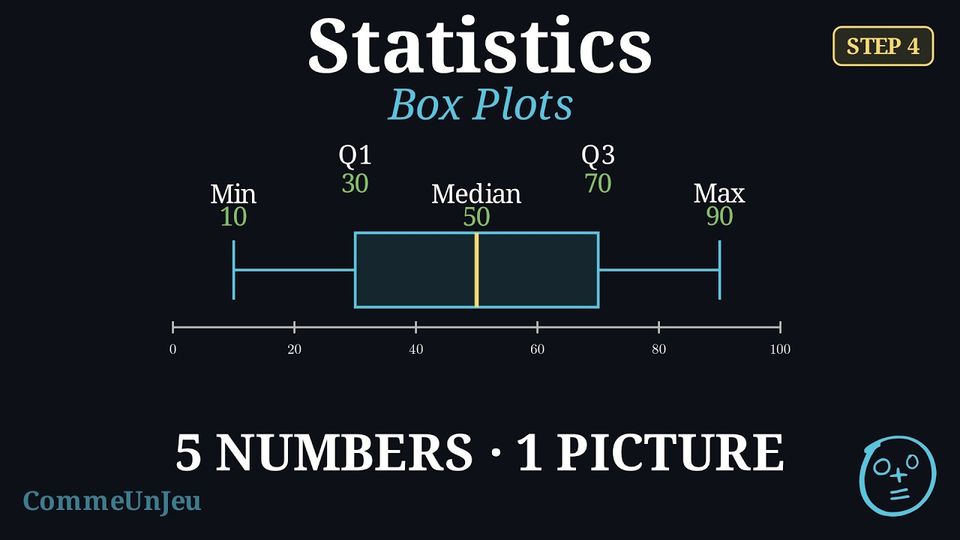
While measures like the mean and the range are useful, they do not give a full picture of the data's distribution. A box plot (or box-and-whisker plot) is a visual tool that summarises a dataset by showing both its centre and its spread simultaneously.

Report an error

Definition — Box Plot

A box plot visually displays the five-number summary above a number line.

A central box is drawn from the lower quartile (Q1) to the upper quartile (Q3).
A line inside the box marks the median (Q2).
Whiskers (lines) extend from the box out to the minimum and maximum values.

The box, drawn from $Q_1$ to $Q_3$, contains at least half of the data — the central half; the line inside shows the centre, and the whiskers show the full range (when there is no outlier).

Method — Constructing a Box Plot

Order the data from least to greatest.
Find the five-number summary: Calculate the minimum, Q1, median, Q3, and maximum.
Draw a number line that covers the full range of your data.
Draw the box and median: Draw a box from Q1 to Q3 and a vertical line inside the box at the median.
Draw the whiskers: Draw lines from the box to the minimum and maximum values.

Example

This box plot shows the number of minutes passengers spent waiting in an airport departure lounge.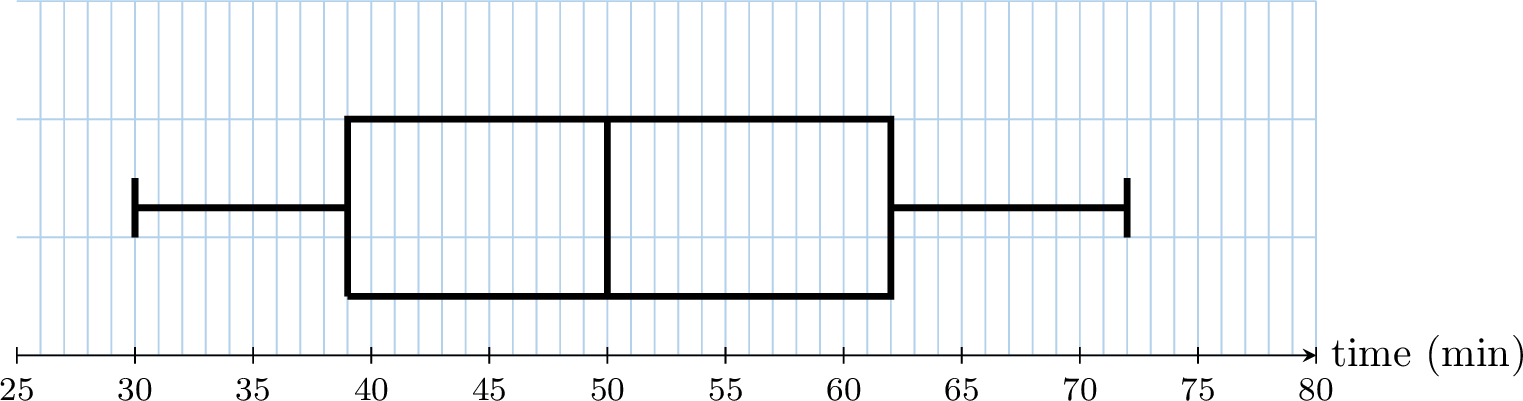

Based on the plot, find the median, the range, and the two quartiles $Q_1$ and $Q_3$.

Answer

By reading the five-number summary from the plot:

Median (Q2): The line inside the box is at 50 minutes.
Range: Maximum - Minimum = $72 - 30 = \textbf{42}$ minutes.
Quartiles: the box runs from $Q_1 = \textbf{39}$ to $Q_3 = \textbf{62}$ minutes.

Skills to practice

Reading and Matching Box Plots

I.2 Outliers

Discover

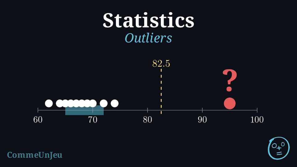
The eleven members of an athletics club ran a $400$ m race. Their times, in seconds and in increasing order, are: $$62,\ 64,\ 65,\ 66,\ 67,\ 68,\ 69,\ 70,\ 72,\ 74,\ 95.$$ The time $95$ s stands apart from the others.
Is $95$ s an unusual time for this club, or simply the slowest one? And $74$ s? Two people looking at the list may disagree: what yardstick could a rule use, so that everyone decides the same way?

Answer

The yardstick is the width of the central half of the data: the interquartile range. With $N = 11$ times, the median is the $6^{\text{th}}$ ordered value, $68$. The lower half $62, \ldots, 67$ and the upper half $69, \ldots, 95$ hold five values each, and their medians are $Q_1 = 65$ and $Q_3 = 72$ (the convention of quartiles as values of the dataset gives the same values), so $\text{IQR} = 72 - 65 = 7$. The usual rule looks one and a half interquartile ranges beyond each quartile: $$\begin{aligned}[t] Q_3 + 1.5 \times \text{IQR} &= 72 + 1.5 \times 7 && \text{(}1.5\text{ IQR above } Q_3\text{)}\\ &= 72 + 10.5\\ &= 82.5, \\ Q_1 - 1.5 \times \text{IQR} &= 65 - 10.5 && \text{(}1.5\text{ IQR below } Q_1\text{)}\\ &= 54.5. \end{aligned}$$ The time $95$ s lies beyond $82.5$ s: it is unusual for this club, an outlier. The time $74$ s lies below $82.5$ s: it is simply the second slowest time. No time lies below $54.5$ s.

Definition — Fences and Outliers

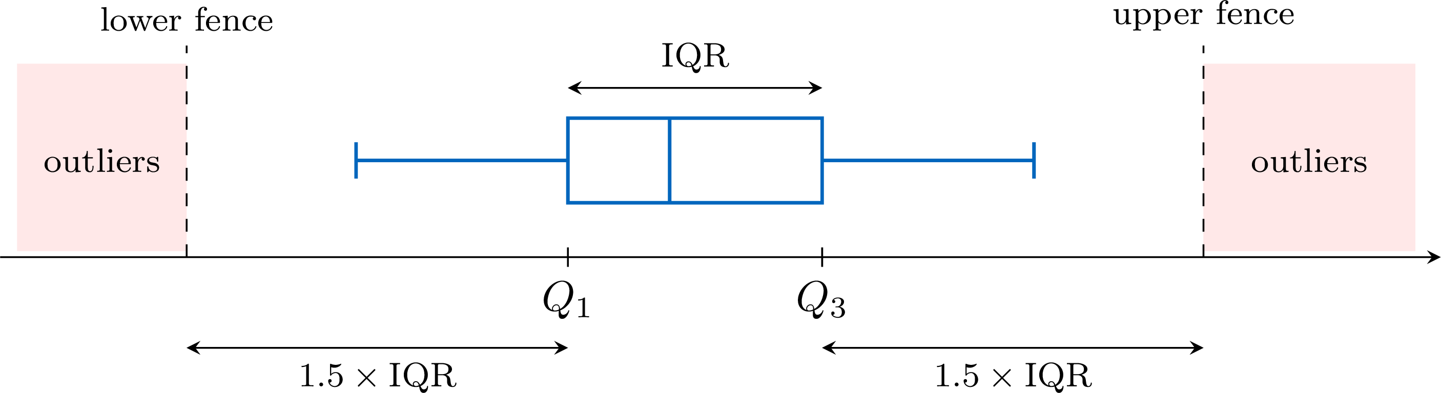
Consider a dataset with lower quartile $Q_1$, upper quartile $Q_3$ and interquartile range $\text{IQR} = Q_3 - Q_1$.

The lower fence is $Q_1 - 1.5 \times \text{IQR}$.
The upper fence is $Q_3 + 1.5 \times \text{IQR}$.

A value of the dataset is an outlier when it lies strictly below the lower fence or strictly above the upper fence. The fences are also called the lower and upper boundaries.

An outlier lies unusually far from the central half of the data. It is not necessarily a mistake: it is a value to check.

Method — Testing Data for Outliers

Find the quartiles: order the data, then find $Q_1$ and $Q_3$ as the medians of the two halves (the median left out when the number of values is odd).
Compute the yardstick: $\text{IQR} = Q_3 - Q_1$, then $1.5 \times \text{IQR}$.
Compute the two fences: $Q_1 - 1.5 \times \text{IQR}$ and $Q_3 + 1.5 \times \text{IQR}$.
Compare the extreme values with the fences: the smallest values with the lower fence, the largest ones with the upper fence. Every value strictly beyond a fence is an outlier; a value equal to a fence is not.
Interpret in context: a recording error is corrected, or removed if the true value is unknown; a genuine value is kept and reported.

Example

Over $15$ working days, a small office recorded the number of emails it received each day. In increasing order: $$12,\ 18,\ 19,\ 21,\ 22,\ 23,\ 24,\ 25,\ 26,\ 27,\ 28,\ 30,\ 31,\ 33,\ 48.$$ Test these data for outliers.

Answer

Quartiles. With $N = 15$ values, the median is the $8^{\text{th}}$ ordered value, $25$. The two halves, $12, \ldots, 24$ and $26, \ldots, 48$, hold seven values each, and their medians are their $4^{\text{th}}$ values: $Q_1 = 21$ and $Q_3 = 30$ (the convention of quartiles as values of the dataset gives the same values).
Yardstick. $\text{IQR} = Q_3 - Q_1 = 30 - 21 = 9$, so $1.5 \times \text{IQR} = 1.5 \times 9 = 13.5$.
Fences. $$\begin{aligned}[t] \text{lower fence} &= Q_1 - 1.5 \times \text{IQR} && \text{(definition)}\\ &= 21 - 13.5 && \text{(}Q_1 = 21\text{)}\\ &= 7.5,\\ \text{upper fence} &= Q_3 + 1.5 \times \text{IQR} && \text{(definition)}\\ &= 30 + 13.5 && \text{(}Q_3 = 30\text{)}\\ &= 43.5. \end{aligned}$$ Comparison. The smallest value, $12$, is above $7.5$: there is no outlier on the low side, even though $12$ is well below the other values. The largest value, $48$, is above $43.5$: it is an outlier; the next one, $33$, is not.
Conclusion. The only outlier is the day with $48$ emails. It is a day to look into (a mailing campaign, a failure of the mail server the day before), not a value to delete automatically.

Method — Drawing a Box Plot with Outliers

When a dataset has outliers, its box plot shows them apart from the other values.

Draw the box and the median line from $Q_1$ to $Q_3$, as usual.
Stop each whisker at the most extreme value that is not an outlier.
Mark each outlier with a cross $\times$ at its value.

The whiskers then show the spread of the ordinary values, and the crosses the values that stand apart.

Example

The numbers of emails received by an office over $15$ working days are, in increasing order: $$12,\ 18,\ 19,\ 21,\ 22,\ 23,\ 24,\ 25,\ 26,\ 27,\ 28,\ 30,\ 31,\ 33,\ 48.$$ Their quartiles are $Q_1 = 21$ and $Q_3 = 30$, and their only outlier is $48$. Draw their box plot, with the outlier marked.

Answer

The median is the $8^{\text{th}}$ of the $15$ ordered values: $25$. The box runs from $Q_1 = 21$ to $Q_3 = 30$, with the median line at $25$. The left whisker goes down to $12$, which is not an outlier. The right whisker stops at $33$, the largest value that is not an outlier, and $48$ is marked by a cross.

Drawn to $48$, the right whisker would hide the gap between $33$ and $48$: nothing on the plot would show that $48$ stands apart from the other values.

What to Do with an Outlier

An outlier is first checked. A recording error — a height of $1\,720$ cm typed instead of $172$ cm — is corrected, or removed if the true value is unknown. A genuine value — the record day of a shop — is kept: it is part of the data, and often the most interesting part of it. The size of an outlier pulls the mean, but plays no part in the median and the interquartile range, which depend on the middle values of the ordered list: when there are outliers, the pair median–IQR describes the data better. Finally, the factor $1.5$ is a convention designed for roughly symmetric data: in a distribution with a long tail on one side, the rule flags several values of that tail, which are rare but normal for such a shape.

Report an error

Skills to practice

Computing the Fences
Testing Values for Outliers
Drawing Box Plots with or without Outliers

I.3 Shape of a Distribution

Discover

A library recorded how long each of its $40$ visitors stayed one afternoon, in minutes. The histogram shows the durations, grouped in classes of $20$ minutes.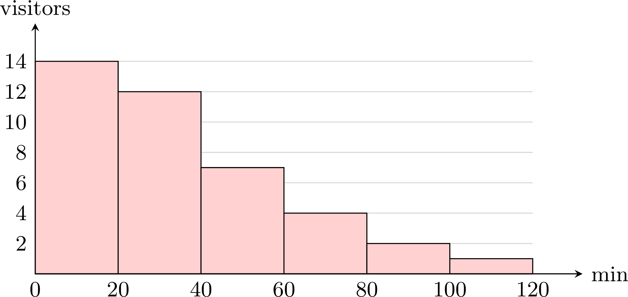

Where are most of the durations? On which side does the histogram stretch out?

Answer

Most visits are short: $14 + 12 = 26$ of the $40$ visits last less than $40$ minutes. Then the bars get shorter and shorter towards the long visits, up to the class from $100$ to $120$ minutes. The histogram stretches out on the right, in a long tail of rare, long visits: such a distribution is said to be skewed to the right.

Definition — Shape of a Distribution

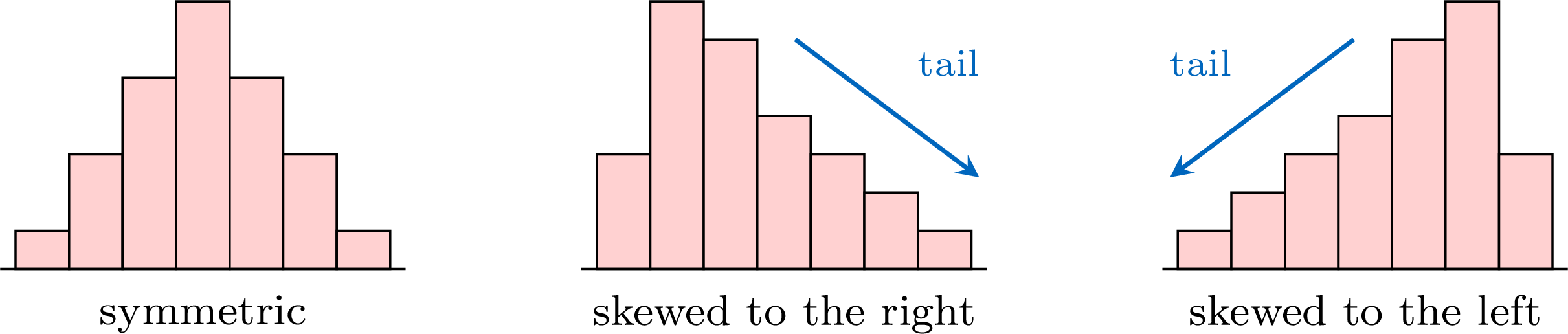
The distribution of a dataset is the way its values are spread along the axis, as a histogram or a bar chart shows it. Its shape is described by comparing its two sides.

The distribution is symmetric when its two sides, on either side of the middle, are roughly mirror images of each other.
It is skewed to the right (or positively skewed) when its graph has a long tail stretching towards the large values.
It is skewed to the left (or negatively skewed) when its long tail stretches towards the small values.

The side of the skew is the side of the tail, not the side of the peak.

Method — Reading the Shape on a Box Plot

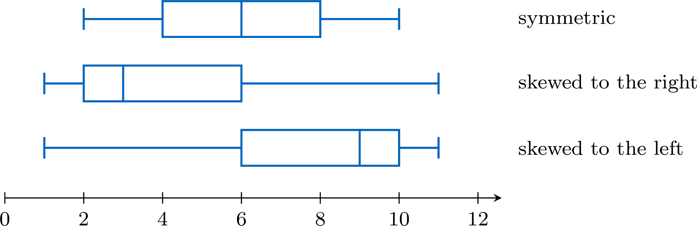
A box plot cuts the ordered data into four parts, each holding about a quarter of the values (when outliers are marked, they belong to the outer quarters, beyond the whiskers). Compare the two halves of the box (from $Q_1$ to the median, from the median to $Q_3$) and the two whiskers.

Symmetric: the median is near the middle of the box, and the two whiskers have about the same length.
Skewed to the right: the right half of the box and the right whisker are the longer ones — the median is closer to $Q_1$.
Skewed to the left: the left half of the box and the left whisker are the longer ones — the median is closer to $Q_3$.

A longer part does not hold more values: it holds the same quarter of the values, spread over a wider interval. When the box and the whiskers do not point the same way, the shape is not clear-cut: describe what each part shows. A box plot keeps only five numbers, so the shape it suggests is a clue, to be confirmed on a histogram when the data are available.

Example

The box plot shows the times, in minutes, that $40$ pupils took to solve a puzzle. Describe the shape of the distribution.

Answer

The five-number summary read on the plot is: minimum $2$, $Q_1 = 4$, median $5$, $Q_3 = 9$, maximum $16$. The lengths of the four parts are:

left whisker	left half of the box	right half of the box	right whisker
$4 - 2 = 2$	$5 - 4 = 1$	$9 - 5 = 4$	$16 - 9 = 7$

The right half of the box is four times as long as the left half, and the right whisker is longer than the left one: the distribution is skewed to the right. In context: the quarter of the pupils just below the median are packed between $4$ and $5$ minutes, whereas the slow times are spread out, up to $16$ minutes.

Method — Comparing the Mean and the Median

The mean uses the size of every value, whereas the median only depends on the value or values in the middle of the ordered list. A long tail therefore pulls the mean towards it, while the size of its values plays no part in the median.

Mean close to the median: consistent with a symmetric distribution.
Mean clearly greater than the median: the sign of a long tail on the right, that is of a distribution skewed to the right.
Mean clearly smaller than the median: the sign of a distribution skewed to the left.

This comparison is a clue, to be confirmed on a graph of the data (histogram or box plot).

Example

Eleven pupils noted how many minutes they spent on their phone one evening, in increasing order: $$15,\ 20,\ 25,\ 25,\ 30,\ 30,\ 35,\ 40,\ 45,\ 60,\ 115.$$

Compute the mean and the median.
What does their comparison suggest about the shape of the distribution?
The value $115$ is removed. Compute the new mean and the new median.

Answer

The mean is $$\begin{aligned}[t] \bar{x} &= \frac{15 + 20 + 25 + 25 + 30 + 30 + 35 + 40 + 45 + 60 + 115}{11} && \text{(definition of the mean)}\\ &= \frac{440}{11} && \text{(sum of the values)}\\ &= 40. \end{aligned}$$ There are $11$ ordered values: the median is the $6^{\text{th}}$ one, $30$.
The mean ($40$ minutes) is clearly greater than the median ($30$ minutes): this suggests a distribution skewed to the right. The list confirms it: the values climb slowly up to $45$, then jump to $60$ and $115$ — a long tail on the right. (With $Q_1 = 25$ and $Q_3 = 45$, the upper fence is $45 + 1.5 \times 20 = 75$: the value $115$ is even an outlier.)
Without $115$, the sum is $440 - 115 = 325$ for $10$ values, so the new mean is $\frac{325}{10} = 32.5$. The new median is the mean of the $5^{\text{th}}$ and $6^{\text{th}}$ of the $10$ values: $\frac{30 + 30}{2} = 30$. Removing one value of the tail lowered the mean by $7.5$ minutes and left the median unchanged.

Symmetric Does Not Mean Normal

Many measurements — the heights of adults, the masses of the apples of one orchard, the errors of a measuring instrument — have a bell-shaped distribution: a single peak in the middle, a symmetric shape, and frequencies that decrease steadily on both sides. The model of such data is called the normal distribution.
A normal distribution has a symmetric box plot, and data drawn from it usually give a nearly symmetric one. The converse is false: a symmetric box plot is consistent with a normal distribution, but it never proves it. The three datasets below all have a symmetric box plot; only the first one is bell-shaped.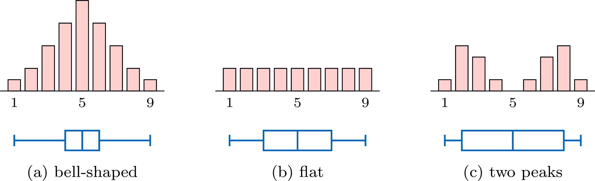

Their five-number summaries are $1, 4, 5, 6, 9$ for (a), $1, 3, 5, 7, 9$ for (b) and $1, 2, 5, 8, 9$ for (c): each box plot is symmetric about the median $5$. A box plot keeps only five numbers. To judge whether data may come from a normal distribution, look at the histogram as well: a single peak, in the middle, and frequencies that decrease on both sides.

Report an error

Skills to practice

Recognising the Shape of a Distribution
Justifying the Shape of a Distribution

II Comparing Data Sets and Judging Claims

II.1 Back-to-Back Stem-and-Leaf Plots and Parallel Box Plots

To compare two groups — two classes, two machines, two methods — their data are drawn on the same scale, one beside or above the other, so that the eye compares like with like. Two displays do this: the back-to-back stem-and-leaf plot, which keeps every value, and parallel box plots, which show the centre, the spread and the outliers of each group at a glance.

Report an error

Definition — Back-to-Back Stem-and-Leaf Plot

A back-to-back stem-and-leaf plot displays two data sets that share the same stems. The stems are written once, in a middle column; the leaves of one data set are written to the right, in increasing order away from the stem, and those of the other data set to the left, also in increasing order away from the stem — so they are read from right to left. A key explains both sides.

Example

The pulse rates at rest, in beats per minute, of $15$ pupils who do sport regularly and of $15$ pupils who do not are shown in the back-to-back stem-and-leaf plot.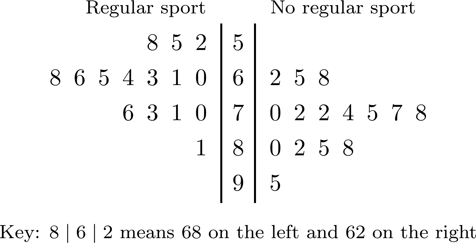

Find the median and the range of each group, then compare the two groups.

Answer

On the left, the leaves are read from the stem outwards: the row $6$ of the pupils who do sport stands for $60$, $61$, $63$, $64$, $65$, $66$, $68$.

Regular sport: with $15$ values, the median is the $8^{\text{th}}$. The row $5$ holds $3$ values, so the $8^{\text{th}}$ value is the $5^{\text{th}}$ of the row $6$: the median is $65$. The range is $81 - 52 = 29$.
No regular sport: the row $6$ holds $3$ values, so the $8^{\text{th}}$ value is the $5^{\text{th}}$ of the row $7$: the median is $75$. The range is $95 - 62 = 33$.

The leaves of the pupils who do sport lie about one row lower in value than those of the other pupils: their median is $10$ beats per minute lower, $65$ against $75$. The two ranges are close, $29$ and $33$: the two groups are about as spread out. For these pupils, those who do sport regularly have a lower pulse at rest.

Definition — Parallel Box Plots

Parallel box plots (or side-by-side box plots) are the box plots of two or more data sets, drawn one under the other above the same scale, each with the name of its data set. Their medians, their boxes and their whiskers can then be compared directly.

Method — Comparing Two Data Sets with Parallel Box Plots

Draw the two box plots above one scale, after testing each data set for outliers; the outliers are marked with crosses and the whiskers stop at the most extreme values that are not outliers.
Compare the centres: which median is higher, and by how much.
Compare the spreads: the interquartile ranges, the lengths of the boxes, and the ranges. The range depends on the two extreme values, so a single outlier can make it large; the interquartile range depends on the central half of the values and is hardly affected by one outlier: it is the better guide.
Note the outliers and the shapes of the two distributions.
Conclude in the context, naming each measure with its value and its data set.

When the two boxes hardly overlap, most values of one set are larger than most values of the other: the difference is clear. When they overlap a lot, the two sets have many values in the same range, and the comparison rests on the medians and the spreads together.

Example

Two pizzerias of a town, Rapido and Presto, both promise “delivery in half an hour”. The delivery times, in minutes, of $15$ orders from each are, in increasing order: $$\begin{aligned}&\text{Rapido: } 18,\ 20,\ 21,\ 22,\ 23,\ 24,\ 25,\ 25,\ 26,\ 27,\ 28,\ 29,\ 30,\ 32,\ 48,\\ &\text{Presto: } 14,\ 16,\ 19,\ 22,\ 24,\ 26,\ 28,\ 30,\ 31,\ 33,\ 35,\ 37,\ 40,\ 42,\ 45.\end{aligned}$$

Give the five-number summary of each pizzeria, and test each data set for outliers.
Draw the parallel box plots.
Compare the two pizzerias.

Answer

With $N = 15$ values, the median is the $8^{\text{th}}$ value; each half holds $7$ values, and the quartiles, the medians of the two halves, are the $4^{\text{th}}$ and $12^{\text{th}}$ values (the convention of quartiles as values of the dataset gives the same values).
- Rapido: minimum $18$, $Q_1 = 22$, median $25$, $Q_3 = 29$, maximum $48$. $\text{IQR} = 29 - 22 = 7$ and $1.5 \times \text{IQR} = 10.5$, so the fences are $22 - 10.5 = 11.5$ and $29 + 10.5 = 39.5$: the delivery of $48$ minutes is an outlier.
- Presto: minimum $14$, $Q_1 = 22$, median $30$, $Q_3 = 37$, maximum $45$. $\text{IQR} = 37 - 22 = 15$ and $1.5 \times \text{IQR} = 22.5$, so the fences are $-0.5$ and $59.5$: no outlier.
The right whisker of Rapido stops at $32$, its largest time that is not an outlier, and $48$ is marked by a cross.
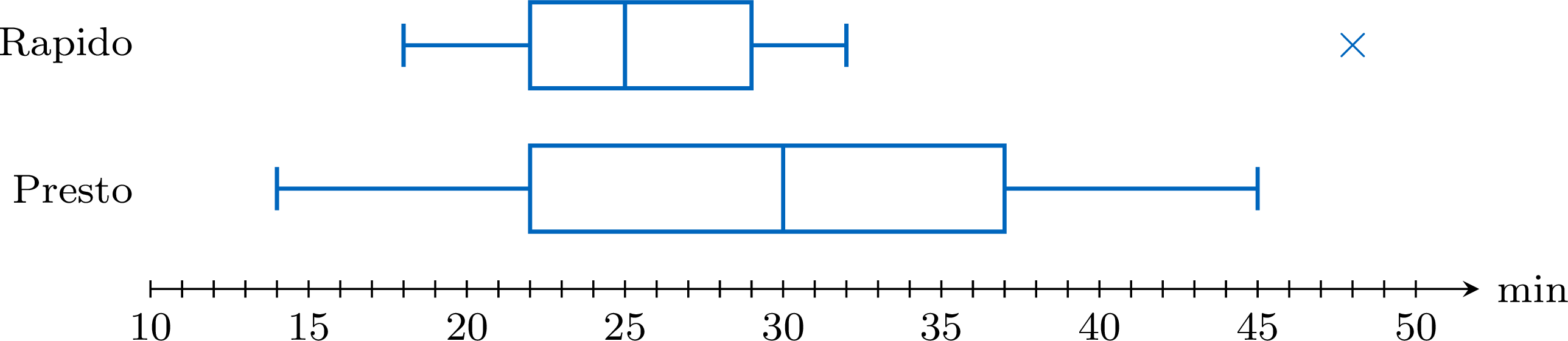
Centre: Rapido's median, $25$ minutes, is $5$ minutes below Presto's, $30$ minutes. Spread: Rapido's box is half as long, $\text{IQR} = 7$ minutes against $15$ minutes: its times are much more regular. The ranges, $30$ and $31$ minutes, are almost equal only because of Rapido's outlier. Outliers and shapes: one Rapido delivery took $48$ minutes, far from the others; apart from it, both box plots are roughly symmetric — the two halves of Rapido's box measure $3$ and $4$ minutes, those of Presto's $8$ and $7$ minutes, with whiskers of about the same length on each side. Conclusion: Rapido usually delivers faster and more regularly — $13$ of its $15$ deliveries took at most half an hour — but it had one very late delivery; Presto kept its promise of half an hour for only $8$ of its $15$ deliveries, as its median of $30$ minutes suggests.

How Far a Comparison Goes

A comparison describes the data collected. Rapido's $15$ deliveries were in general faster than Presto's — its median is lower, although some Presto deliveries were faster than some Rapido ones; the conclusion extends to all their deliveries only if the orders were chosen so that they represent them — at different hours and on different days, for example. With small samples, a small difference between the medians, inside boxes that overlap a lot, may come from the particular values that were collected: another sample could reverse it. A clear difference — boxes that hardly overlap — is more convincing.

Report an error

Skills to practice

Comparing Distributions
Reading Box Plots and Back-to-Back Plots
Interpreting and Comparing the Measures of Two Data Sets

II.2 Thinking Critically about Statistical Claims

Method — Thinking Critically About Statistical Claims

Whenever a claim based on statistics is met (e.g., in the news or an advertisement), it is evaluated critically. A good statistician considers two key points:

Question the Data Collection: All sample statistics contain potential error. Always ask:
- Was the sample representative of the population, or was it biased?
- Was the sample size large enough to be reliable?
- What is the potential for sampling error?
Avoid Overgeneralisation: Statistics describe group trends, not absolute truths about individuals. It is a common misuse of statistics to apply a group average to every member of that group.

Skills to practice

Thinking Critically about a Statistical Claim

III Going further

Skills to practice

Solving Problems with Box Plots
Conducting a Full Investigation
Investigating Patterns in Box Plots and Outliers
Quiz