International Baccalaureate · MYP 5

Statistics

⌚ ~27 min ▢ 3 blocks ✓ 12 exercises ➣ Prerequisites : Statistics: Sampling, Spread and Cumulative Frequency, Box Plots and Comparing Data Sets

I Reading and Using Percentiles

Definition — Cumulative-Frequency Curve (Ogive)

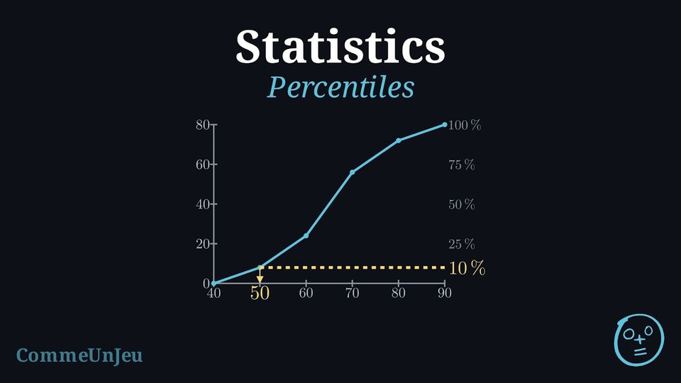
When data is grouped into classes, the running totals can be displayed graphically as the cumulative-frequency curve (or ogive). It is built by plotting each cumulative frequency against the upper boundary of its class and joining the points in order by straight segments, starting from the lower boundary of the first class at height $0$. The curve never goes down: it climbs from $0$ to the total $N$, and the number of values below any level can be estimated from it. In particular, the median is estimated by reading across from the height $\dfrac{N}{2}$ on the vertical axis to the curve, then down to the horizontal axis. In the same way, the lower quartile $Q_1$ and the upper quartile $Q_3$ are estimated by reading across from the heights $\dfrac{N}{4}$ and $\dfrac{3N}{4}$, which gives an estimate of the interquartile range $Q_3 - Q_1$.

Definition — Percentile

Let $k$ be a whole number from $1$ to $99$. A $k$-th percentile $P_k$ of a dataset is a value such that at least $k\pourcent$ of the values are less than or equal to $P_k$, and at least $(100 - k)\pourcent$ are greater than or equal to $P_k$: roughly, $k\pourcent$ of the data are less than or equal to $P_k$. For raw data several values may fit, and a convention chooses one, as for the quartiles. For data grouped in classes, $P_k$ is estimated on the cumulative frequency graph: it is the value at which the cumulative frequency reaches $k\pourcent$ of the total.
On a cumulative frequency graph, the quartiles are read as the percentiles of orders $25$, $50$ and $75$: $Q_1 = P_{25}$, the median is $P_{50}$ and $Q_3 = P_{75}$. For raw data, the quartiles taken as values of the dataset are percentiles in this sense, whereas the medians of the two halves can differ slightly from them. The percentiles $P_{10}$ and $P_{90}$ are also called the first and the ninth deciles.

Method — Reading Percentiles on a Cumulative Frequency Graph

On the cumulative frequency graph of a dataset of $N$ values:

Compute the height $\dfrac{k}{100} \times N$, or read $k\pourcent$ directly on a percentage scale.
Read across from this height on the vertical axis to the graph.
Read down to the horizontal axis: the value read is $P_k$.

Conversely, to find how many values lie below a value $x$, read up from $x$ to the graph, then across to the vertical axis: the cumulative frequency $c$ read means that about $c$ values, that is about $\dfrac{c}{N}$ of the data, are less than $x$, and about $N - c$ are greater than or equal to $x$. At a class boundary the count is exact; inside a class the polygon assumes the values are spread evenly, so the reading is an estimate, which can be computed by proportion, as for the median.

Example

The times of the $80$ runners of a $10$ km race are grouped in classes of $10$ minutes.

Time (min)	$[40, 50)$	$[50, 60)$	$[60, 70)$	$[70, 80)$	$[80, 90)$
Runners	$8$	$16$	$32$	$16$	$8$

Draw the cumulative frequency polygon, then use it to answer the following questions.

Estimate the quartiles and the interquartile range of the times.
The fastest $10\pourcent$ of the runners receive a medal. Which time did they beat?
What percentage of the runners finished in less than $70$ minutes? How many runners took more than $75$ minutes?

Answer

The cumulative frequencies, taken at the upper bounds $50, 60, 70, 80, 90$, are $8, 24, 56, 72, 80$; the polygon starts at $(40, 0)$. The right-hand scale gives the percentages of the $80$ runners.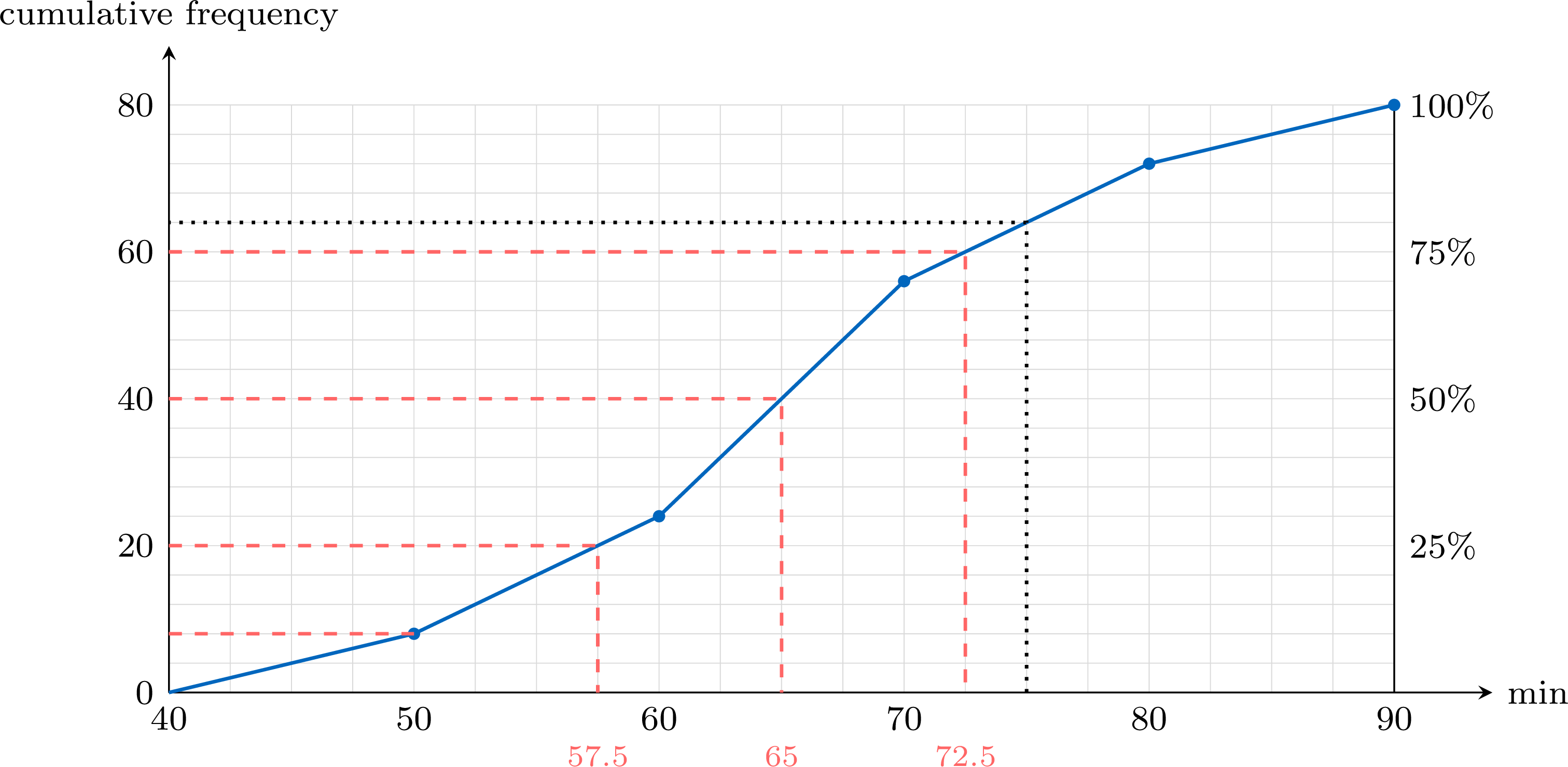

$Q_1 = P_{25}$ is read at the height $\frac{25}{100} \times 80 = 20$, the median at $40$ and $Q_3$ at $60$. The reading gives the estimates $Q_1 \approx 57.5$, median $\approx 65$ and $Q_3 \approx 72.5$ minutes. On the polygon each reading can be computed by proportion; for $Q_1$, the height $20$ lies in the class $[50, 60)$, between the cumulative frequencies $8$ and $24$: $$Q_1 \approx 50 + \frac{20 - 8}{24 - 8} \times 10 = 50 + 7.5 = 57.5.$$ The interquartile range is about $\text{IQR} = 72.5 - 57.5 = 15$ minutes.
The fastest runners are those with the smallest times: the fastest $10\pourcent$ are below $P_{10}$. The height $\frac{10}{100} \times 80 = 8$ is reached at $50$ minutes, a class boundary: exactly $8$ runners, the medal winners, finished in less than $50$ minutes.
Up from $70$ minutes, a class boundary, the cumulative frequency is $56$: $\frac{56}{80} = 70\pourcent$ of the runners finished in less than $70$ minutes. Up from $75$ minutes (dotted line), the polygon gives $64$: an estimated $80 - 64 = 16$ runners took more than $75$ minutes — an estimate, since $75$ lies inside the class $[70, 80)$.

A Percentile Is Not a Percentage of the Marks

Being at the $90$th percentile of a test means that about $90\pourcent$ of the candidates scored at most the same mark — not that the mark is $90\pourcent$ of the maximum. On a hard test, a mark of $12$ out of $20$ can be the $90$th percentile; on an easy one, $17$ out of $20$ can be the median. And when the best results are the smallest values, as for times, the best $10\pourcent$ lie below $P_{10}$, not above $P_{90}$.

Report an error

Skills to practice

Reading Percentiles on a Cumulative Frequency Graph
Interpreting and Using Percentiles

II Going further

Skills to practice

Investigating Patterns in Percentiles

Time (min)	\([40, 50)\)	\([50, 60)\)	\([60, 70)\)	\([70, 80)\)	\([80, 90)\)
Runners	\(8\)	\(16\)	\(32\)	\(16\)	\(8\)