International Baccalaureate · MYP 5 Extended

Statistics

⌚ ~98 min ▢ 10 blocks ✓ 42 exercises ➣ Prerequisites : Statistics: Sampling, Spread and Cumulative Frequency, Box Plots and Comparing Data Sets

I Reading and Using Percentiles

Definition — Cumulative-Frequency Curve (Ogive)

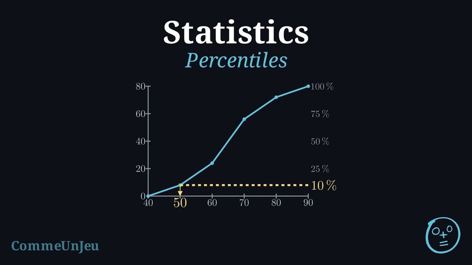
When data is grouped into classes, the running totals can be displayed graphically as the cumulative-frequency curve (or ogive). It is built by plotting each cumulative frequency against the upper boundary of its class and joining the points in order by straight segments, starting from the lower boundary of the first class at height $0$. The curve never goes down: it climbs from $0$ to the total $N$, and the number of values below any level can be estimated from it. In particular, the median is estimated by reading across from the height $\dfrac{N}{2}$ on the vertical axis to the curve, then down to the horizontal axis. In the same way, the lower quartile $Q_1$ and the upper quartile $Q_3$ are estimated by reading across from the heights $\dfrac{N}{4}$ and $\dfrac{3N}{4}$, which gives an estimate of the interquartile range $Q_3 - Q_1$.

Definition — Percentile

Let $k$ be a whole number from $1$ to $99$. A $k$-th percentile $P_k$ of a dataset is a value such that at least $k\pourcent$ of the values are less than or equal to $P_k$, and at least $(100 - k)\pourcent$ are greater than or equal to $P_k$: roughly, $k\pourcent$ of the data are less than or equal to $P_k$. For raw data several values may fit, and a convention chooses one, as for the quartiles. For data grouped in classes, $P_k$ is estimated on the cumulative frequency graph: it is the value at which the cumulative frequency reaches $k\pourcent$ of the total.
On a cumulative frequency graph, the quartiles are read as the percentiles of orders $25$, $50$ and $75$: $Q_1 = P_{25}$, the median is $P_{50}$ and $Q_3 = P_{75}$. For raw data, the quartiles taken as values of the dataset are percentiles in this sense, whereas the medians of the two halves can differ slightly from them. The percentiles $P_{10}$ and $P_{90}$ are also called the first and the ninth deciles.

Method — Reading Percentiles on a Cumulative Frequency Graph

On the cumulative frequency graph of a dataset of $N$ values:

Compute the height $\dfrac{k}{100} \times N$, or read $k\pourcent$ directly on a percentage scale.
Read across from this height on the vertical axis to the graph.
Read down to the horizontal axis: the value read is $P_k$.

Conversely, to find how many values lie below a value $x$, read up from $x$ to the graph, then across to the vertical axis: the cumulative frequency $c$ read means that about $c$ values, that is about $\dfrac{c}{N}$ of the data, are less than $x$, and about $N - c$ are greater than or equal to $x$. At a class boundary the count is exact; inside a class the polygon assumes the values are spread evenly, so the reading is an estimate, which can be computed by proportion, as for the median.

Example

The times of the $80$ runners of a $10$ km race are grouped in classes of $10$ minutes.

Time (min)	$[40, 50)$	$[50, 60)$	$[60, 70)$	$[70, 80)$	$[80, 90)$
Runners	$8$	$16$	$32$	$16$	$8$

Draw the cumulative frequency polygon, then use it to answer the following questions.

Estimate the quartiles and the interquartile range of the times.
The fastest $10\pourcent$ of the runners receive a medal. Which time did they beat?
What percentage of the runners finished in less than $70$ minutes? How many runners took more than $75$ minutes?

Answer

The cumulative frequencies, taken at the upper bounds $50, 60, 70, 80, 90$, are $8, 24, 56, 72, 80$; the polygon starts at $(40, 0)$. The right-hand scale gives the percentages of the $80$ runners.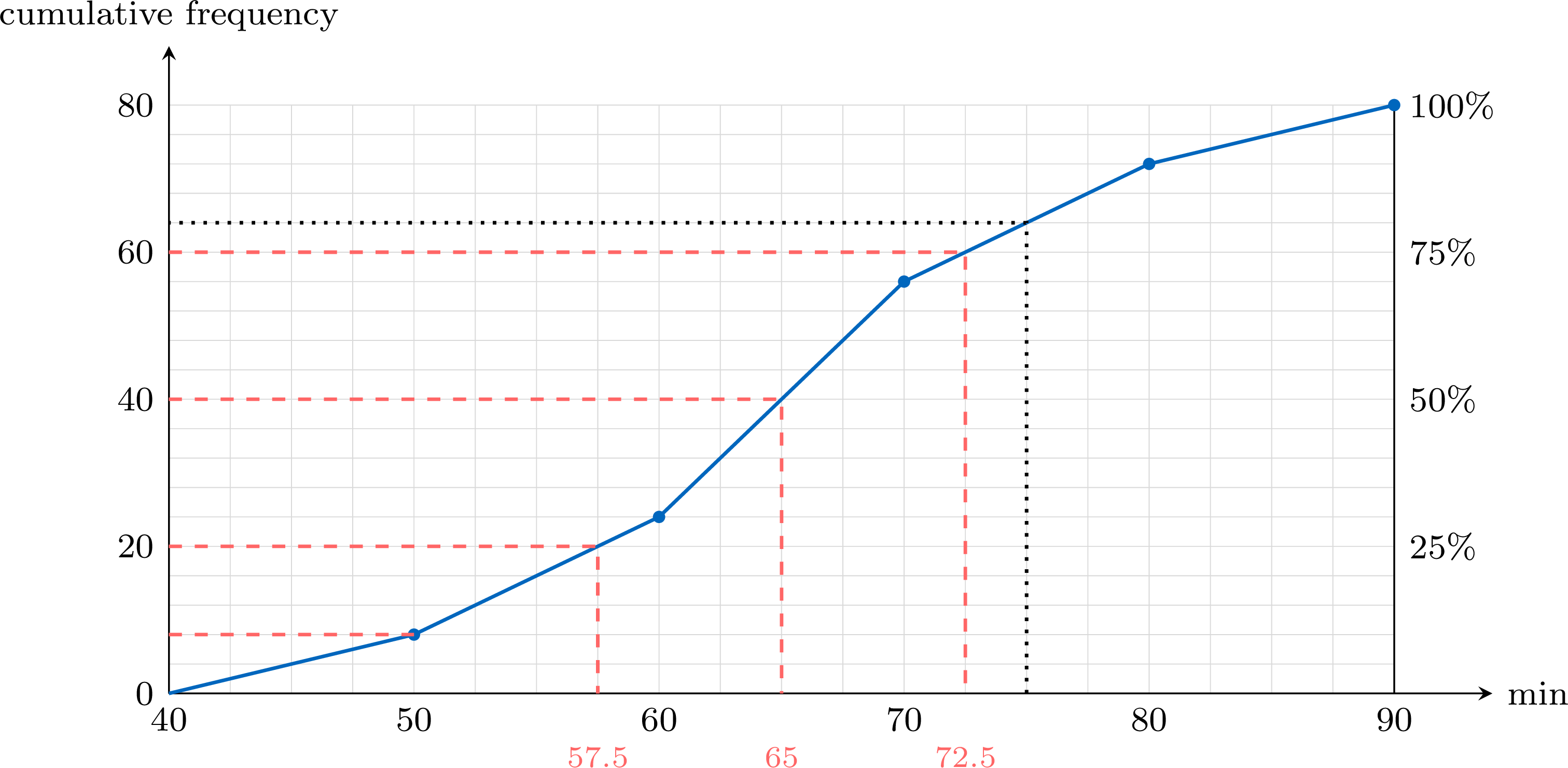

$Q_1 = P_{25}$ is read at the height $\frac{25}{100} \times 80 = 20$, the median at $40$ and $Q_3$ at $60$. The reading gives the estimates $Q_1 \approx 57.5$, median $\approx 65$ and $Q_3 \approx 72.5$ minutes. On the polygon each reading can be computed by proportion; for $Q_1$, the height $20$ lies in the class $[50, 60)$, between the cumulative frequencies $8$ and $24$: $$Q_1 \approx 50 + \frac{20 - 8}{24 - 8} \times 10 = 50 + 7.5 = 57.5.$$ The interquartile range is about $\text{IQR} = 72.5 - 57.5 = 15$ minutes.
The fastest runners are those with the smallest times: the fastest $10\pourcent$ are below $P_{10}$. The height $\frac{10}{100} \times 80 = 8$ is reached at $50$ minutes, a class boundary: exactly $8$ runners, the medal winners, finished in less than $50$ minutes.
Up from $70$ minutes, a class boundary, the cumulative frequency is $56$: $\frac{56}{80} = 70\pourcent$ of the runners finished in less than $70$ minutes. Up from $75$ minutes (dotted line), the polygon gives $64$: an estimated $80 - 64 = 16$ runners took more than $75$ minutes — an estimate, since $75$ lies inside the class $[70, 80)$.

A Percentile Is Not a Percentage of the Marks

Being at the $90$th percentile of a test means that about $90\pourcent$ of the candidates scored at most the same mark — not that the mark is $90\pourcent$ of the maximum. On a hard test, a mark of $12$ out of $20$ can be the $90$th percentile; on an easy one, $17$ out of $20$ can be the median. And when the best results are the smallest values, as for times, the best $10\pourcent$ lie below $P_{10}$, not above $P_{90}$.

Report an error

Skills to practice

Reading Percentiles on a Cumulative Frequency Graph
Interpreting and Using Percentiles

II Measuring Spread with the Standard Deviation

The standard deviation measures spread using every value of the data set. It measures the typical distance of the values from the mean (more precisely, the root-mean-square distance). A small standard deviation means the values are clustered closely around the mean, while a large standard deviation means they are spread out.

Report an error

Definition — Standard Deviation

The standard deviation ($\sigma$) is found by taking the square root of the average of the squared differences from the mean.$$\sigma = \sqrt{\frac{\sum_{i=1}^{n}(x_i - \bar{x})^2}{n}}$$ where $\bar{x}$ is the mean and $n$ is the number of data points. This is the population (descriptive) standard deviation; when a sample is used to estimate a population, a variant divides by $n-1$ instead of $n$. The symbol $\sum$ means “sum over all the values”.

Example

Find the standard deviation for the data: $$2, 4, 4, 4, 5, 5, 7, 9$$

Answer

Find the mean ($\bar{x}$): $$ \bar{x} = \frac{2 + 4 + 4 + 4 + 5 + 5 + 7 + 9}{8} = \frac{40}{8} = 5 $$
Calculate the squared differences from the mean: $(2-5)^2 = 9$, $(4-5)^2 = 1$, $(4-5)^2 = 1$, $(4-5)^2 = 1$, $(5-5)^2 = 0$, $(5-5)^2 = 0$, $(7-5)^2 = 4$, $(9-5)^2 = 16$.
Find the average of the squared differences (the variance): $$ \frac{9 + 1 + 1 + 1 + 0 + 0 + 4 + 16}{8} = \frac{32}{8} = 4 $$
Take the square root to find the standard deviation ($\sigma$): $$ \sigma = \sqrt{4} = 2 $$

The standard deviation is 2.

Skills to practice

Calculating a Standard Deviation

III Finding the Variance and Standard Deviation from a Frequency Table

Definition — Variance and Standard Deviation

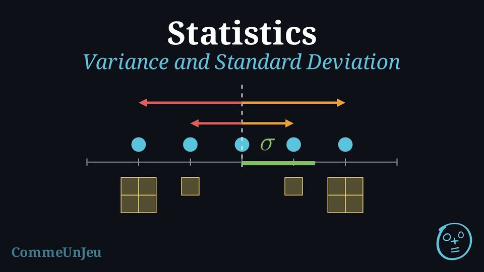
The variance $V$ of a data set measures the average of the squared distances of the values from the mean $\bar{x}$. When the values $x_i$ have frequencies $n_i$ (with $N = \sum n_i$): $$ V = \frac{1}{N}\sum_{i=1}^{k} n_i (x_i - \bar{x})^2 . $$ The standard deviation $\sigma$ is the square root of the variance: $$ \sigma = \sqrt{V} = \sqrt{\frac{1}{N}\sum_{i=1}^{k} n_i (x_i - \bar{x})^2} . $$ The variance is expressed in the squared unit of the data, whereas the standard deviation is back in the original unit, which makes it the natural measure of typical distance to the mean. This is the population (descriptive) variance, with denominator $N$.

Example

During $10$ matches, a player scored the numbers of goals given in the frequency table below. Compute the variance $V$ and the standard deviation $\sigma$ of the number of goals.

Goals $x_i$	0	1	2	3	Total
Frequency $n_i$	3	4	2	1	10

Answer

Step 1 — Mean. With $N = 3+4+2+1 = 10$ and $\sum n_i x_i = 0\cdot 3 + 1\cdot 4 + 2\cdot 2 + 3\cdot 1 = 11$: $$ \bar{x} = \frac{11}{10} = 1.1 . $$ Step 2 — Squared deviations weighted by frequency.

$x_i$	$n_i$	$x_i-\bar{x}$	$(x_i-\bar{x})^2$	$n_i(x_i-\bar{x})^2$
0	3	$-1.1$	$1.21$	$3.63$
1	4	$-0.1$	$0.01$	$0.04$
2	2	$0.9$	$0.81$	$1.62$
3	1	$1.9$	$3.61$	$3.61$
Total	10			8.90

Step 3 — Variance, then standard deviation. $$ \begin{aligned} V &= \frac{1}{N}\sum n_i (x_i-\bar{x})^2 &&\text{(definition)} \\ &= \frac{8.90}{10} &&\text{(substitute)} \\ &= 0.89 ; &&\text{(divide)} \\ \sigma &= \sqrt{V} = \sqrt{0.89} &&\text{(square root)} \\ &\approx 0.94 . &&\text{(evaluate)} \end{aligned} $$ The variance is $0.89$ goal$^2$ and the standard deviation is about $0.94$ goal.

Skills to practice

Calculating a Variance and a Standard Deviation

IV Comparing with the Mean and the Standard Deviation

Method — Choosing the Measures to Compare

To compare two datasets, pair a measure of centre with its measure of spread:

the mean $\bar{x}$ goes with the standard deviation $\sigma$ — they use every value, but extreme values pull them;
the median goes with the interquartile range — they are read off positions in the ordered list, so one extreme value barely moves them.

When the data contain extreme values, prefer the pair median–IQR; otherwise prefer the pair mean–$\sigma$, which takes every value into account. Conclude with a sentence naming both measures.

Example

Two sellers each worked $9$ days. Their daily sales are: $$\text{Seller A: } 4,\ 5,\ 5,\ 6,\ 6,\ 7,\ 7,\ 8,\ 42 \qquad \text{Seller B: } 8,\ 9,\ 9,\ 10,\ 10,\ 10,\ 11,\ 11,\ 12.$$ Both means equal $10$. Compare the two sellers with the appropriate pair of indicators.

Answer

Seller A's list holds the extreme value $42$: the means are pulled, so we choose the pair median–IQR. With $N = 9$ values, the median is the $5^{\text{th}}$ value, and the quartiles are the medians of the two halves (the median left out).

Seller A: median $= 6$; the lower half $4, 5, 5, 6$ gives $Q_1 = 5$ and the upper half $7, 7, 8, 42$ gives $Q_3 = 7.5$, so $\text{IQR} = 7.5 - 5 = 2.5$.
Seller B: median $= 10$; the lower half $8, 9, 9, 10$ gives $Q_1 = 9$ and the upper half $10, 11, 11, 12$ gives $Q_3 = 11$, so $\text{IQR} = 11 - 9 = 2$.

(With the values-of-the-dataset convention, $\frac{N}{4} = 2.25$ and $\frac{3N}{4} = 6.75$: the quartiles are the $3^{\text{rd}}$ and $7^{\text{th}}$ values, and both interquartile ranges equal $2$.)
Similar spreads (IQR $2.5$ and $2$), but B's median ($10$) is well above A's ($6$): on a typical day B sells more — A's mean of $10$ only comes from the exceptional day at $42$.

The standard deviation is above all a comparison instrument. Two data sets can share the same mean yet differ greatly in how the values are scattered around it: the set with the smaller standard deviation is the more consistent (regular) one. For example, a striker who scores $\{2,3,4,5,6\}$ goals across five matches and one who scores $\{3,4,4,4,5\}$ both average $4$ goals; their variances are $2$ and $0.4$ respectively, so the second striker is far more consistent — the same average hides very different regularity.

Report an error

Skills to practice

Comparing Data Sets with the Mean and the Standard Deviation

V Modelling with the Normal Curve

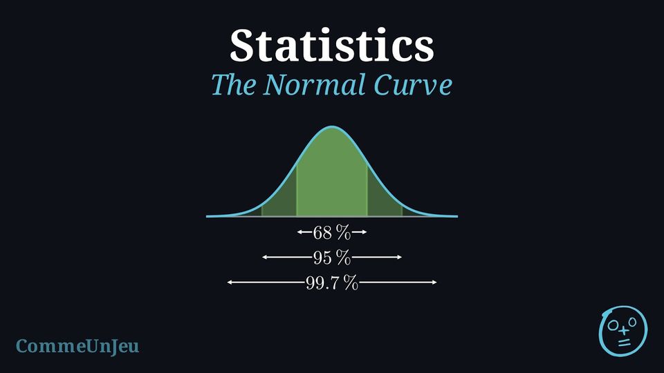
Many measurements — the heights of the adult women of a country, the masses of the eggs of a farm, the errors of a measuring instrument — give a histogram with a single peak in the middle, a symmetric shape, and frequencies that decrease on both sides. With many values, the classes can be made narrower and the outline of the histogram becomes a smooth curve. For many measurements of this kind, that curve is very close to a normal curve: one particular bell-shaped curve, set by the mean and the standard deviation of the data. The figure shows the histogram of the heights, in centimetres, of $1\,000$ adult women, with the normal curve that models it.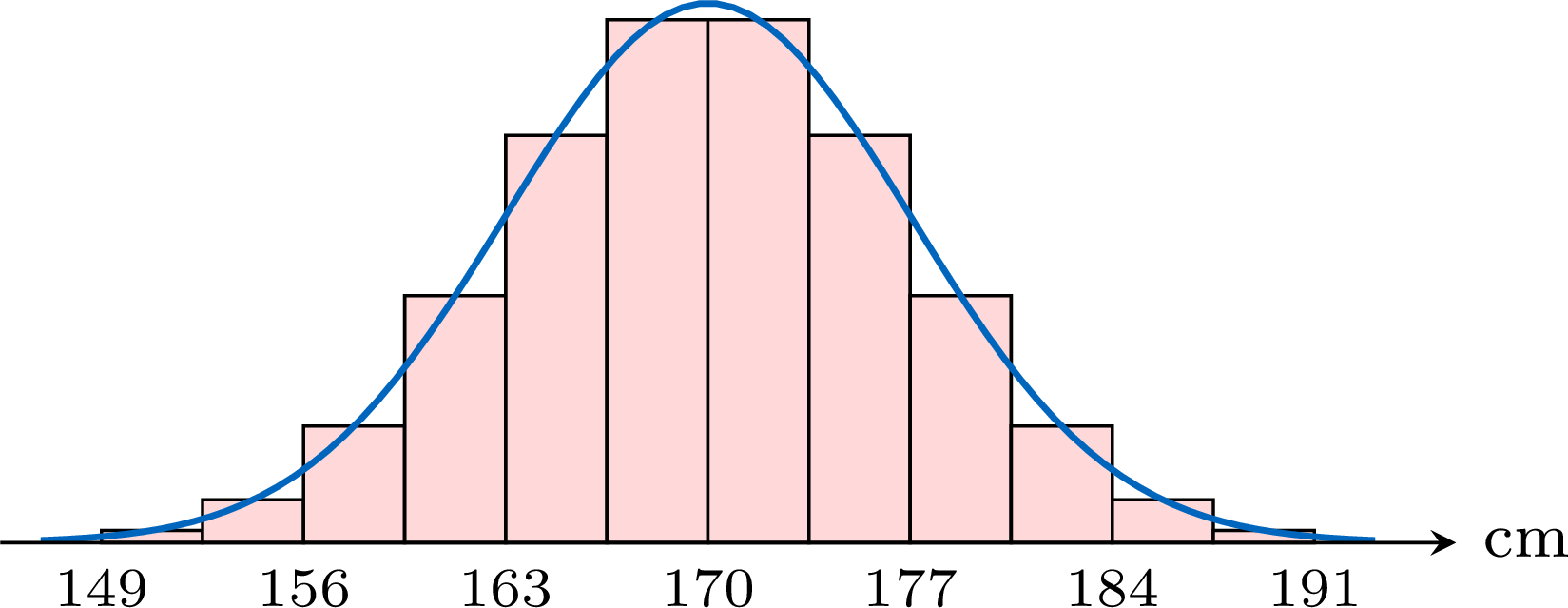

The curve describes the whole distribution at once: where the values are centred, how spread out they are, and which proportion of them lies in any interval.

Report an error

Definition — Normal Distribution

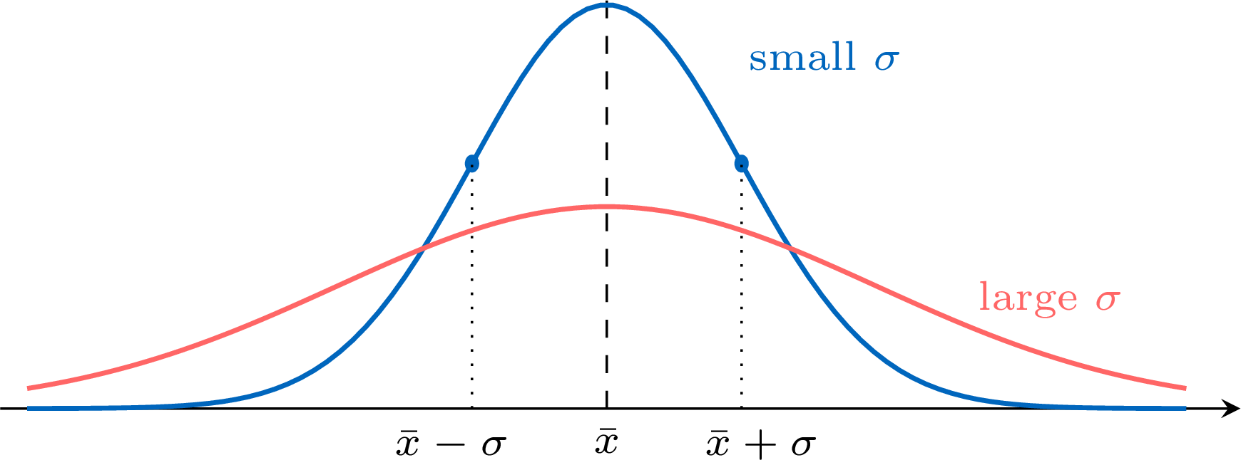
A normal curve is one particular bell-shaped curve, entirely set by two numbers: a mean $\bar{x}$ and a standard deviation $\sigma$ (its equation is not needed here). A data set is normally distributed, or follows a normal distribution, when its histogram, for many values and narrow classes, is very close to the normal curve with the same mean and the same standard deviation. Every normal curve

has a single peak, above the mean $\bar{x}$;
is symmetric about the vertical line through $\bar{x}$, so that the mean, the median and the mode are equal (approximately, for real data);
decreases on both sides of the mean and comes closer and closer to the horizontal axis without reaching it: values far from the mean are rare, but not impossible.

The mean $\bar{x}$ sets the position of the curve and the standard deviation $\sigma$ sets its width: the larger $\sigma$, the wider and flatter the bell. On the curve, $\bar{x} - \sigma$ and $\bar{x} + \sigma$ are the two places where the curve changes the way it bends: between them it bends downwards, beyond them it bends upwards (the two dots on the narrow curve of the figure). The proportion of the values lying between two numbers is shown by the part of the region under the curve between them. Other bell-shaped curves also have a single peak, an axis of symmetry and two tails: these properties describe a normal curve, they do not define it.

Proposition — The 68–95–99.7 Rule

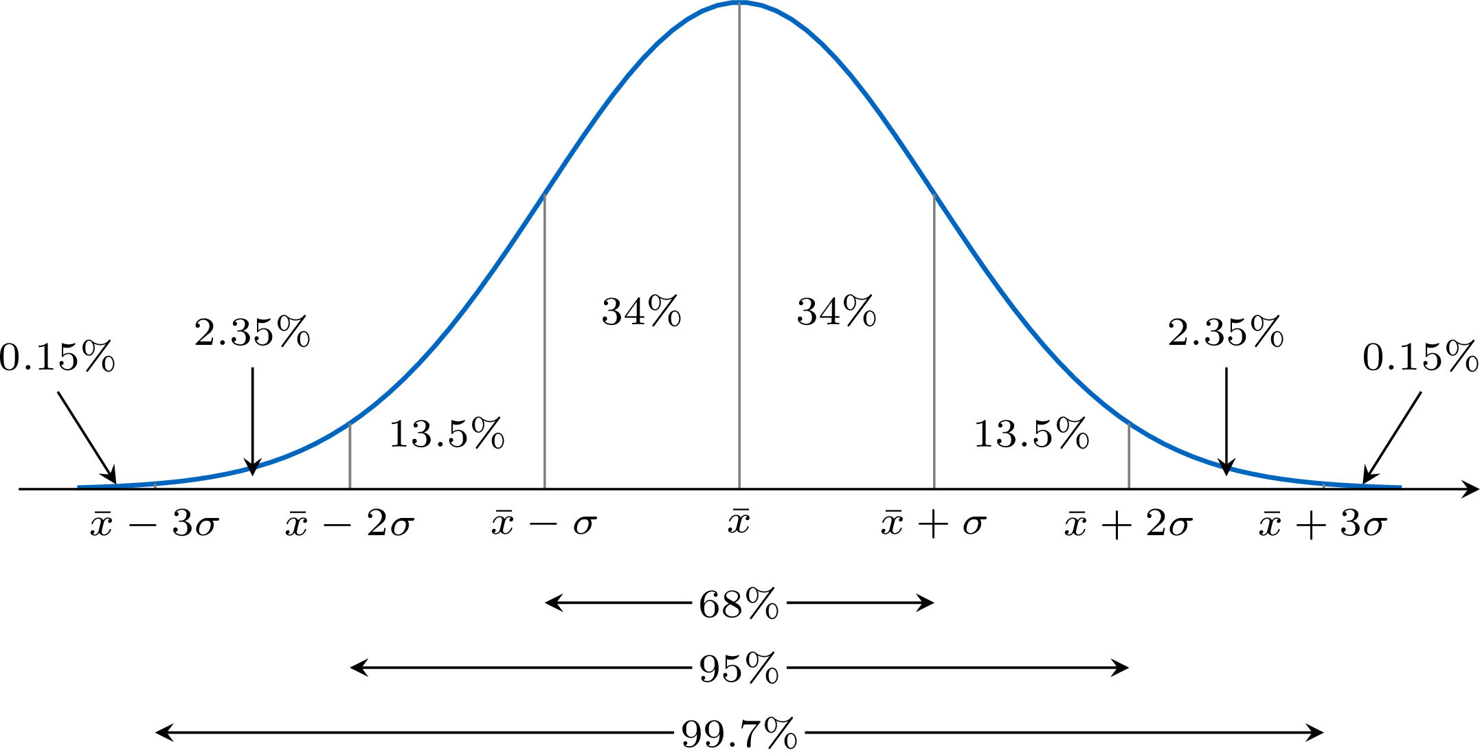
For a data set that is normally distributed with mean $\bar{x}$ and standard deviation $\sigma$:

about $68\pourcent$ of the values lie between $\bar{x} - \sigma$ and $\bar{x} + \sigma$;
about $95\pourcent$ of the values lie between $\bar{x} - 2\sigma$ and $\bar{x} + 2\sigma$;
about $99.7\pourcent$ of the values lie between $\bar{x} - 3\sigma$ and $\bar{x} + 3\sigma$.

By symmetry, each proportion splits into two equal halves on either side of the mean, which gives the proportion of each band:

These percentages are properties of the normal curve; for real data they give approximate proportions.

When the Rule Applies

The rule holds for data that are normally distributed, and only approximately, since real data are at best close to normal: the larger the data set, the closer the proportions usually are to $68\pourcent$, $95\pourcent$ and $99.7\pourcent$. It does not hold for every data set, not even for every symmetric one. The ten digits $0, 1, \ldots, 9$, each taken once, have the mean $$\bar{x} = \frac{0 + 1 + \cdots + 9}{10} = 4.5$$ and the standard deviation $\sigma = \sqrt{8.25} \approx 2.87$. The interval from $\bar{x} - \sigma \approx 1.63$ to $\bar{x} + \sigma \approx 7.37$ contains the six digits $2, 3, 4, 5, 6, 7$, that is $60\pourcent$ of the values, not $68\pourcent$: the distribution is symmetric but flat, not bell-shaped. Before using the rule, check on a histogram that the data are bell-shaped; even then, a bell shape makes the normal model reasonable, it does not prove it. For normal data, only about $0.3\pourcent$ of the values lie more than $3\sigma$ away from the mean, about $3$ values in $1\,000$: such a value is very unusual.

Report an error

Method — Using the 68–95–99.7 Rule

For data that are normally distributed with mean $\bar{x}$ and standard deviation $\sigma$:

Sketch the curve: draw a bell centred on $\bar{x}$ and mark $\bar{x} \pm \sigma$, $\bar{x} \pm 2\sigma$ and $\bar{x} \pm 3\sigma$ on its axis, with their values.
Use the bands: $50\pourcent$ of the values on each side of the mean; then, on each side, about $34\pourcent$ between the mean and $1\sigma$, about $\frac{95 - 68}{2} = 13.5\pourcent$ between $1\sigma$ and $2\sigma$, about $\frac{99.7 - 95}{2} = 2.35\pourcent$ between $2\sigma$ and $3\sigma$, and about $\frac{100 - 99.7}{2} = 0.15\pourcent$ beyond $3\sigma$. These band values come from the rounded percentages of the rule: they are approximate too.
Add the bands that make up the interval asked for (a half of the curve counts $50\pourcent$).
Convert to a number of values when asked: number $\approx$ proportion $\times$ total number of values, rounded to a whole number.

Conversely, a known proportion in a tail tells how many standard deviations a value is from the mean: $16\pourcent$ above a value places it at $\bar{x} + \sigma$, $2.5\pourcent$ above it at $\bar{x} + 2\sigma$.

Example

The masses of the $400$ eggs laid on a farm one week are normally distributed with mean $60$ g and standard deviation $4$ g.

Between which two masses do about $95\pourcent$ of the eggs lie?
What percentage of the eggs have a mass greater than $64$ g?
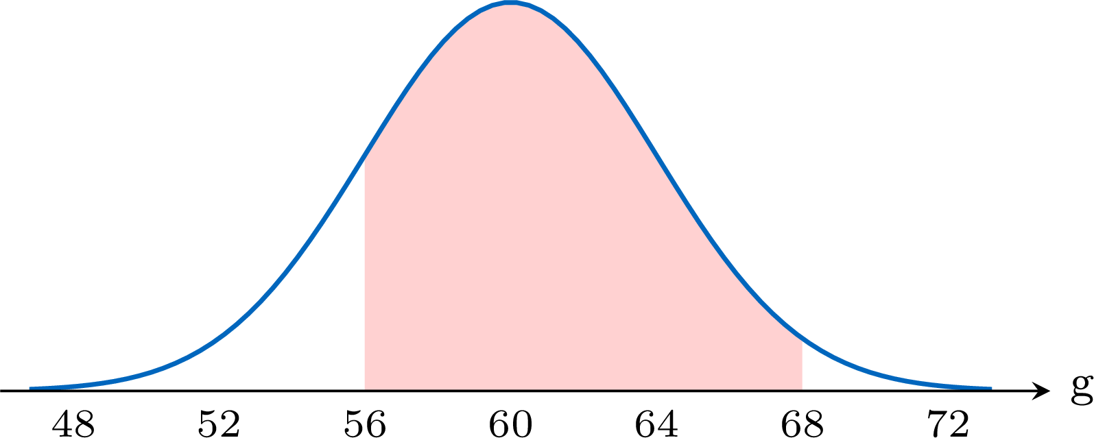
About how many eggs have a mass between $56$ g and $68$ g?

Answer

Here $\bar{x} = 60$ g and $\sigma = 4$ g, so the marks of the axis are $48$, $52$, $56$, $60$, $64$, $68$ and $72$ g.

About $95\pourcent$ of the values lie within $2\sigma$ of the mean: $$\bar{x} - 2\sigma = 60 - 2 \times 4 = 52 \qquad \text{and} \qquad \bar{x} + 2\sigma = 60 + 2 \times 4 = 68.$$ About $95\pourcent$ of the eggs have a mass between $52$ g and $68$ g.
$64 = 60 + 4 = \bar{x} + \sigma$. Above $\bar{x} + \sigma$ lie the three outer bands on the right: $$\begin{aligned}[t] \text{percentage above } 64 \text{ g} &= 13.5 + 2.35 + 0.15 &&\text{(bands beyond } \bar{x} + \sigma\text{)}\\ &= 16\pourcent. \end{aligned}$$ (Or: $50\pourcent$ above the mean, minus the $34\pourcent$ between $60$ and $64$.) About $16\pourcent$ of the eggs have a mass greater than $64$ g.
$56 = \bar{x} - \sigma$ and $68 = \bar{x} + 2\sigma$: $$\begin{aligned}[t] \text{proportion between } 56 \text{ and } 68 \text{ g} &= 34 + 34 + 13.5 &&\text{(bands from } \bar{x} - \sigma \text{ to } \bar{x} + 2\sigma\text{)}\\ &= 81.5\pourcent,\\ \text{number of eggs} &\approx 0.815 \times 400 &&\text{(proportion} \times \text{total)}\\ &= 326. \end{aligned}$$ About $326$ eggs have a mass between $56$ g and $68$ g.

Example

A machine fills bottles of water. The volumes are normally distributed with mean $500$ mL, and about $2.5\pourcent$ of the bottles contain more than $506$ mL.

Estimate the standard deviation of the volumes.
Estimate the percentage of the bottles that contain less than $497$ mL.

Answer

The percentage above $\bar{x} + 2\sigma$ is $2.35 + 0.15 = 2.5\pourcent$. So $506$ mL is at $\bar{x} + 2\sigma$: $$\begin{aligned}[t] 500 + 2\sigma &= 506 &&(\bar{x} + 2\sigma = 506)\\ 2\sigma &= 6\\ \sigma &= 3. \end{aligned}$$ The standard deviation is about $3$ mL.
$497 = 500 - 3 = \bar{x} - \sigma$. Below $\bar{x} - \sigma$ lie the three outer bands on the left: $$\begin{aligned}[t] \text{percentage below } 497 \text{ mL} &= 13.5 + 2.35 + 0.15 &&\text{(bands beyond } \bar{x} - \sigma\text{)}\\ &= 16\pourcent. \end{aligned}$$ About $16\pourcent$ of the bottles contain less than $497$ mL.

Skills to practice

Recognising a Normal Distribution
Using the 68–95–99.7 Rule
Solving Problems with a Normal Distribution

VI Going further

Skills to practice

Conducting a Full Investigation
Investigating Patterns in Percentiles
Quiz

Time (min)	\([40, 50)\)	\([50, 60)\)	\([60, 70)\)	\([70, 80)\)	\([80, 90)\)
Runners	\(8\)	\(16\)	\(32\)	\(16\)	\(8\)

\(x_i\)	\(n_i\)	\(x_i-\bar{x}\)	\((x_i-\bar{x})^2\)	\(n_i(x_i-\bar{x})^2\)
0	3	\(-1.1\)	\(1.21\)	\(3.63\)
1	4	\(-0.1\)	\(0.01\)	\(0.04\)
2	2	\(0.9\)	\(0.81\)	\(1.62\)
3	1	\(1.9\)	\(3.61\)	\(3.61\)
Total	10			8.90