International Baccalaureate · DP 2: Applications and Interpretation SL

Direct and Inverse Variation

⌚ ~66 min ▢ 6 blocks ✓ 20 exercises ➣ Prerequisites : Quadratic Functions, Functions, Modelling, Direct and Inverse Proportion

I Determining a Variation Model

Definition — Proportion with a Power

Let $n$ be a positive whole number and $k$ a nonzero number.

$y$ is directly proportional to $x^n$ when $y = kx^n$ for every pair of matching values. We write $y \propto x^n$. For $n = 2$, $y$ is proportional to the square of $x$; for $n = 3$, to the cube of $x$.
$y$ is inversely proportional to $x^n$ when $y = \dfrac{k}{x^n}$ for every pair of matching values, with $x \neq 0$. We write $y \propto \dfrac{1}{x^n}$. For $n = 2$, this is the inverse-square law.

For $n = 1$, these are direct proportion and inverse proportion.

Proposition — Asymptotic Behaviour

For $k \neq 0$ and $n$ a positive integer, the graph of the inverse variation model $y = \dfrac{k}{x^n} = kx^{-n}$ (the form $ax^m$ with $m < 0$) has the $y$-axis, $x = 0$, as a vertical asymptote and the $x$-axis, $y = 0$, as a horizontal asymptote.

Method — Recognising the Law from a Table

For each column of the table (with $x \neq 0$):

compute $\dfrac{y}{x}$ and $xy$, then, if neither is constant, $\dfrac{y}{x^2}$ and $x^2y$, then $\dfrac{y}{x^3}$ and $x^3y$;
keep the calculation that gives the same number in every column: if $\dfrac{y}{x^n}$ is constant, $y \propto x^n$; if $x^ny$ is constant, $y \propto \dfrac{1}{x^n}$; that number is the constant $k$;
if no calculation is constant, the table shows none of the laws tested here ($n = 1$, $2$ or $3$) — one column that breaks the pattern is enough.

Two columns in which $x$ is doubled give a first guess (Remark “Telling the Laws Apart”), which the calculation then confirms.

Example

Each table comes from an experiment. Determine the variation model that each table follows.

The air resistance $R$, in newtons, on a cyclist riding at $v$ metres per second.

$v$ $2$ $4$ $6$ $8$

$R$ $1.2$ $4.8$ $10.8$ $19.2$

Then predict the air resistance at $10$ metres per second.
The time $T$, in hours, that $w$ workers need to paint a hall.

$w$ $2$ $3$ $4$ $6$

$T$ $18$ $12$ $9$ $6$

Answer

$R$ increases with $v$, so we test direct variation with a power of $v$: we compute $\frac{R}{v}$, then $\frac{R}{v^2}$, for every data point.

$v$ $2$ $4$ $6$ $8$

$\frac{R}{v}$ $0.6$ $1.2$ $1.8$ $2.4$

$\frac{R}{v^2}$ $0.3$ $0.3$ $0.3$ $0.3$

The ratio $\frac{R}{v}$ is not constant, so $R$ does not vary directly with $v$. The ratio $\frac{R}{v^2}$ is constant, equal to $0.3$: $R$ varies directly with the square of $v$, $R \propto v^2$, and $R = 0.3v^2$. Check with doubling: from $v = 2$ to $v = 4$, $R$ is multiplied by $\frac{4.8}{1.2} = 4 = 2^2$, as a square law predicts. At $v = 10$: $$R = 0.3 \times 10^2 = 30.$$ The model predicts an air resistance of $30$ newtons.
$T$ decreases when $w$ increases, so we test inverse variation: we compute the product $wT$ for every data point: $2 \times 18 = 36$, $3 \times 12 = 36$, $4 \times 9 = 36$, $6 \times 6 = 36$. The product is constant, so $T$ varies inversely with $w$: $T \propto \frac{1}{w}$ and $T = \frac{36}{w}$. The constant $36$ is the number of hours one worker alone would need, if the law held for one worker: $w = 1$ lies outside the data, so this reading is an extrapolation.

Skills to practice

Finding a Variation Model with a Power
Fitting a Variation Model to Measured Data

II Finding the Parameters of a Model

Recappreviously studied — click to reread

Method — Finding the Parameters of a Model from Data Points

When the form of a model is known but its parameters are not, data points give the parameters.

Choose the form of the model from the context or from the shape of the data, and count its unknown parameters.
Substitute each data point $(x, y)$ in the model: each point gives one equation whose unknowns are the parameters. When each parameter only multiplies a known expression in $x$ — a polynomial model, or a model such as $\frac{a}{x} + b$ — these equations are linear in the parameters, even when the model is not linear in $x$. A value read directly, such as the value at $x = 0$ of a polynomial model, gives a parameter at once and removes one unknown.
Solve the system with the linear system solver. Use as many data points as unknown parameters, so that the system has as many equations as unknowns, and check that the solver shows a unique solution. If it reports infinitely many, the points do not fix the parameters: replace one of them. If it reports no solution, no model of this form passes through all the points: reconsider the data or the form of the model.
Check the parameters with every data point, then write the model.
State the domain on which the model is used and, when another data point is available, test the model on it.

Example

A workshop makes wooden chairs. The cost per chair, $C$ dollars, when $n$ chairs are made in a week, is modelled by $C = \dfrac{a}{n} + b$. When $100$ chairs are made, the cost is $\dollar 70$ per chair; when $400$ chairs are made, it is $\dollar 40$ per chair.

Use technology to find $a$ and $b$, then interpret them.
Predict the cost per chair when $1\,000$ chairs are made in a week.

Answer

The model is not linear in $n$, but it is linear in $a$ and $b$. Each data point gives one equation:
- $(100, 70)$: $\dfrac{a}{100} + b = 70$, that is $0.01a + b = 70$;
- $(400, 40)$: $\dfrac{a}{400} + b = 40$, that is $0.0025a + b = 40$.
The linear system solver, with two unknowns and the rows $0.01$, $1$, $70$ and $0.0025$, $1$, $40$, displays $a = 4\,000$ and $b = 30$. Check: $\frac{4\,000}{100} + 30 = 70$ and $\frac{4\,000}{400} + 30 = 40$. The model is $C = \dfrac{4\,000}{n} + 30$.
Interpretation: $\frac{a}{n}$ shares $a$ between the $n$ chairs, so $a = 4\,000$ is the fixed weekly cost, in dollars, whatever the number of chairs (rent, machines); $b = 30$ is the cost, in dollars, of the wood and the work for each chair. The cost per chair decreases as $n$ increases and stays above $\dollar 30$. Here $n$ is a whole number of chairs, and the data cover weekly productions from $100$ to $400$ chairs: a prediction outside this range is an extrapolation.
$$C = \frac{4\,000}{1\,000} + 30 = 34.$$ The model predicts a cost of $\dollar 34$ per chair. This is an extrapolation beyond the two data points: it assumes that the fixed cost does not change when production grows.

Method — Solving a Linear System with the Equation Solver

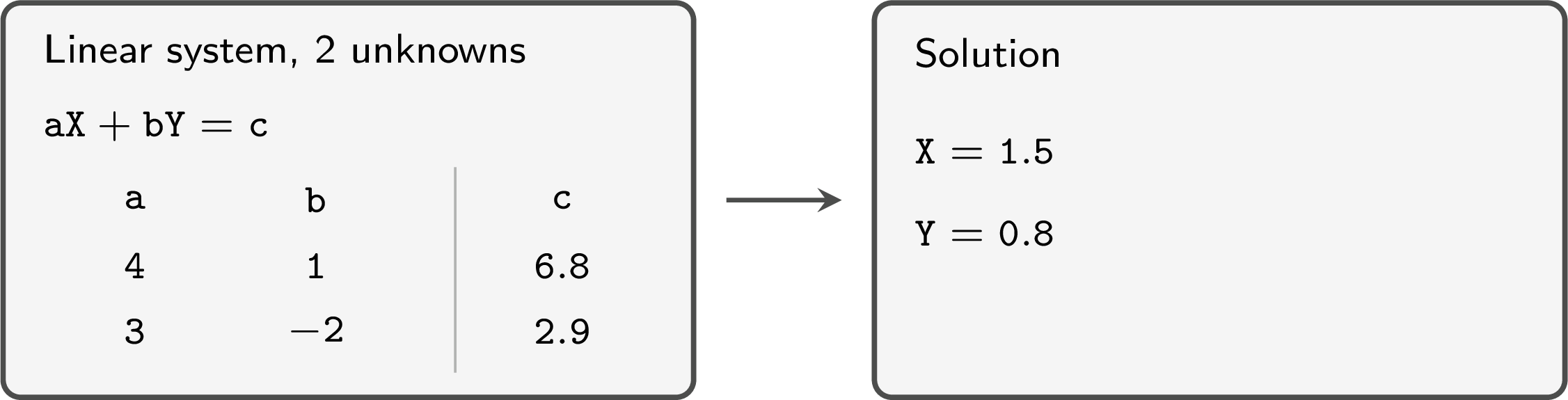
The linear system solver, in the equation menu of a graphing calculator, solves a system of two linear equations in two unknowns, or of three linear equations in three unknowns.

Write each equation in the form $ax + by = c$ (two unknowns) or $ax + by + cz = d$ (three unknowns): the unknowns on the left, in the same order in every equation, and the constant on the right.
Open the linear system solver and choose the number of unknowns.
Enter the coefficients row by row, one row per equation, each with its sign, and $0$ for a missing unknown.
Solve and read the value of each unknown. If the solver reports no solution, or infinitely many, the system has no unique solution.
Check the solution by substituting it in each original equation, then report each value exactly when the checks hold exactly, otherwise to 3 significant figures.

The mock-up solves $\begin{cases} 4x + y = 6.8 \\ 3x - 2y = 2.9 \end{cases}$: the solution is $x = 1.5$ and $y = 0.8$. Check: $4 \times 1.5 + 0.8 = 6.8$ and $3 \times 1.5 - 2 \times 0.8 = 2.9$, exactly, so these values are exact.

Skills to practice

Finding the Parameters of a Model

III Cubic Models

Definition — Cubic Model

A cubic model is a function of the form$$ f(x)=ax^3+bx^2+cx+d, \qquad a\neq 0. $$

$a$ fixes the end behaviour of the graph: its sign tells whether the curve rises to the right ($a > 0$) or falls to the right ($a < 0$).
$d$ is the $y$-intercept, since $f(0)=d$.

Example

The vertical height of a child above the ground, $h$ metres, as they go down a water slide can be modelled by the function$$h(t) = \frac{4}{7}(35 - 12t + 6t^2 - t^3),$$ where $t$ is the time in seconds after the child enters the slide.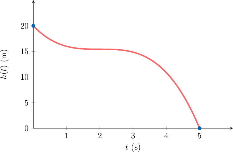

State the vertical height of the slide.
Given that the child reaches the ground at the bottom of the slide, find the domain of the function.

Answer

The height of the slide is the initial height at $t=0$.$$ h(0) = \frac{4}{7}(35) = 20 \text{ m}. $$
The child reaches the ground when $h(t) = 0$.$$ \frac{4}{7}(35 - 12t + 6t^2 - t^3) = 0 \implies 35 - 12t + 6t^2 - t^3 = 0. $$ Using a calculator or inspection, $t=5$ is a root:$$ 35 - 12(5) + 6(25) - 125 = 35 - 60 + 150 - 125 = 0. $$ Since the child starts at $t=0$ and reaches the ground at $t=5$, the physically meaningful domain is $0 \le t \le 5$.

Skills to practice

Finding a Cubic Model through Given Points

IV Going further

Skills to practice

Reasoning about Variation Models
Solving Problems with Cubic Models
Quiz

\(v\)	\(2\)	\(4\)	\(6\)	\(8\)
\(R\)	\(1.2\)	\(4.8\)	\(10.8\)	\(19.2\)

\(w\)	\(2\)	\(3\)	\(4\)	\(6\)
\(T\)	\(18\)	\(12\)	\(9\)	\(6\)

\(v\)	\(2\)	\(4\)	\(6\)	\(8\)
\(\frac{R}{v}\)	\(0.6\)	\(1.2\)	\(1.8\)	\(2.4\)
\(\frac{R}{v^2}\)	\(0.3\)	\(0.3\)	\(0.3\)	\(0.3\)