International Baccalaureate · DP 1: Applications and Interpretation SL
Functions
I
Functions and Their Graphs
I.1
What Is a Function?
Recappreviously studied — click to reread
A function is like a machine that follows a specific rule. For every number you put in, you get exactly one number out.
Consider a machine whose rule is "multiply by 2". 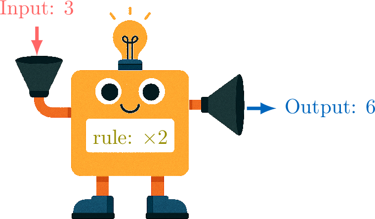
If we put in a 3, we get out a 6. If we put in a 5, we get out a 10. A table of values helps us organize these pairs:
To work with these rules more efficiently, mathematicians developed a special notation.
To represent this machine, we write \(\textcolor{olive}{f}(\textcolor{colordef}{\text{input}}) = \textcolor{colorprop}{\text{output}}\). The parentheses \((\) \()\) indicate the action of the function \(\textcolor{olive}{f}\) on the input.
We use function notation to name functions and their variables, replacing "\(\textcolor{colordef}{\text{input}}\)" by "\(\textcolor{colordef}{x}\)" and "\(\textcolor{colorprop}{\text{output}}\)" by "\(\textcolor{colorprop}{f(x)}\)".
A function maps every element from a set of inputs, the domain \(X\), to an element in a set of possible outputs, the codomain \(Y\). This is written as \(f: X \to Y\). The specific rule that maps an individual element \(x\) from the domain to an element \(f(x)\) in the codomain is written as \(x \mapsto f(x)\).
In general we write $$\Function{\textcolor{olive}{f}}{\textcolor{colordef}{X}}{\textcolor{colorprop}{Y}}{\textcolor{colordef}{x}}{\textcolor{colorprop}{f(x)}}$$ For example, if the rule is "twice the input" and we are mapping real numbers to real numbers, \(f: \mathbb{R} \to \mathbb{R}\): 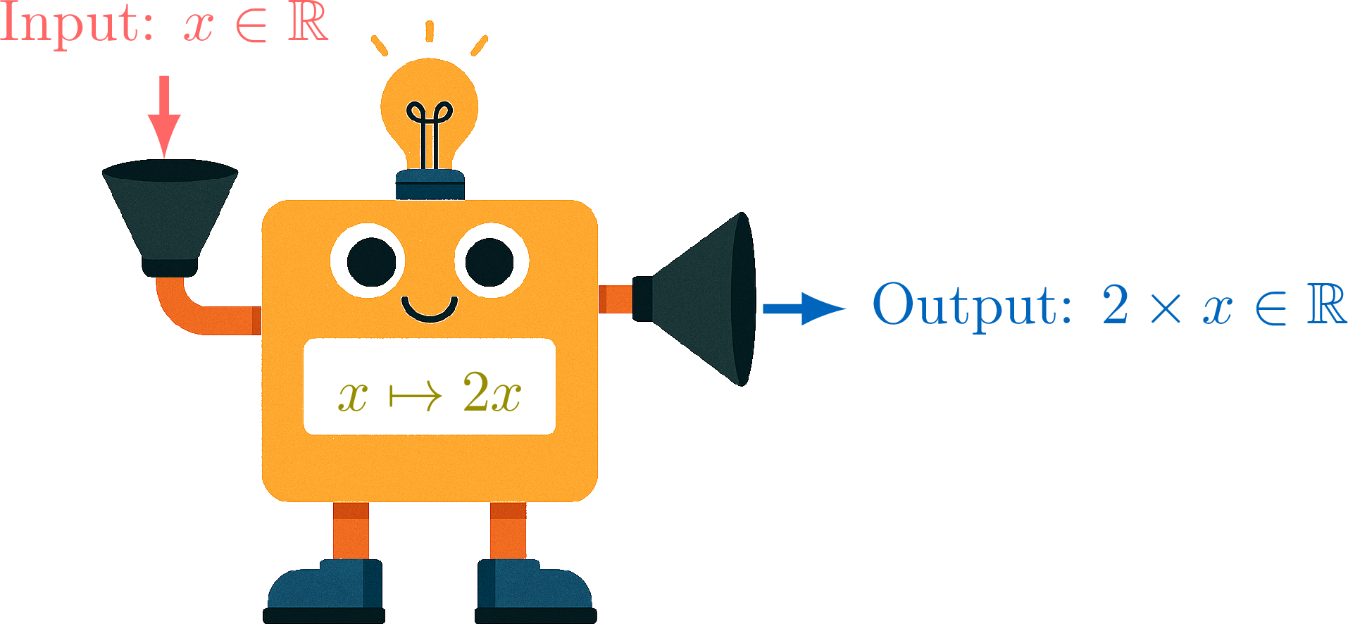
we have \(\textcolor{olive}{f}(\textcolor{colordef}{x}) = \textcolor{colorprop}{2x}\), which is written in full as:$$\Function{\textcolor{olive}{f}}{\textcolor{colordef}{\mathbb{R}}}{\textcolor{colorprop}{\mathbb{R}}}{\textcolor{colordef}{x}}{\textcolor{colorprop}{2x}}$$ When the input is \(\textcolor{colordef}{x} = \textcolor{colordef}{1}\), we get:$$\begin{aligned}\textcolor{olive}{f}(\textcolor{colordef}{1}) &= 2 \times \textcolor{colordef}{(1)}\\
&= \textcolor{colorprop}{2}\end{aligned}$$
Consider a machine whose rule is "multiply by 2".
| Input | 3 | 5 | 8 | 10 |
| Output | 6 | 10 | 16 | 20 |
To represent this machine, we write \(\textcolor{olive}{f}(\textcolor{colordef}{\text{input}}) = \textcolor{colorprop}{\text{output}}\). The parentheses \((\) \()\) indicate the action of the function \(\textcolor{olive}{f}\) on the input.
We use function notation to name functions and their variables, replacing "\(\textcolor{colordef}{\text{input}}\)" by "\(\textcolor{colordef}{x}\)" and "\(\textcolor{colorprop}{\text{output}}\)" by "\(\textcolor{colorprop}{f(x)}\)".
A function maps every element from a set of inputs, the domain \(X\), to an element in a set of possible outputs, the codomain \(Y\). This is written as \(f: X \to Y\). The specific rule that maps an individual element \(x\) from the domain to an element \(f(x)\) in the codomain is written as \(x \mapsto f(x)\).
In general we write $$\Function{\textcolor{olive}{f}}{\textcolor{colordef}{X}}{\textcolor{colorprop}{Y}}{\textcolor{colordef}{x}}{\textcolor{colorprop}{f(x)}}$$ For example, if the rule is "twice the input" and we are mapping real numbers to real numbers, \(f: \mathbb{R} \to \mathbb{R}\):
Definition — Function
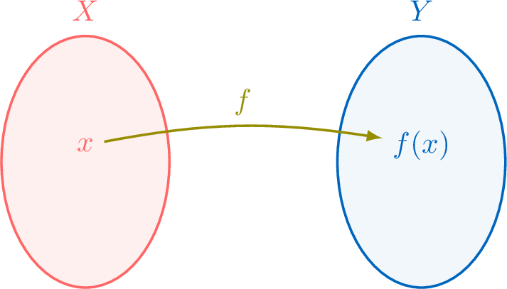
A function \(f: X \to Y\) is a rule that assigns to each element \(x\) in a set \(X\) exactly one element \(f(x)\) in a set \(Y\). - The set \(X\) of all possible inputs is called the domain of \(f\).
- The set \(Y\) is called the codomain of \(f\).
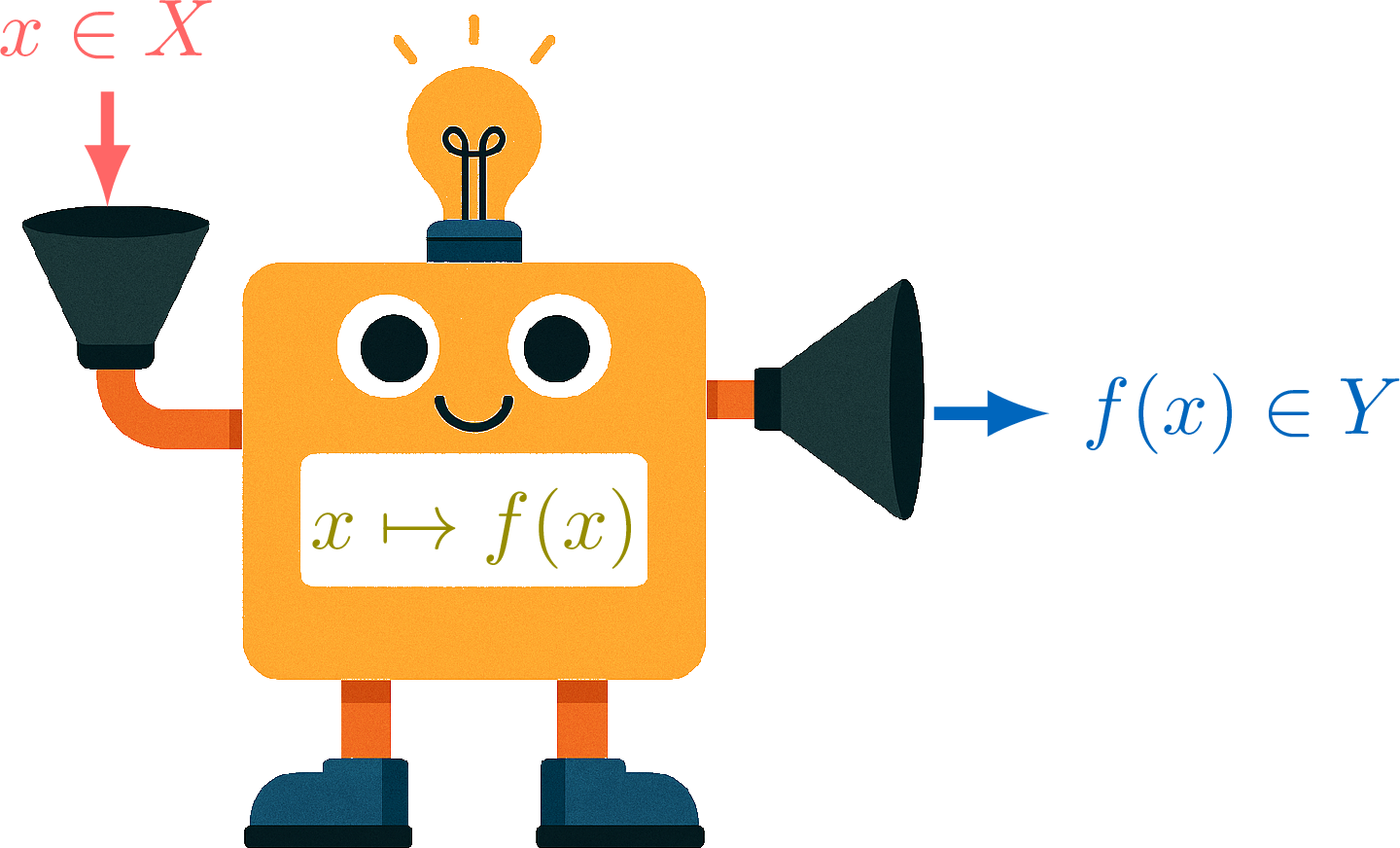
- \(f\) is the name of the function.
- \(x\) is the input variable, an element from the domain.
- \(f(x)\) is the output value in the codomain when the input is \(x\). It is read as "\(f\) of \(x\)".
- \(f(x)\) is the image of \(x\) under \(f\).
- \(x\) is a preimage of \(y=f(x)\).
Example
Let the function \(\Function{f}{\mathbb{R}}{\mathbb{R}}{x}{2x-1}\). Find the image of \(5\) under \(f\).
To find \(f(5)\), we substitute the input value \(x=5\) into the function's rule:$$\begin{aligned}[t]f(5) &= 2(5) - 1 \\
&= 10 - 1 \\
&= \boldsymbol{9}\end{aligned}$$
Method — Finding Inputs from Outputs Algebraically
To find the preimage(s) of a value \(y\) for a function \(f(x)\): - Set the function's formula equal to the output value: \(\boldsymbol{f(x) = y}\).
- Solve the resulting equation for \(x\).
Example
Let \(f(x) = 3x + 12\). Find all values of \(x\) such that \(f(x)=0\).
We need to find the value of \(x\) such that \(f(x)=0\). We set up the equation and solve: $$\begin{aligned} f(x) &= 0 \\
3x + 12 &= 0 \\
3x &= -12 && \color{gray}\text{(subtract 12 from both sides)} \\
x &= \frac{-12}{3} &&\color{gray}\text{(divide both sides by 3)} \\
x &= -4 \end{aligned}$$ The preimage of \(0\) is \(\boldsymbol{x = -4}\).
Check: \(f(-4) = 3(-4) + 12 = -12 + 12 = 0\). The answer is correct.
Check: \(f(-4) = 3(-4) + 12 = -12 + 12 = 0\). The answer is correct.
Skills to practice
- Finding Preimages
I.2
Domain and Range
Recappreviously studied — click to reread
Definition — Range
The range of a function \(f:X\to Y\) is the set of all actual output values produced by the function. It is the set of all images of the elements in the domain.$$ \text{Range} = f(X)=\{f(x):x\in X\} $$ The range is a subset of the codomain (\(f(X) \subseteq Y\)). While the codomain is the set of potential outputs, the range is the set of actual outputs. 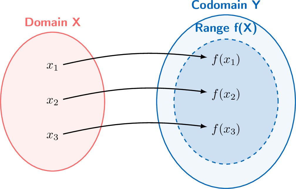
Example
For the function \(\Function{f}{\mathbb{R}}{\mathbb{R}}{x}{x^2}\): - The domain is \(\mathbb{R}\) (all real numbers).
- The codomain is also \(\mathbb{R}\).
- However, since \(x^2\geq 0\), the range is \([0, \infty)\), which is a subset of the codomain.
Definition — Natural Domain
When a function is given by a formula and the domain is not explicitly specified, the natural domain is the largest set of real numbers for which the formula yields a defined real number.
Note
When a function's rule is given without explicitly specifying the domain and codomain, we assume the natural domain as the domain and the set of all real numbers, \(\mathbb{R}\), as the codomain.
For example, when we write \(f:x\mapsto \sqrt{x}\), we implicitly assume the domain is the set of non-negative real numbers, \([0, \infty)\), and the codomain is \(\mathbb{R}\). Thus, it is shorthand for \(\Function{f}{[0, \infty)}{\mathbb{R}}{x}{\sqrt{x}}\).
Sometimes, we simply refer to "the function \(\sqrt{x}\)". This is also a shorthand for the function defined on its natural domain.
Method — Finding the Natural Domain
To find the natural domain of a function, we assume the domain is all real numbers (\(\mathbb{R}\)) and then exclude any values of \(x\) that would lead to an undefined mathematical operation. The restrictions looked for are caused by: - Rational Functions: The denominator of a fraction cannot be zero. We solve
denominator = 0to find values to exclude. - Even Roots: The expression inside an even root (like a square root, \(\sqrt{\cdot}\), or fourth root, \(\sqrt{\cdot}\)) must be non-negative (\(\ge 0\)).
- Logarithms: The argument of a logarithm must be strictly positive (\(> 0\)).
Example
Find the natural domain of the function \(f:x\mapsto\frac{1}{x-2}\).
The function involves division. Division is undefined when the denominator is zero. Therefore, we must exclude any value of \(x\) that makes the denominator \(x-2\) equal to zero.
Set the denominator to zero and solve for \(x\):$$x-2 = 0 \Leftrightarrow x=2$$ The natural domain is the set of all real numbers except \(2\). Using set notation, we write:$$\text{Domain} = \{x \in \mathbb{R} \mid x \neq 2\} \quad \text{or} \quad \mathbb{R} \setminus \{2\}$$ In interval notation, this is \((-\infty, 2) \cup (2, \infty)\).
Set the denominator to zero and solve for \(x\):$$x-2 = 0 \Leftrightarrow x=2$$ The natural domain is the set of all real numbers except \(2\). Using set notation, we write:$$\text{Domain} = \{x \in \mathbb{R} \mid x \neq 2\} \quad \text{or} \quad \mathbb{R} \setminus \{2\}$$ In interval notation, this is \((-\infty, 2) \cup (2, \infty)\).
Skills to practice
- Recognising a Natural Domain
- Finding the Natural Domain and the Range
I.3
Graphs of Functions
Recappreviously studied — click to reread
While a table of values is useful for listing some input–output pairs of a function, a graph is a powerful tool for visualising how the output changes when the input changes. A graph gives us a picture of the function's behaviour.
Definition — Graph of a Function
The graph of a function \(f\) is the set of all points with coordinates \((x, f(x))\) plotted on a coordinate plane. The input, \(x\), is plotted on the horizontal axis (the x-axis), and the output, \(f(x)\), is plotted on the vertical axis (the y-axis). When we connect these points, we form the curve of the function.$$\text{Graph of } f = \{(x,f(x)): x \in X\}$$ 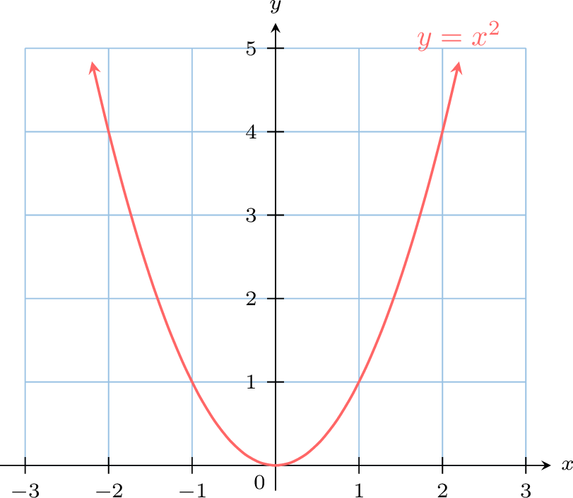
Method — Plotting a Graph from a Table
To plot the graph of a function from its table of values: - Draw a coordinate plane with a suitable scale on each axis and label the axes.
- For each pair \((x, f(x))\) in the table, plot the corresponding point on the coordinate plane.
- If the function is defined for all \(x\) in the interval shown, connect the points with a straight line or a smooth curve.
Method — Finding the Value of \(f(x)\) from a Graph
To find the output \(f(x)\) for a given input \(x\) using a graph: - Locate the input value on the horizontal x-axis.
- Move vertically from that point to the curve of the function.
- Move horizontally from the intersection point to the vertical y-axis and read the corresponding value. This y-value is the output \(f(x)\).
Example
Using the graph of the function \(f\) below, find the value of \(f(2)\). 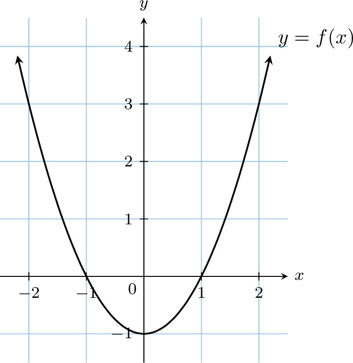
We follow the graphical method: 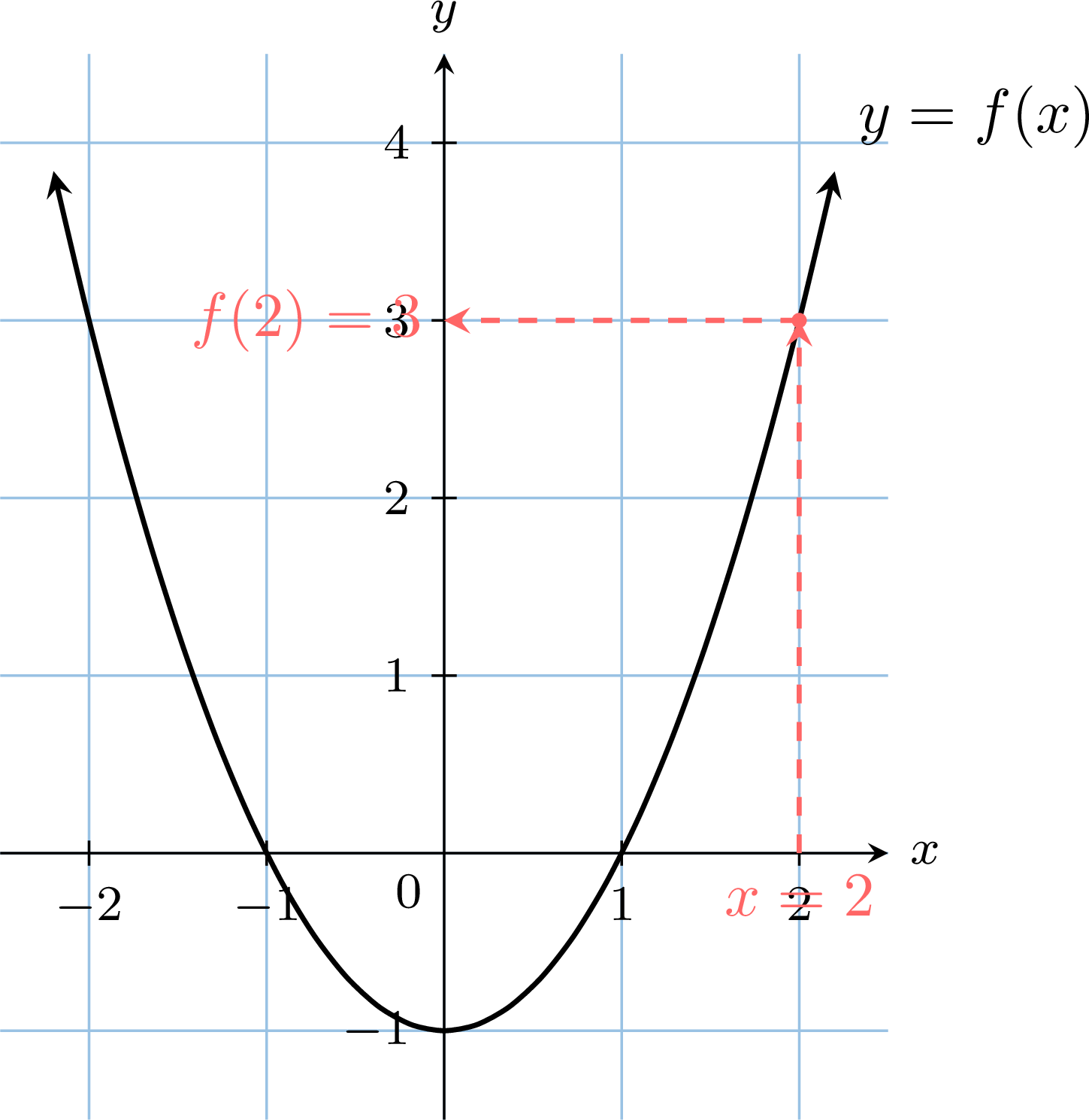
Therefore, \(\boldsymbol{f(2) = 3}\).
- Start at \(x=2\) on the horizontal axis.
- Move up to meet the curve.
- Move horizontally to the vertical axis and read the value, which is \(3\).
Method — Finding Inputs from Outputs on a Graph
To find the preimage(s) of a value \(y\) (i.e., find all \(x\) such that \(f(x)=y\)): - Locate the output value \(y\) on the vertical y-axis.
- Draw a horizontal line from this value across the graph.
- Find the intersection point(s) where the horizontal line crosses the function's curve.
- Move vertically to the x-axis from each intersection point to read the corresponding input value(s). These are the preimages.
Example
Using the graph of the function \(f\) below, find all values of \(x\) such that \(f(x)= 3\).
We apply the graphical method: 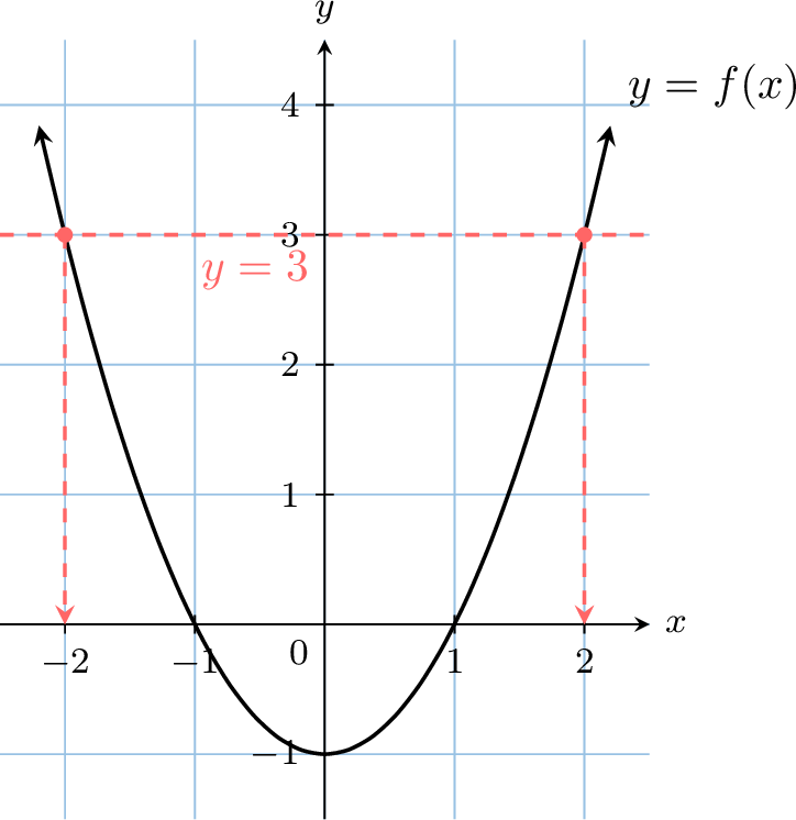
The preimages of \(3\) are \(\boldsymbol{-2}\) and \(\boldsymbol{2}\).
- We locate \(y=3\) on the vertical axis.
- We draw a horizontal line at \(y=3\).
- The line intersects the curve at two points.
- We move vertically from these points to the x-axis to read the values, which are \(-2\) and \(2\).
Skills to practice
- Finding Inputs from Outputs on a Graph
I.4
The Sign of a Function
Recappreviously studied — click to reread
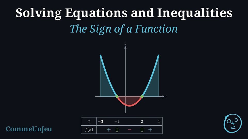
Definition — Sign of a Function
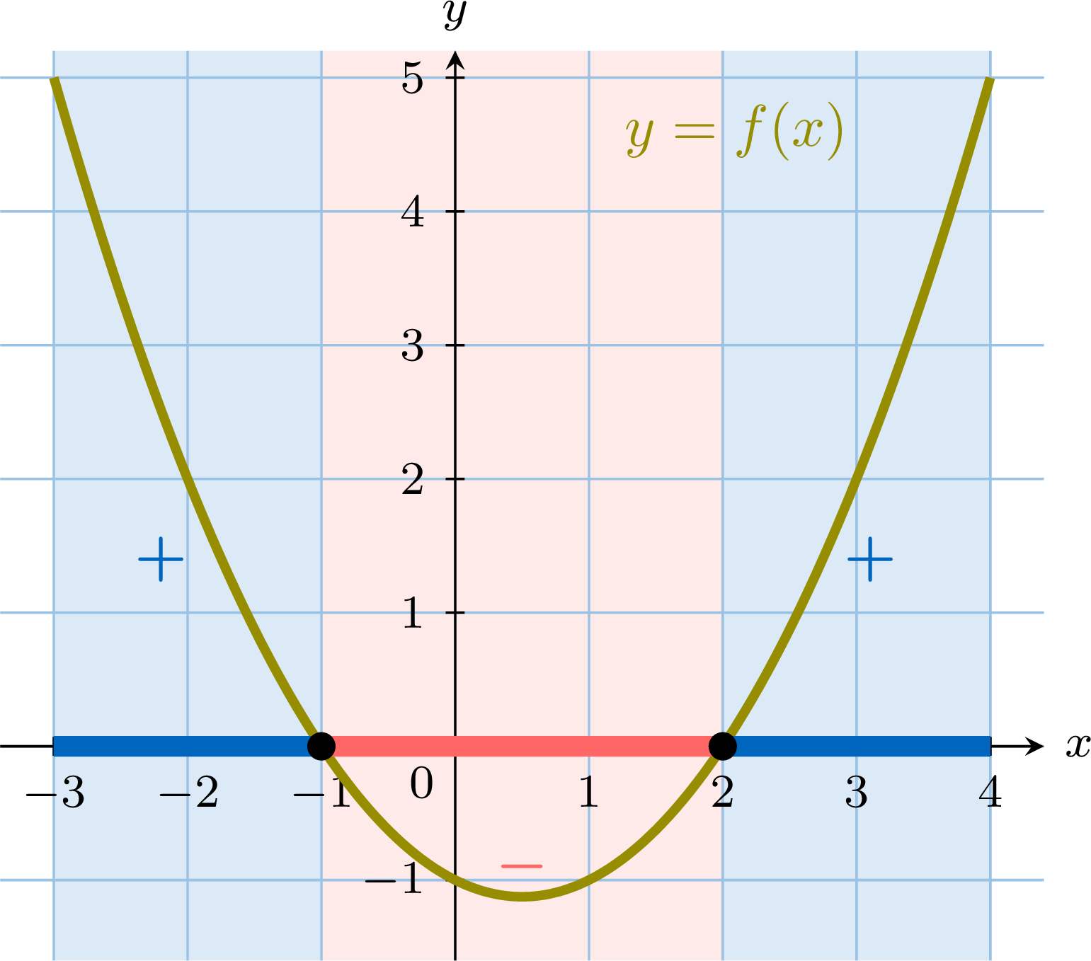
Let \(f\) be a function defined on a set \(D\) and \(I\) an interval contained in \(D\). - \(f\) is non-negative on \(I\) if \(f(x) \geq 0\) for every \(x\) in \(I\): the curve is on or above the \(x\)-axis.
- \(f\) is non-positive on \(I\) if \(f(x) \leq 0\) for every \(x\) in \(I\): the curve is on or below the \(x\)-axis.
Method — Reading the Sign of a Function from its Curve
- Mark the points where the curve meets the \(x\)-axis: at these values, \(f\) vanishes (\(f(x) = 0\)).
- Where the curve is above the axis, \(f(x) \gt 0\); where it is below, \(f(x) \lt 0\).
- Summarise in a sign table: the values where \(f\) vanishes in the top row, the symbols \(+\), \(0\) and \(-\) in the bottom row.
Example
The function \(f\) of the definition above is drawn on \([-3, 4]\), and vanishes at \(-1\) and \(2\). Construct the sign table of \(f\).
The curve is above the axis before \(-1\), below between \(-1\) and \(2\), above after \(2\): 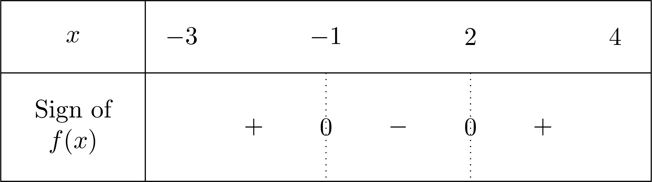
Skills to practice
- The Sign of a Function
I.5
Graphs with Technology
Method — Reading the Key Features of a Graph on the Screen
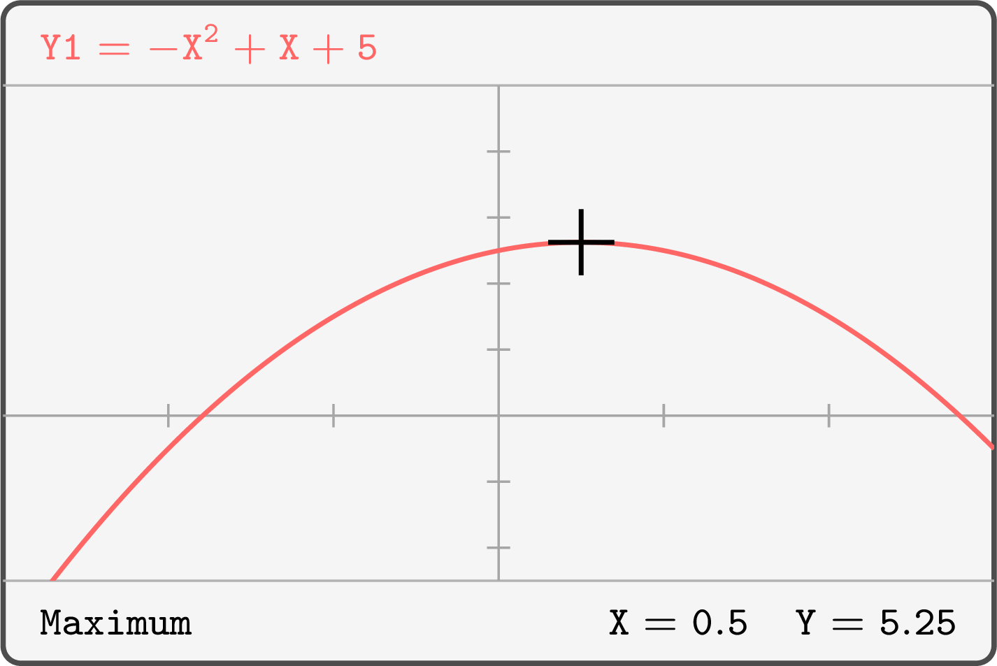
To study the graph of a function \(f\) with a graphing calculator: - Enter \(f(x)\) as the first function (\(Y_1\)) of the function editor.
- Choose the window: the least and greatest values of \(x\) and of \(y\) shown on the screen. Start from the domain the question gives, or from a table of values of \(f\), and adjust until every feature asked for is visible. A window that is too narrow hides an intercept or a turning point; a window that is too wide flattens the curve.
- Read each feature with the analysis tools of the graph menu, never by eye:
- the \(y\)-intercept: the value of \(f\) at \(x = 0\);
- each \(x\)-intercept: the tool zero (or root);
- a local maximum or minimum: the tool maximum or minimum, which gives both coordinates of the turning point.
Example
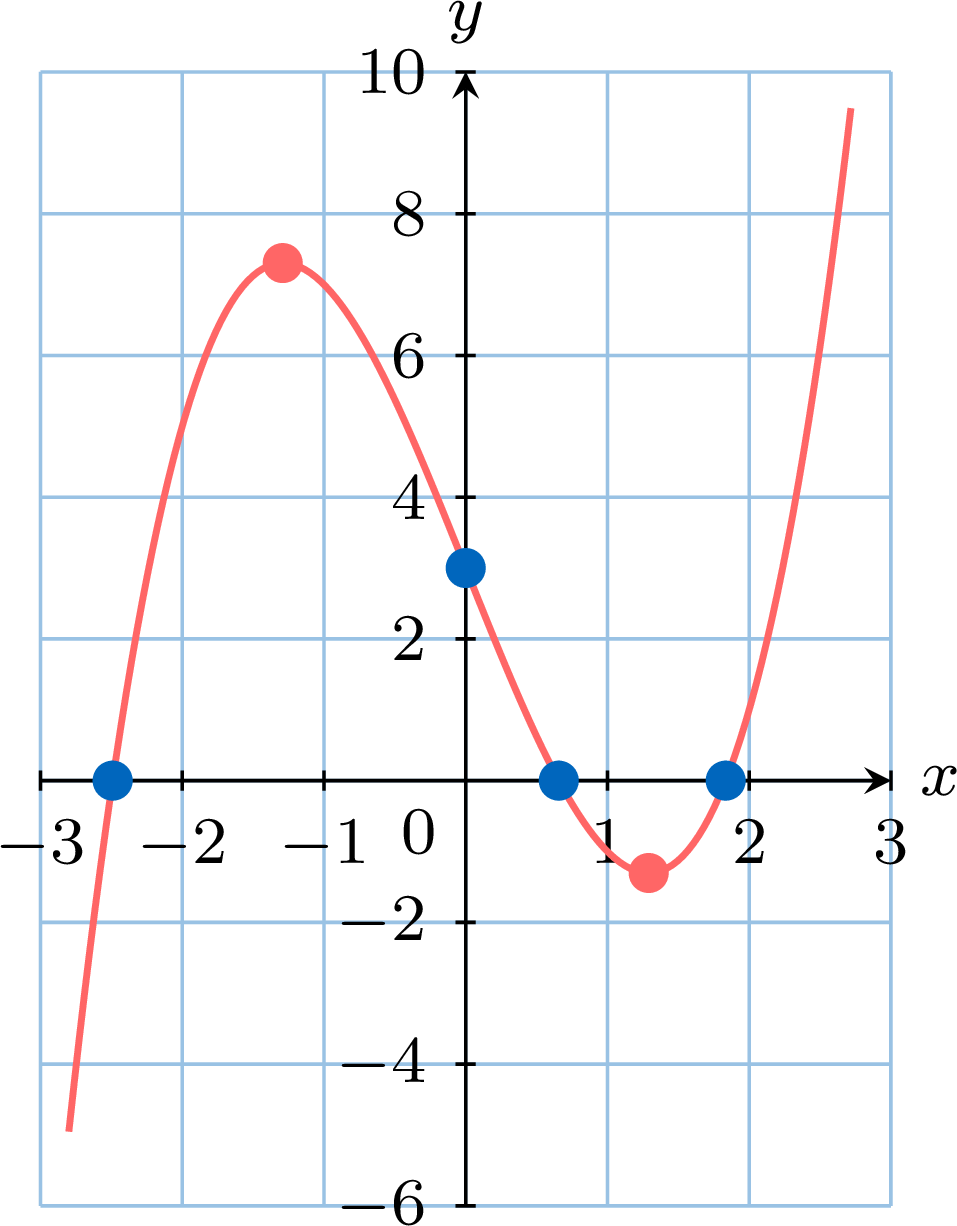
Let \(f(x) = x^3 - 5x + 3\). - Choose a window that shows the intercepts and the turning points of the graph of \(f\).
- Find the \(y\)-intercept and the \(x\)-intercepts of the graph.
- Find the local maximum point and the local minimum point.
- A table of values of \(f(x) = x^3 - 5x + 3\) at the integers guides the choice:
\(x\) \(-3\) \(-2\) \(-1\) \(0\) \(1\) \(2\) \(3\) \(f(x)\) \(-9\) \(5\) \(7\) \(3\) \(-1\) \(1\) \(15\) - The \(y\)-intercept is \(f(0) = 3\). The zero tool, bounded between \(-3\) and \(-2\), then between \(0\) and \(1\), then between \(1\) and \(2\), displays \(-2.4908636\), \(0.6566204\) and \(1.8342432\): the \(x\)-intercepts are \(x \approx -2.49\), \(x \approx 0.657\) and \(x \approx 1.83\). An equation of degree \(3\) has at most three real roots, so none is missing.
- The maximum tool, bounded between \(-2\) and \(0\), displays \(X = -1.2909944\) and \(Y = 7.3033148\); the minimum tool, bounded between \(0\) and \(2\), displays \(X = 1.2909944\) and \(Y = -1.3033148\). The local maximum point is \((-1.29, 7.30)\) and the local minimum point is \((1.29, -1.30)\).
Example
Let \(g(x) = \dfrac{2x - 1}{x + 1}\), for \(x \neq -1\). Graph \(g\) with technology. Give the intercepts of the graph and the equations of the asymptotes that the screen suggests, then confirm each asymptote with the formula.
The graph of \(g(x) = \dfrac{2x - 1}{x + 1}\), in the window \(-6 \le x \le 4\), \(-4 \le y \le 8\), shows two branches, one on each side of the vertical line \(x = -1\); both flatten towards the horizontal line \(y = 2\). 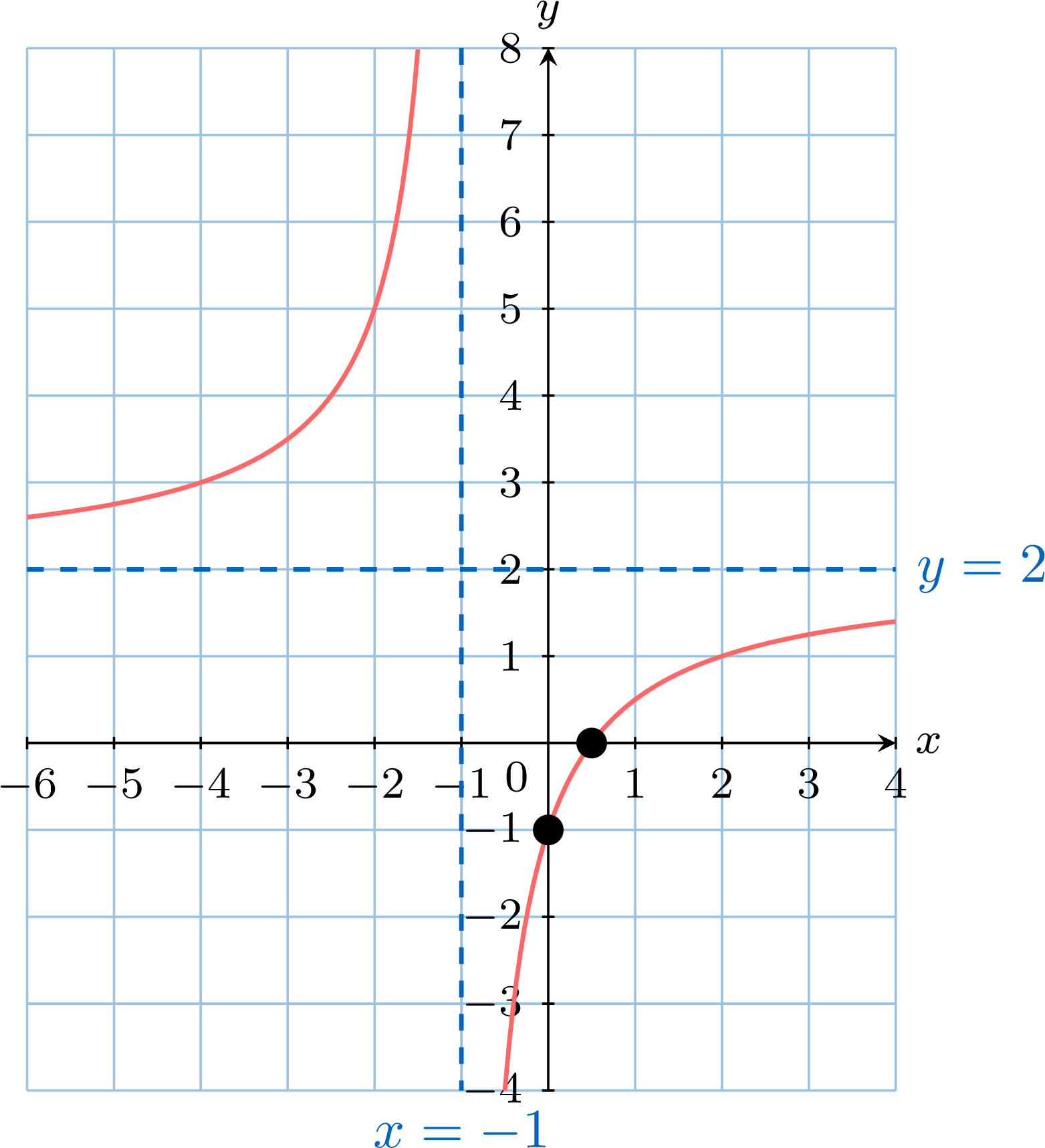
- Intercepts. The value of \(g\) at \(0\) is \(g(0) = \dfrac{-1}{1} = -1\): the \(y\)-intercept is \(-1\). The zero tool displays \(X = 0.5\), an exact value, since \(2x - 1 = 0\) for \(x = \dfrac{1}{2}\): the \(x\)-intercept is \(0.5\).
- Vertical asymptote. The denominator \(x + 1\) is zero for \(x = -1\), while the numerator equals \(-3 \neq 0\) there: the line \(x = -1\) is a vertical asymptote.
- Horizontal asymptote. The numerator is rewritten around the denominator: $$\begin{aligned}[t] g(x) &= \frac{2(x + 1) - 3}{x + 1} &&\text{(}2x - 1 = 2(x + 1) - 3\text{)} \\ &= 2 - \frac{3}{x + 1}. &&\text{(divide each term by } x + 1\text{)} \end{aligned}$$ When \(x\) is large, positive or negative, the fraction \(\dfrac{3}{x + 1}\) is as small as desired, so \(g(x)\) is as close to \(2\) as desired: the line \(y = 2\) is a horizontal asymptote.
Skills to practice
- Reading Key Features with Technology
- Studying Graphs with Technology
I.6
Injective, Surjective and Bijective Functions
For a function to be perfectly reversible (i.e., to have an inverse), it must create a perfect pairing between the elements of its domain and its codomain. This leads to the concept of a bijection, which is a function that is both injective and surjective.
Definition — Injective, Surjective, and Bijective Functions
Let \(f: X \to Y\) be a function. - \(f\) is injective (one-to-one) if different inputs produce different outputs. For any \(x_1, x_2 \in X\), if \(x_1 \neq x_2\), then \(f(x_1) \neq f(x_2)\).
- \(f\) is surjective (onto) if its range is equal to its codomain (\(f(X)=Y\)). This means every element in the codomain \(Y\) is the image of at least one element from the domain \(X\).
- \(f\) is bijective if it is both injective and surjective. This means every element in the codomain is the image of exactly one element from the domain.
Example
Consider two versions of the squaring function: - \(\Function{f}{\mathbb{R}}{\mathbb{R}}{x}{x^2}\)
- \(\Function{g}{[0,\infty)}{[0,\infty)}{x}{x^2}\)
- The function \(f\) is not bijective. It is not injective because \(f(-2)=f(2)\). It is not surjective because its range, \([0, \infty)\), is not equal to its codomain, \(\mathbb{R}\).
- The function \(g\) is bijective. It is injective because its domain is restricted to non-negative numbers. It is surjective because its range, \([0, \infty)\), is equal to its specified codomain, \([0, \infty)\).
Method — The Horizontal Line Test for Bijectivity
To determine visually if a function \(f: X \to Y\) is bijective: - Draw the graph of the function \(f(x)\).
- Imagine drawing horizontal lines across the graph for every possible \(y\)-value in the codomain \(Y\).
- Conclusion:
- The function is bijective if and only if every horizontal line (for all \(y \in Y\)) intersects the graph exactly once.
- Intersecting at most once shows it is injective.
- Intersecting at least once shows it is surjective.
- The function is bijective if and only if every horizontal line (for all \(y \in Y\)) intersects the graph exactly once.
Example
Use the horizontal line test to determine if the function \(\Function{f}{\mathbb{R}}{\mathbb{R}}{x}{x^2}\) is a bijective function.
First, we graph the function \(f(x) = x^2\). The specified codomain is \(\mathbb{R}\). 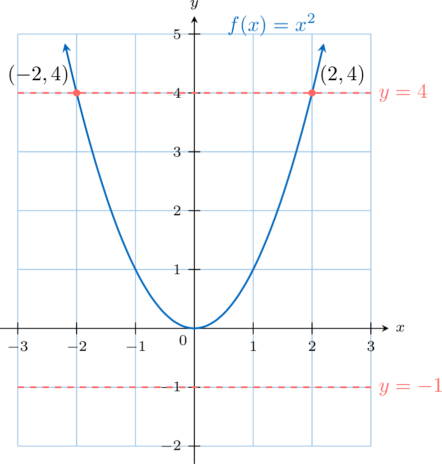
We test for both conditions:
- Injectivity: The horizontal line \(y=4\) intersects the graph at two distinct points, \((-2,4)\) and \((2,4)\). Since a horizontal line intersects the graph more than once, the function is not injective.
- Surjectivity: The horizontal line \(y=-1\) is in the codomain (\(\mathbb{R}\)) but does not intersect the graph at all. This means that \(-1\) has no preimage. Since there is an element in the codomain that is not in the range, the function is not surjective.
Skills to practice
- Deciding Whether a Function Is Injective, Surjective or Bijective
II
Operations on Functions
II.1
Sums, Differences and Products of Functions
Let \(\textcolor{colordef}{f(x)=2x+1}\) and \(\textcolor{colorprop}{g(x)=x^2}\).
\(\textcolor{olive}{(f+g)(x)}\) means that, for any input \(x\) that belongs to the domains of both functions, \(\textcolor{colordef}{f(x)}\) and \(\textcolor{colorprop}{g(x)}\) are calculated separately, then the results are added. In other words, \((f+g)\) is a new function defined by \((f+g)(x)=f(x)+g(x)\).
This is illustrated by the function machine below: 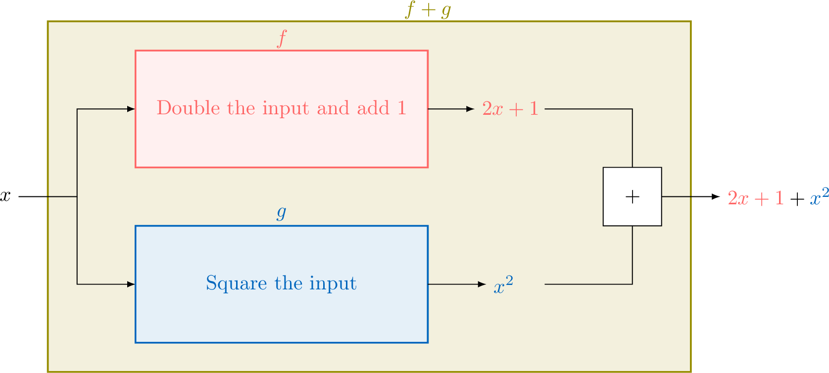
So, $$\begin{aligned}[t]\textcolor{olive}{(f+g)(x)} &= \textcolor{colordef}{f(x)} + \textcolor{colorprop}{g(x)} \\
&= \textcolor{colordef}{2x+1} + \textcolor{colorprop}{x^2}.\end{aligned}$$
\(\textcolor{olive}{(f+g)(x)}\) means that, for any input \(x\) that belongs to the domains of both functions, \(\textcolor{colordef}{f(x)}\) and \(\textcolor{colorprop}{g(x)}\) are calculated separately, then the results are added. In other words, \((f+g)\) is a new function defined by \((f+g)(x)=f(x)+g(x)\).
This is illustrated by the function machine below:
Definition — Operations on Functions
Given two functions \(f\) and \(g\), we can define new functions by performing arithmetic operations on their outputs, for each \(x\) where both are defined: - Sum: \((f+g)(x) = f(x) + g(x)\)
- Difference: \((f-g)(x) = f(x) - g(x)\)
- Product: \((fg)(x) = f(x) \times g(x)\)
- Quotient: \(\displaystyle\left(\frac{f}{g}\right)(x) = \frac{f(x)}{g(x)}\), provided that \(g(x) \neq 0\).
For the quotient, the domain is the intersection of the domains of \(f\) and \(g\), excluding any \(x\) such that \(g(x)=0\).
Example
Let \(f(x)=2x+1\) and \(g(x)=x^4-1\). Find \((f+g)(x)\).
\(\begin{aligned} (f+g)(x) &= f(x) + g(x) \\ &= (2x+1) + (x^4-1) \\ &= x^4 + 2x. \end{aligned}\)
Since both \(f\) and \(g\) are polynomials, \((f+g)(x)\) is defined for all real numbers \(x\).
Since both \(f\) and \(g\) are polynomials, \((f+g)(x)\) is defined for all real numbers \(x\).
Skills to practice
- Adding, Subtracting and Multiplying Functions
II.2
Inverse Functions
In arithmetic, we are familiar with inverse operations. For example, subtraction is the inverse of addition because it “undoes” the addition. Starting with 5, adding 3 gives 8, and subtracting 3 then returns to 5: $$(5+3) - 3 = 5.$$ Similarly, division is the inverse of multiplication: $$(5\times 3) \div 3 = 5.$$ The concept of an inverse function follows the same idea. An inverse function, denoted \(\boldsymbol{f^{-1}}\), is a function that “undoes” or reverses the action of another function, \(f\).
If a function \(f\) takes an input \(x\) to an output \(y\), the inverse function \(f^{-1}\) takes that output \(y\) back to the original input \(x\). This creates a perfect loop: 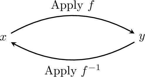
However, not every function has an inverse function. For an inverse to exist, each output \(y\) must come from exactly one input \(x\) (the function must never take the same value twice on its domain).
If a function \(f\) takes an input \(x\) to an output \(y\), the inverse function \(f^{-1}\) takes that output \(y\) back to the original input \(x\). This creates a perfect loop:
Definition — Inverse Function
Let \(f: X \to Y\) be a bijective function.The inverse function, denoted \(f^{-1}\), is the function \(\boldsymbol{f^{-1}: Y \to X}\) that reverses the action of \(f\).
This means that if \(f\) maps an input \(x\) to an output \(y\), then \(f^{-1}\) maps that output \(y\) back to the original input \(x\). This relationship is defined by:$$ f(x) = y \iff f^{-1}(y) = x $$
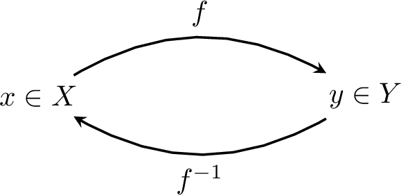
- \(\boldsymbol{(f^{-1} \circ f)(x) = x}\) for all \(x\) in the domain of \(f\) (\(X\)).
- \(\boldsymbol{(f \circ f^{-1})(y) = y}\) for all \(y\) in the domain of \(f^{-1}\) (\(Y\)).
Method — Finding the Inverse Function
To find the inverse of a function \(f\) (when it exists): - Set \(y = f(x)\).
- Solve the equation for \(x\) in terms of \(y\). This gives an expression of the form \(x = f^{-1}(y)\).
- Swap the variables \(x\) and \(y\) to write the inverse in terms of \(x\). The result is \(y = f^{-1}(x)\).
Example
Find the inverse of the function \(\Function{f}{[0,\infty)}{[0,\infty)}{x}{\sqrt{x}}\).
The function is \(f(x) = \sqrt{x}\) with Domain: \([0, \infty)\) and Range: \([0, \infty)\).
- Set \(y = \sqrt{x}\).
- Solve for \(x\): Since the domain of \(f\) is non-negative, \(x \ge 0\), and the range is non-negative, \(y \ge 0\). We can square both sides: $$ y^2 = x \Leftrightarrow x = y^2 $$
- Swap variables to get the rule: \(y = x^2\).
- The domain of \(f^{-1}\) is the range of \(f\), which is \([0, \infty)\). The range of \(f^{-1}\) is the domain of \(f\), which is \([0, \infty)\).
Proposition — Symmetry of Inverse Functions
The graph of a function \(f\) and its inverse \(f^{-1}\) are reflections of each other across the line \(\boldsymbol{y = x}\). 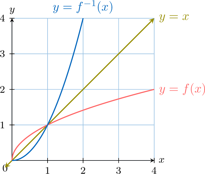
Skills to practice
- Graphing and Finding Inverse Functions
III
Going further
Skills to practice
- Reasoning and Problem-Solving
- Solving Problems on Functions
- Quiz
Jump to section