International Baccalaureate · DP 2: Analysis and Approaches HL
Properties of Curves
I
Tangents and Normals
I.1
Equation of the Tangent
The most direct geometric interpretation of the derivative is that it gives the slope of the tangent line. Finding the equation of this line is a fundamental application of differentiation.
Proposition — Equation of the Tangent
Assume \(f\) is differentiable at \(x=a\) and that the tangent is not vertical. Then the equation of the tangent to the curve \(y=f(x)\) at the point \((a, f(a))\) is:$$\textcolor{colorprop}{y = f^{\prime}(a)(x-a) +f(a)}$$ 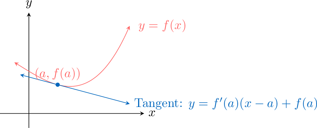
Let \(B(x,y)\) be any point on the tangent line. The point of tangency is \(A(a,f(a))\), which also belongs to the tangent line.
The gradient (also called slope) of a line is given by the formula \(m = \dfrac{\Delta y}{\Delta x}\). Using points \(A\) and \(B\), the slope of the tangent line is:$$ m = \dfrac{y-f(a)}{x-a}\quad \text{for }x\neq a. $$ By definition, the slope of the tangent to the curve \(y=f(x)\) at the point \(x=a\) is the value of the derivative at that point, so:$$ m = f'(a). $$ Equating the two expressions for the slope, we get:$$ f'(a) = \dfrac{y-f(a)}{x-a}. $$ Multiplying both sides by \((x-a)\) gives the point-gradient form (also called point-slope form) of the equation:$$ y - f(a) = f'(a)(x-a). $$ Making \(y\) the subject gives:$$ y = f'(a)(x-a) + f(a). $$
The gradient (also called slope) of a line is given by the formula \(m = \dfrac{\Delta y}{\Delta x}\). Using points \(A\) and \(B\), the slope of the tangent line is:$$ m = \dfrac{y-f(a)}{x-a}\quad \text{for }x\neq a. $$ By definition, the slope of the tangent to the curve \(y=f(x)\) at the point \(x=a\) is the value of the derivative at that point, so:$$ m = f'(a). $$ Equating the two expressions for the slope, we get:$$ f'(a) = \dfrac{y-f(a)}{x-a}. $$ Multiplying both sides by \((x-a)\) gives the point-gradient form (also called point-slope form) of the equation:$$ y - f(a) = f'(a)(x-a). $$ Making \(y\) the subject gives:$$ y = f'(a)(x-a) + f(a). $$
Example
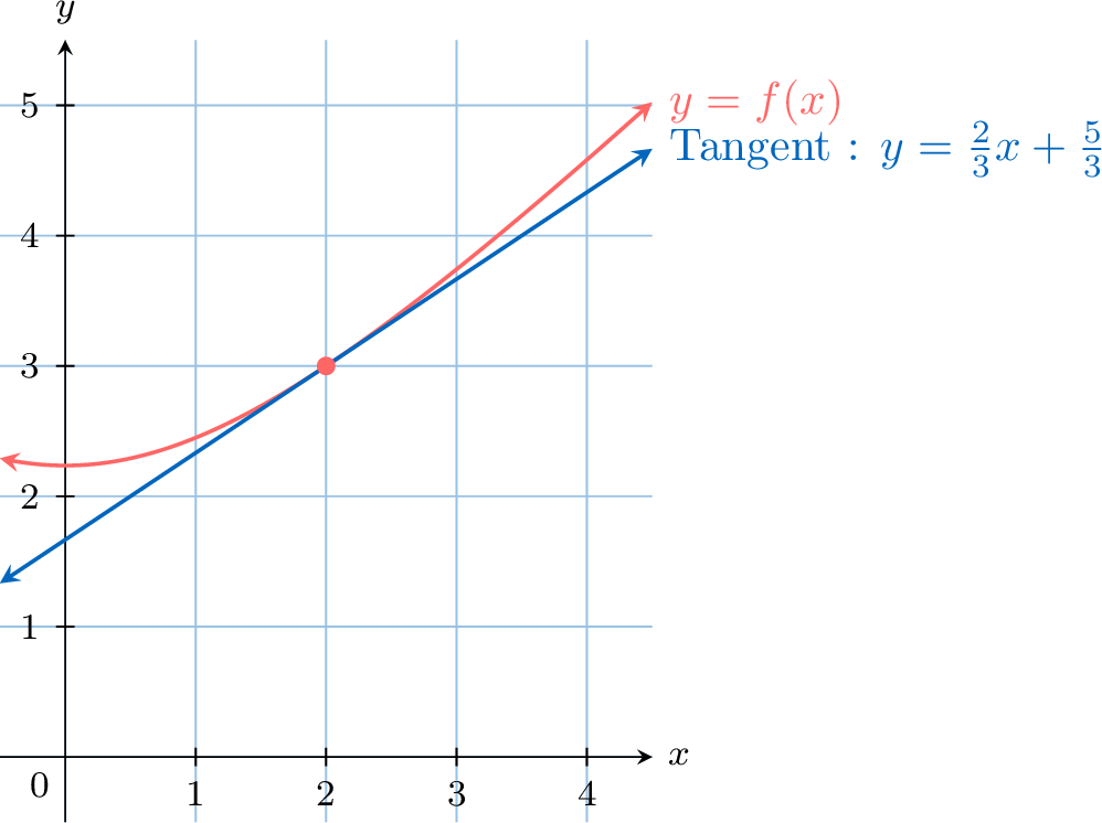
Find the equation of the tangent to \(f(x)=\sqrt{x^{2}+5}\) at \(x=2\). - Step 1: Find the derivative.
First, rewrite the function as \(f(x) = (x^2+5)^{1/2}\). Using the chain rule: $$\begin{aligned} f'(x) &= \frac{1}{2}(x^2+5)^{-1/2} \cdot (2x)\\ &= \frac{x}{\sqrt{x^2+5}}\end{aligned}$$ - Step 2: Find the coordinates of the point.
At \(x=2\), the \(y\)-coordinate is \(f(2) = \sqrt{2^2+5} = \sqrt{9} = 3\). The point is \((2,3)\). - Step 3: Find the slope of the tangent.
The slope is the value of the derivative at \(x=2\): $$ m = f'(2) = \frac{2}{\sqrt{2^2+5}} = \frac{2}{3}. $$ - Step 4: Write the equation of the line.
$$\begin{aligned} y &= f'(2)(x-2) + f(2)\\ y&=\frac{2}{3}(x-2)+3\\ y &= \frac{2}{3}x + \frac{5}{3}.\\ \end{aligned} $$
Skills to practice
- Finding the Equation of a Tangent
- Tangents at a Given Point or with a Given Gradient
I.2
The Tangent with Technology
Method — Finding the Equation of a Tangent with Technology
To find the equation of the tangent to the curve of \(f\) at the point where \(x = a\), with a graphing calculator: - Compute \(f(a)\), by substitution or with the value tool of the graph menu.
- Compute \(f'(a)\) with the derivative command, \(f\) being differentiable at \(a\), and store the full value in a memory of the calculator.
- Write the equation \(y = f'(a)(x - a) + f(a)\) and expand it to the form \(y = mx + c\) with the stored value. Round \(m\) and \(c\) only at the end, to 3 significant figures: rounding \(f'(a)\) first changes \(c\).
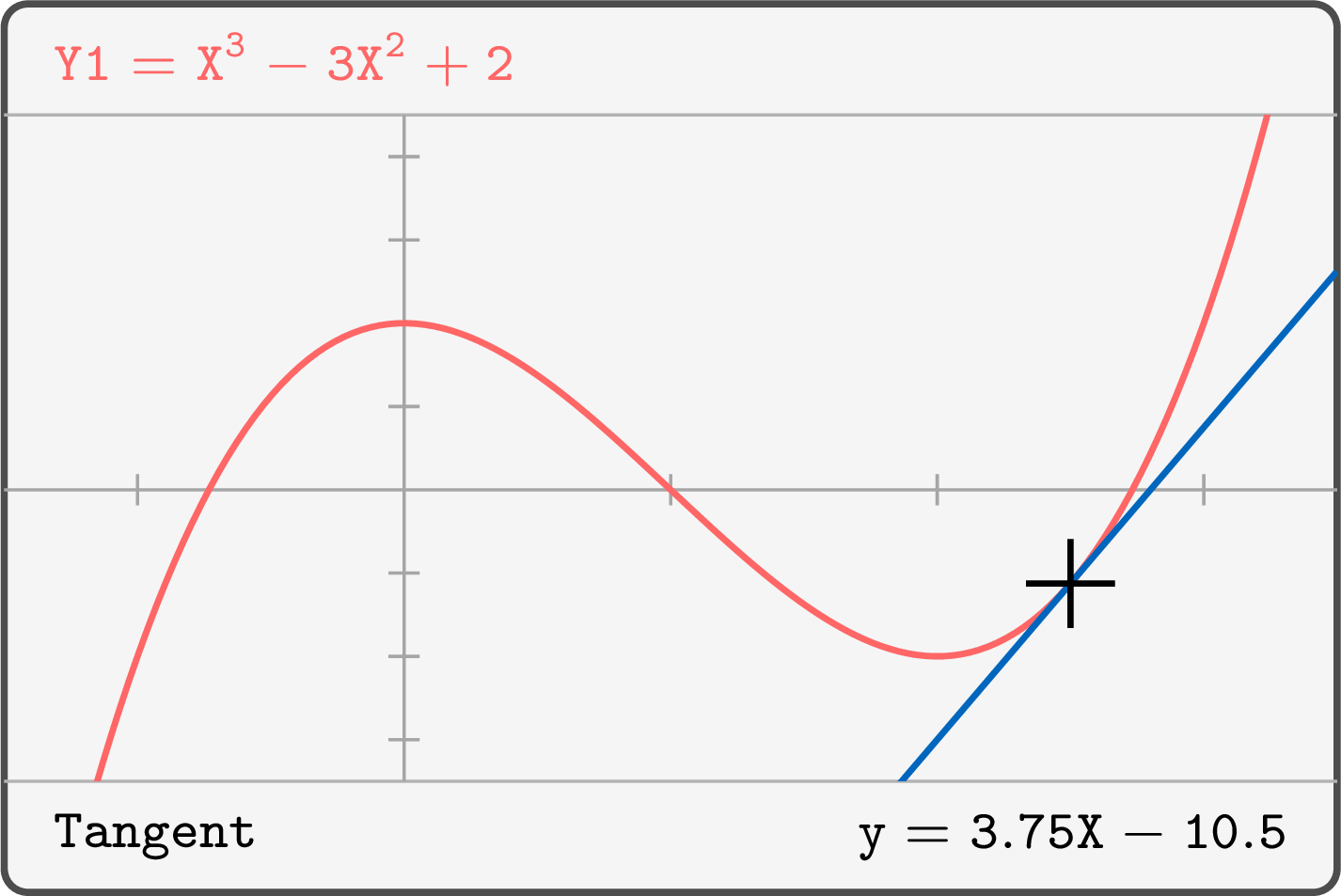
- Check on the screen: the tangent tool of the graph menu (draw or sketch menu, depending on the model), at \(x = a\), draws the tangent and displays its equation. The line must touch the curve at the point \((a, f(a))\), and its equation must match the one found.
Example
Let \(f(x) = 2^x\). Use technology to find the equation of the tangent to the curve of \(f\) at the point where \(x = 1\), in the form \(y = mx + c\) with \(m\) and \(c\) to 3 significant figures.
The point. \(f(1) = 2^1 = 2\): the point of tangency is \((1, 2)\).
The gradient. \(f\) is an exponential function, differentiable at every real number. The derivative command, with \(2^X\) and \(X = 1\), displays \(1.386294361\), stored in a memory.
The equation. $$\begin{aligned}[t] y &= f'(1)(x - 1) + f(1) &&\text{(equation of the tangent)} \\ &\approx 1.386294361(x - 1) + 2 \\ &\approx 1.386294361x + 0.613705639. &&\text{(expand)} \end{aligned}$$ Rounded at the end: \(y \approx 1.39x + 0.614\). Rounding the gradient first would give \(2 - 1.39 = 0.61\), a wrong constant. The tangent tool at \(X = 1\) draws the line through \((1, 2)\) and displays the same coefficients before rounding. 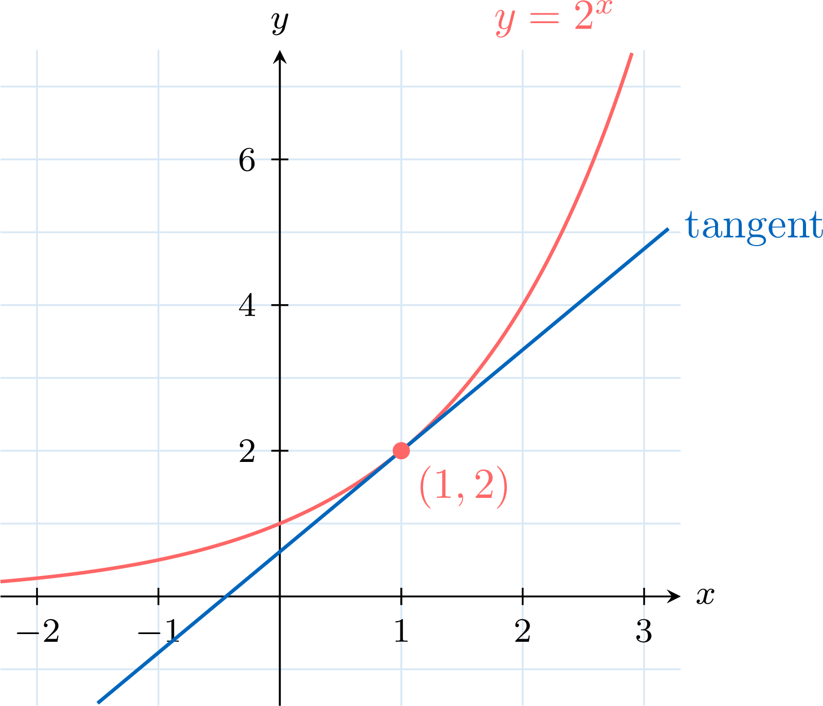
The gradient. \(f\) is an exponential function, differentiable at every real number. The derivative command, with \(2^X\) and \(X = 1\), displays \(1.386294361\), stored in a memory.
The equation. $$\begin{aligned}[t] y &= f'(1)(x - 1) + f(1) &&\text{(equation of the tangent)} \\ &\approx 1.386294361(x - 1) + 2 \\ &\approx 1.386294361x + 0.613705639. &&\text{(expand)} \end{aligned}$$ Rounded at the end: \(y \approx 1.39x + 0.614\). Rounding the gradient first would give \(2 - 1.39 = 0.61\), a wrong constant. The tangent tool at \(X = 1\) draws the line through \((1, 2)\) and displays the same coefficients before rounding.
Skills to practice
- Finding a Tangent with Technology
I.3
Equation of the Normal
Definition — Normal Line
The normal line to a curve at a point is the line that is perpendicular to the tangent line at that same point. 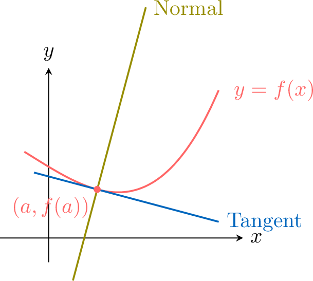
Proposition — Equation of the Normal
The equation of the normal to the curve \(y=f(x)\) at the point \((a, f(a))\) is given by: - if \(f'(a)\neq 0\), then the normal has slope \(-\dfrac{1}{f'(a)}\) and $$\textcolor{colorprop}{y = -\frac{1}{f'(a)}(x-a)+f(a)}.$$
- if \(f'(a)= 0\), then the tangent is horizontal and the normal is the vertical line \(x=a\).
- if the tangent is vertical (so its equation is \(x=a\)), then the normal is the horizontal line \(y=f(a)\).
The slope of the tangent at \(x=a\) is \(m_T = f'(a)\). Because the normal line is perpendicular to the tangent line, its slope \(m_N\) is the negative reciprocal of the tangent's slope:$$ m_N = -\frac{1}{m_T} = -\frac{1}{f'(a)} \quad (\text{provided } f'(a) \neq 0). $$ Using the point-slope form of a line with the point \((a, f(a))\) and the slope \(m_N\), we get the equation of the normal:$$ y - f(a) = -\frac{1}{f'(a)}(x-a). $$ The special cases \(f'(a)=0\) (horizontal tangent) and vertical tangent are handled as described in the statement above.
Example
Find the equation of the normal to \(f(x)=\sqrt{x^{2}+5}\) at \(x=2\). - Step 1: Find the derivative.
Using the chain rule: $$\begin{aligned} f'(x) &= \frac{1}{2}(x^2+5)^{-1/2} \cdot (2x)\\ &= \frac{x}{\sqrt{x^2+5}}\end{aligned}$$ - Step 2: Find the coordinates of the point.
At \(x=2\), the \(y\)-coordinate is \(f(2) = \sqrt{2^2+5} = \sqrt{9} = 3\). The point is \((2,3)\). - Step 3: Find the slope of the normal.
First, find the slope of the tangent at \(x=2\): $$ m_T = f'(2) = \frac{2}{\sqrt{2^2+5}} = \frac{2}{3}. $$ The slope of the normal is the negative reciprocal: $$ m_N = -\frac{1}{m_T} = -\frac{3}{2}. $$ - Step 4: Write the equation of the normal line. $$\begin{aligned} y &= -\frac{3}{2}(x-2) +3\\ y &= -\frac{3}{2}x + 6. \end{aligned} $$

Example
Let \(f(x) = 3^x\). Use technology to find the equation of the normal to the curve of \(f\) at the point where \(x = 1\), in the form \(y = mx + c\) with \(m\) and \(c\) to 3 significant figures.
The point. \(f(1) = 3^1 = 3\): the point is \((1, 3)\).
The gradient of the tangent. The derivative command, with \(3^X\) and \(X = 1\), displays about \(3.29584\) (the last digits depend on the model), kept in a memory. It is not zero, so the normal is not vertical, and its gradient is $$-\frac{1}{f'(1)} \approx -0.30341.$$ The equation of the normal. $$\begin{aligned}[t] y &= -\frac{1}{f'(1)}(x - 1) + f(1) &&\text{(equation of the normal)} \\ &\approx -0.30341(x - 1) + 3 \\ &\approx -0.30341x + 3.30341. &&\text{(expand)} \end{aligned}$$ Rounded at the end: \(y \approx -0.303x + 3.30\). Some calculators draw the normal directly (normal tool of the sketch menu) and display its equation: a check. On the screen, as on the figure, the normal looks perpendicular to the tangent only when both axes have the same unit. 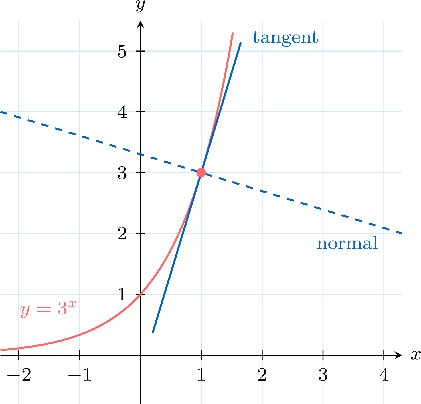
The gradient of the tangent. The derivative command, with \(3^X\) and \(X = 1\), displays about \(3.29584\) (the last digits depend on the model), kept in a memory. It is not zero, so the normal is not vertical, and its gradient is $$-\frac{1}{f'(1)} \approx -0.30341.$$ The equation of the normal. $$\begin{aligned}[t] y &= -\frac{1}{f'(1)}(x - 1) + f(1) &&\text{(equation of the normal)} \\ &\approx -0.30341(x - 1) + 3 \\ &\approx -0.30341x + 3.30341. &&\text{(expand)} \end{aligned}$$ Rounded at the end: \(y \approx -0.303x + 3.30\). Some calculators draw the normal directly (normal tool of the sketch menu) and display its equation: a check. On the screen, as on the figure, the normal looks perpendicular to the tangent only when both axes have the same unit.
Skills to practice
- Finding the Equation of a Normal
II
Increasing and Decreasing Functions
II.1
The Sign of the Derivative
When we draw the graph of a function, we may notice that the function is increasing or decreasing over particular intervals.
Definition — Increasing and Decreasing Functions
Let \(I\) be an interval contained in the domain of a function \(f\). - \(f\) is increasing on \(I\) if for all \(x_1, x_2 \in I\) such that \(x_1 < x_2\), we have \(f(x_1) \leq f(x_2)\); it is strictly increasing if \(f(x_1) < f(x_2)\).
- \(f\) is decreasing on \(I\) if for all \(x_1, x_2 \in I\) such that \(x_1 < x_2\), we have \(f(x_1) \geq f(x_2)\); it is strictly decreasing if \(f(x_1) > f(x_2)\).
The derivative of a function, \(f'\), gives the slope of the tangent at any point on the curve \(y=f(x)\). This allows us to determine the intervals where the function is increasing or decreasing.
A function is increasing where the slope of its tangent is positive, and decreasing where the slope of its tangent is negative. 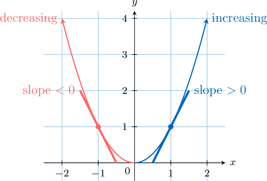
A function is increasing where the slope of its tangent is positive, and decreasing where the slope of its tangent is negative.
Proposition — Strict Sign of the Derivative and Monotonicity
For a function \(f\) that is differentiable on an interval \(I\): - If \(f'(x) > 0\) for all \(x \in I\), then \(f\) is strictly increasing on \(I\).
- If \(f'(x) < 0\) for all \(x \in I\), then \(f\) is strictly decreasing on \(I\).
Proposition — From the Variations to the Sign of the Derivative
Let \(f\) be a function differentiable on an interval \(I\). - If \(f\) is increasing on \(I\), then \(f'(x) \geq 0\) for all \(x \in I\).
- If \(f\) is decreasing on \(I\), then \(f'(x) \leq 0\) for all \(x \in I\).
- If \(f\) is constant on \(I\), then \(f'(x) = 0\) for all \(x \in I\).
Let \(a \in I\) and suppose that \(f\) is increasing on \(I\). For \(x \in I\) with \(x \neq a\), consider the rate of change \(\dfrac{f(x)-f(a)}{x-a}\).
If \(f\) is decreasing, the same reasoning gives a quotient less than or equal to \(0\), hence \(f'(a) \leq 0\). If \(f\) is constant, \(f(x) - f(a) = 0\): the rate of change is \(0\) and so is \(f'(a)\).
- If \(x < a\): since \(f\) is increasing, \(f(x) \leq f(a)\), so \(f(x) - f(a) \leq 0\) and \(x - a < 0\). The quotient of two numbers of the same sign is positive or zero.
- If \(x > a\): \(f(x) \geq f(a)\), so \(f(x) - f(a) \geq 0\) and \(x - a > 0\). Again the quotient is positive or zero.
If \(f\) is decreasing, the same reasoning gives a quotient less than or equal to \(0\), hence \(f'(a) \leq 0\). If \(f\) is constant, \(f(x) - f(a) = 0\): the rate of change is \(0\) and so is \(f'(a)\).
Proposition — Sign of the Derivative and Direction of Variation
The derivative may vanish at isolated points without changing the variations: if \(f'(x) \geq 0\) on \(I\), then \(f\) is increasing on \(I\), and if moreover \(f'\) vanishes only at a finite number of points, \(f\) is even strictly increasing. For instance \(f(x) = x^3\) has \(f'(x) = 3x^2 \geq 0\), which is zero only at \(x = 0\), and \(x^3\) is increasing on \(\mathbb{R}\). Together with the proposition “From the Variations to the Sign of the Derivative”: on an interval, \(f\) is increasing if and only if \(f' \geq 0\), and decreasing if and only if \(f' \leq 0\). Proposition — Characterisation of Constant Functions
Let \(f\) be a function differentiable on an interval \(I\). Then \(f\) is constant on \(I\) if and only if \(f'(x) = 0\) for all \(x \in I\). Method — Sign Diagram and Table of Variations
A sign diagram for the derivative, \(f'\), shows where the function is increasing or decreasing. This information is organised in a table of variations. Example
Find the variations of the function \(f(x)=x^2\).
The derivative of the function \(f(x)=x^2\) is \(f'(x)=2x\). 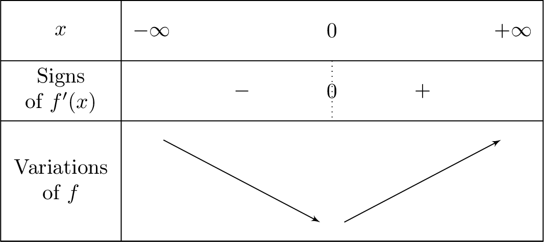
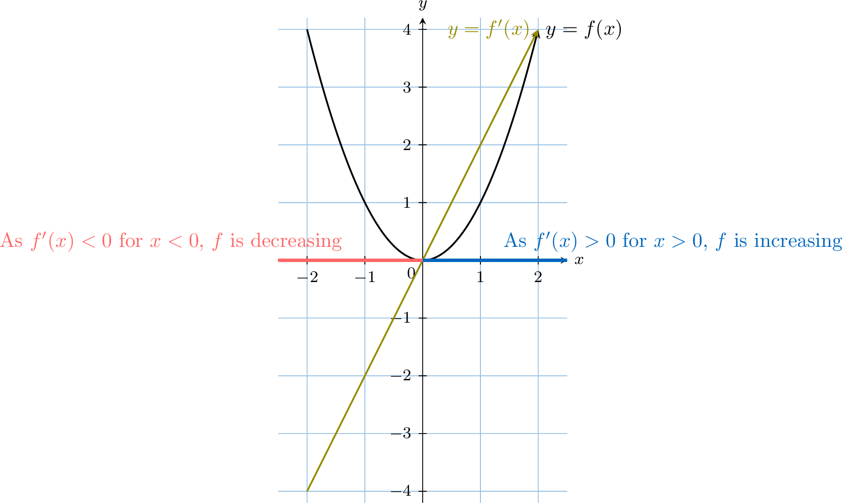
- The derivative \(f'(x)\) is negative on \((-\infty, 0)\), so the function \(f(x)\) is decreasing on \((-\infty, 0]\).
- The derivative \(f'(x)\) is positive on \((0,+\infty)\), so the function \(f(x)\) is increasing on \([0,+\infty)\).
Skills to practice
- Studying the Variations of a Function
III
Stationary Points and Extrema
III.1
Local and Global Extrema
Definition — Global Extrema
Let \(f\) be a function with domain \(D\). - \(f\) has a global maximum at \(x=c\) if \(f(c) \ge f(x)\) for all \(x\) in \(D\). The value \(f(c)\) is the maximum value of \(f\).
- \(f\) has a global minimum at \(x=c\) if \(f(c) \le f(x)\) for all \(x\) in \(D\). The value \(f(c)\) is the minimum value of \(f\).
Definition — Local Extrema
Let \(f\) be a function. - \(f\) has a local maximum at \(x=c\) if there is an open interval \(I\) containing \(c\) such that \(f(c) \ge f(x)\) for all \(x\) in \(I\).
- \(f\) has a local minimum at \(x=c\) if there is an open interval \(I\) containing \(c\) such that \(f(c) \le f(x)\) for all \(x\) in \(I\).
Definition — Stationary Point
A stationary point of a function \(f\) is a point \((c, f(c))\) on the curve where the tangent is horizontal, which means \(f^{\prime}(c)=0\). Proposition — Local Extrema and Stationary Points
Let \(f\) be a function defined on an open interval \(I\), and let \(c\in I\).If \(f\) has a local maximum or a local minimum at \(x=c\) and if \(f\) is differentiable at \(c\), then$$ f'(c)=0. $$
The condition \(f'(x_0) = 0\) is necessary for a local extremum at an interior point where \(f\) is differentiable, but it is not sufficient: for \(f(x) = x^3\), \(f'(0) = 0\) and yet \(f\) has no extremum at \(0\), since it keeps increasing. A function can also have an extremum at a point where it is not differentiable (\(|x|\) at \(0\)) or at an endpoint of its interval (\(x^2\) on \([1\,;\,3]\) has its minimum at \(1\) and its maximum at \(3\)): the proposition only concerns interior points where \(f\) is differentiable.
Proposition — First Derivative Test for Local Extrema
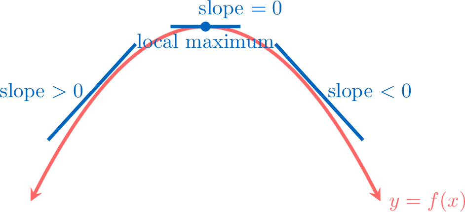
Let \(c\) be a number such that \(f'(c) = 0\). - If \(f^{\prime}(x)\) changes sign from positive to negative at \(x=c\), then \(f\) has a local maximum at \(c\).
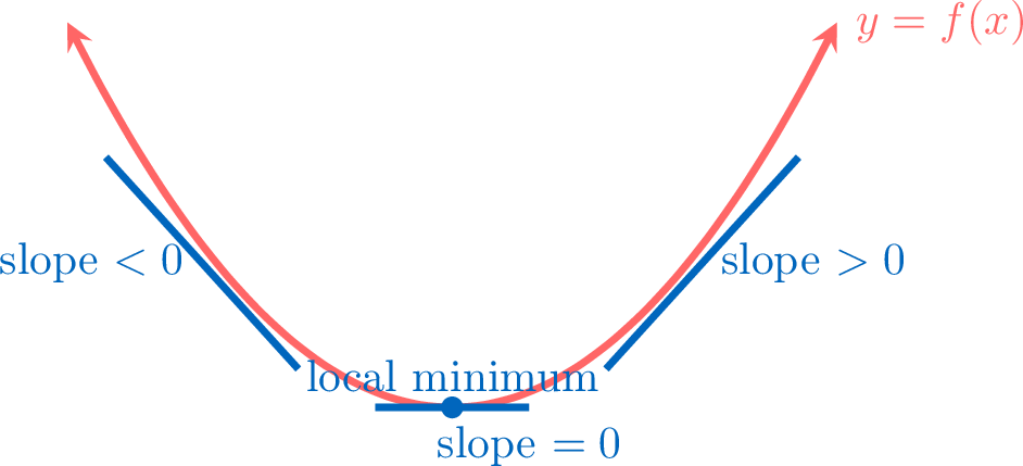
- If \(f^{\prime}(x)\) changes sign from negative to positive at \(x=c\), then \(f\) has a local minimum at \(c\).
Example
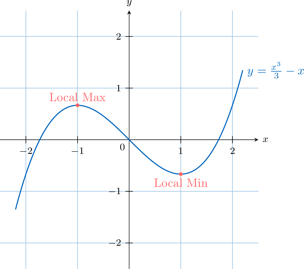
Find and classify the stationary points of \(f(x) = \frac{1}{3}x^3 - x\). - Find the derivative:$$ f'(x) = x^2 - 1. $$
- Find stationary points by solving \(f'(x)=0\):$$ \begin{aligned} x^2 - 1 &= 0 \\ (x-1)(x+1) &= 0.\end{aligned}$$ The stationary points are at \(x=-1\) and \(x=1\).
- Create the sign diagram for \(f'(x)\):
The derivative \(f'(x)=x^2-1\) is an upward-opening parabola with roots at \(-1\) and \(1\). It is positive outside the roots and negative between them. - Draw the table of variations and classify points:
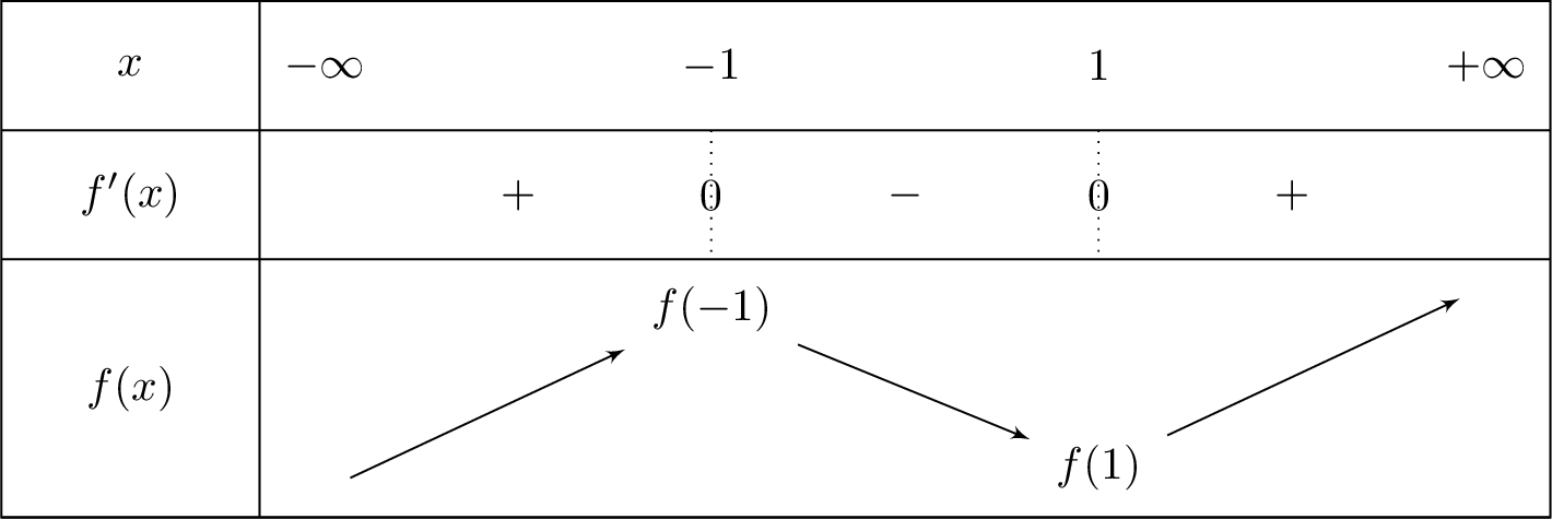
- At \(x=-1\), the sign of \(f'(x)\) changes from \(+\) to \(-\). Thus, there is a local maximum at \(x=-1\).$$f(-1) = \frac{1}{3}(-1)^3 - (-1) = \frac{2}{3}.$$
- At \(x=1\), the sign of \(f'(x)\) changes from \(-\) to \(+\). Thus, there is a local minimum at \(x=1\).$$f(1) = \frac{1}{3}(1)^3 - 1 = -\frac{2}{3}.$$
Proposition — The Quadratic Function Revisited
Let \(f(x) = ax^2 + bx + c\) with \(a \neq 0\). Then \(f\) is differentiable on \(\mathbb{R}\), \(f'(x) = 2ax + b\), and \(f'\) vanishes at \(x_0 = -\dfrac{b}{2a}\) while changing sign. - If \(a > 0\): \(f\) is decreasing on \((-\infty, x_0]\) and increasing on \([x_0, \infty)\); it has a minimum, equal to \(f(x_0)\), at \(x_0\).
- If \(a < 0\): \(f\) is increasing on \((-\infty, x_0]\) and decreasing on \([x_0, \infty)\); it has a maximum, equal to \(f(x_0)\), at \(x_0\).
\(f'(x) = 2ax + b\) is a linear function with gradient \(2a\); it vanishes at \(x_0 = -\dfrac{b}{2a}\). If \(a > 0\), then \(2a > 0\), so \(f'(x) < 0\) for \(x < x_0\) and \(f'(x) > 0\) for \(x > x_0\): \(f\) is decreasing then increasing, and \(f'\) vanishes at \(x_0\) while changing sign from \(-\) to \(+\), so \(f\) has a minimum at \(x_0\). If \(a < 0\), all the signs are reversed: \(f\) is increasing then decreasing, with a maximum at \(x_0\).
Skills to practice
- Finding and Classifying Stationary Points
III.2
Stationary Points with Technology
Method — Locating Stationary Points with the Graph of the Derivative
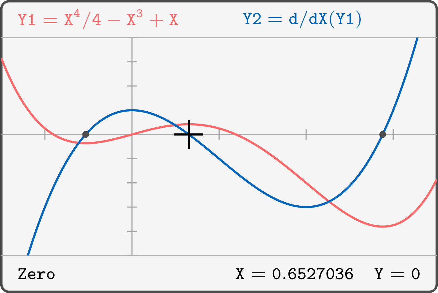
When the equation \(f'(x) = 0\) cannot be solved by hand, a graphing calculator locates the stationary points of \(f\) from the graph of \(f'\), which it generates from the expression of \(f\) alone: - Enter \(f(x)\) as \(Y_1\), then generate \(f'\) as \(Y_2\): the derivative command applied to \(Y_1\) at the point \(X\), written \(\frac{\mathrm{d}}{\mathrm{d}X}(Y_1)\big|_{X=X}\) on most models. When the expression of \(f'(x)\) is known, enter it instead.
- Solve \(f'(x) = 0\): the zero tool applied to \(Y_2\), with bounds on either side of each \(x\)-intercept, gives the \(x\)-coordinates of the stationary points of \(f\). Store each value. The zero tool looks for a change of sign, so it may miss a point where the graph of \(f'\) touches the axis without crossing it: such a point is a local maximum or minimum of \(f'\) of value \(0\), found with the maximum or minimum tool applied to \(Y_2\).
- Classify each stationary point with the sign of \(f'\) on either side, read on the graph of \(Y_2\): where it crosses the \(x\)-axis from above to below, \(f\) has a local maximum; from below to above, a local minimum; where it touches the axis without crossing, neither. These readings concern the isolated zeros of \(f'\), where the graph of \(Y_2\) meets the axis at a single point; where the graph of \(Y_2\) runs along the \(x\)-axis over a whole interval, \(f' = 0\) there and \(f\) is constant on that interval.
- Compute the \(y\)-coordinates with the value tool on \(Y_1\), at the stored \(x\)-coordinates, and report the coordinates to 3 significant figures.
The mock-up generates the graph of \(f'\) for \(f(x) = \dfrac{x^4}{4} - x^3 + x\), and the zero tool finds one of its three \(x\)-intercepts: the stationary points of \(f\) are at \(x \approx -0.532\), \(x \approx 0.653\) and \(x \approx 2.88\).
Example
Let \(f(x) = x^4 - 3x^3 + x + 2\), for \(-1 \le x \le 3\). - Use technology to generate the graph of \(f'\), and find the \(x\)-coordinates of the stationary points of \(f\), to 3 significant figures.
- Determine the nature of each stationary point, and its coordinates.
- Find the greatest value and the least value of \(f\) on \([-1, 3]\).
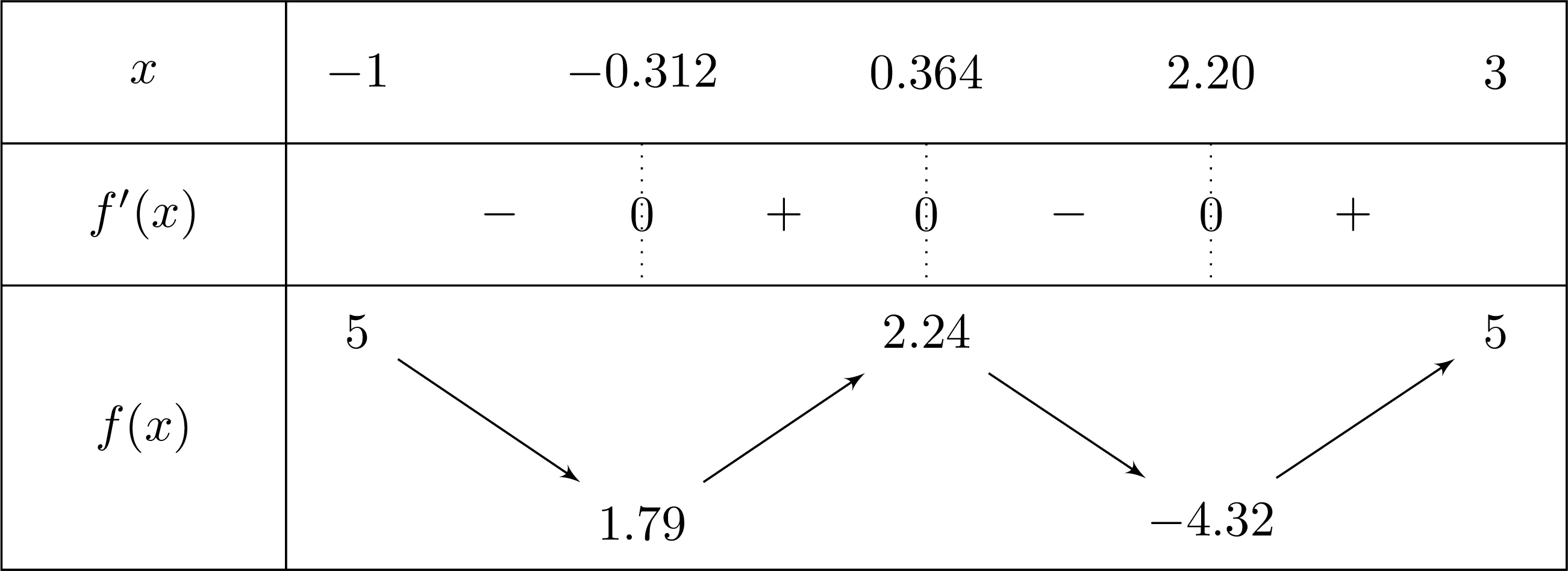
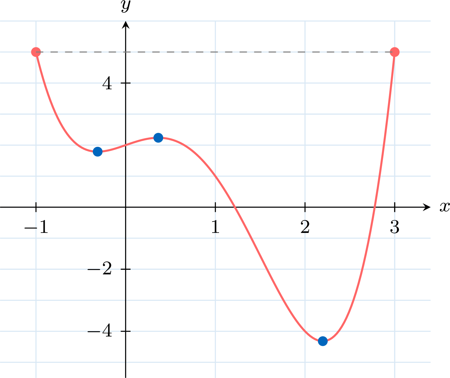
- \(f\) is a polynomial function, differentiable on \([-1, 3]\), and \(f'(x) = 4x^3 - 9x^2 + 1\): this equation of degree \(3\) has no integer or simple fractional root, so the calculator solves it. With \(Y_1 = X^4 - 3X^3 + X + 2\) and \(Y_2 = \frac{\mathrm{d}}{\mathrm{d}X}(Y_1)\big|_{X=X}\), in the window \(-1 \le x \le 3\), \(-6 \le y \le 6\), the graph of \(f'\) crosses the \(x\)-axis three times. The zero tool displays \(X = -0.3123563\), \(X = 0.3640907\) and \(X = 2.1982656\): the stationary points are at \(x \approx -0.312\), \(x \approx 0.364\) and \(x \approx 2.20\). The polynomial solver, applied to \(4x^3 - 9x^2 + 1 = 0\), returns the same three values.
- On the screen, the graph of \(f'\) is below the \(x\)-axis before \(-0.312\), above it between \(-0.312\) and \(0.364\), below it between \(0.364\) and \(2.20\), and above it after \(2.20\). By the first derivative test, \(f\) has a local minimum at \(x \approx -0.312\), a local maximum at \(x \approx 0.364\) and a local minimum at \(x \approx 2.20\). The value tool on \(Y_1\), at the stored \(x\)-coordinates, displays \(1.7885894\), \(2.2368696\) and \(-4.3184277\): the points are \((-0.312, 1.79)\), \((0.364, 2.24)\) and \((2.20, -4.32)\).
- At the endpoints, \(f(-1) = 1 + 3 - 1 + 2 = 5\) and \(f(3) = 81 - 81 + 3 + 2 = 5\). The table of variations gathers the values:
Skills to practice
- Locating Stationary Points with Technology
- Finding Global Extrema on an Interval
IV
Concavity
IV.1
Concave Up and Concave Down
We have seen that the first derivative, \(f'(x)\), gives the slope of the curve \(y=f(x)\) at any value of \(x\).
The second derivative, \(f''(x)\), tells us the rate of change of the slope. It therefore gives us information about the shape or curvature of the curve.
The second derivative, \(f''(x)\), tells us the rate of change of the slope. It therefore gives us information about the shape or curvature of the curve.
Definition — Concavity
A function \(f\) is: - concave up on an interval if its graph bends upwards, like a cup
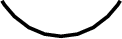 . The tangents lie below the curve.
- concave down on an interval if its graph bends downwards, like a cap
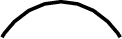 . The tangents lie above the curve.
Example
The curve \(f(x)=x^2\) is always concave up. The tangents lie below the curve. 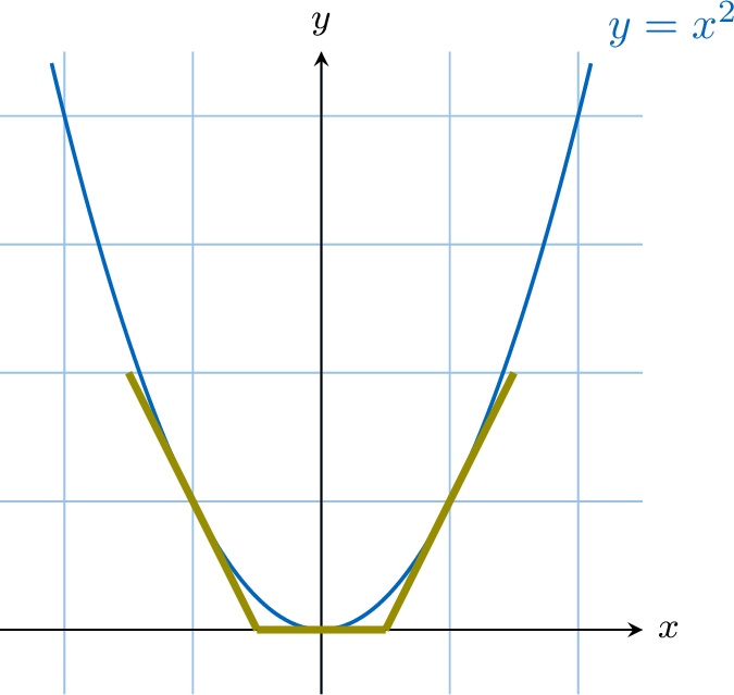
Skills to practice
- Concave Up and Concave Down
IV.2
Second Derivative Test for Concavity
Consider the curve below, which is concave down. 
As we move along the curve from left to right, \(x\) increases, but the slope of the tangent decreases (from \(2\), to \(1\), to \(0\), to \(-1\), etc.).
This means that the derivative function, \(f'\), is a decreasing function. If \(f'\) is decreasing, then its own derivative satisfies \(f''(x)\leq 0\) (where defined).
This means that the derivative function, \(f'\), is a decreasing function. If \(f'\) is decreasing, then its own derivative satisfies \(f''(x)\leq 0\) (where defined).
Proposition — Second Derivative Test for Concavity
For a function \(f\) that is twice differentiable on an interval \(I\): - \(f''(x) \ge 0\) for all \(x \in I\), if and only if \(f\) is concave up on \(I\).
- \(f''(x) \le 0\) for all \(x \in I\), if and only if \(f\) is concave down on \(I\).
Example
Show that \(f(x)=\ln(x)\) is concave down on its domain.
The domain of \(f(x)=\ln(x)\) is \((0,+\infty)\).
We find the first and second derivatives:$$ f'(x)=\frac 1 x \quad \text{and} \quad f''(x)=-\frac{1}{x^2}. $$ For all \(x\) in the domain, \(x^2 > 0\), which means \(-\dfrac{1}{x^2} < 0\).
Since \(f''(x) < 0\) for all \(x \in (0, +\infty)\), the function is concave down on its entire domain. 
We find the first and second derivatives:$$ f'(x)=\frac 1 x \quad \text{and} \quad f''(x)=-\frac{1}{x^2}. $$ For all \(x\) in the domain, \(x^2 > 0\), which means \(-\dfrac{1}{x^2} < 0\).
Since \(f''(x) < 0\) for all \(x \in (0, +\infty)\), the function is concave down on its entire domain.
Skills to practice
- Determining Concavity
IV.3
Second Derivative Test for Local Extrema
At a stationary point the tangent is horizontal. If \(f''\) is positive around the point, the curve is concave up there: it lies above its tangents, and in particular above this horizontal one, so the point is a local minimum. If \(f''\) is negative around the point, the curve is concave down and lies below the horizontal tangent: the point is a local maximum. In fact the sign of \(f''\) at the stationary point alone is enough to decide its nature, without the sign diagram of \(f'\): the second derivative test states it, and its proof does not need the sign of \(f''\) around the point. 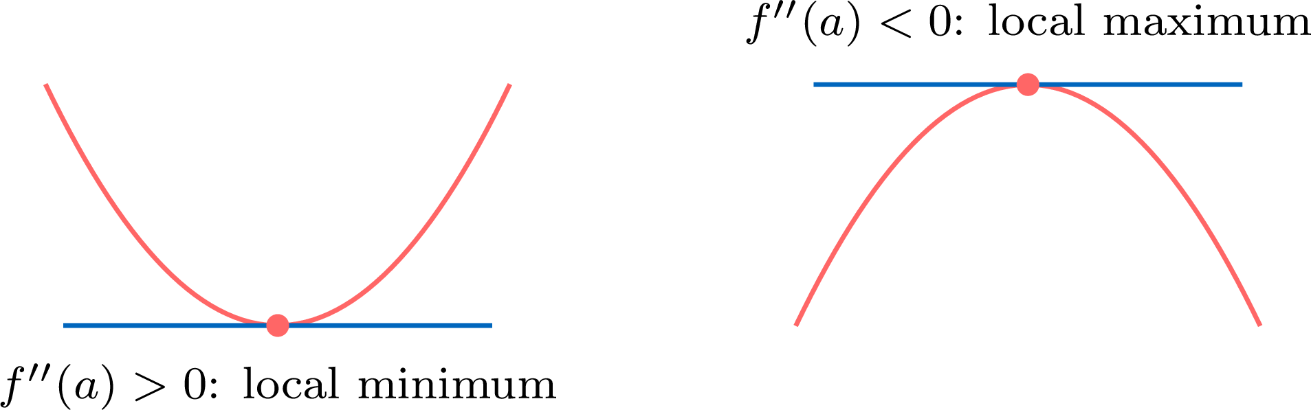
Proposition — Second Derivative Test for Local Extrema
Let \(f\) be a function twice differentiable on an open interval containing \(a\), with \(f'(a) = 0\). - If \(f''(a) > 0\), then \(f\) has a local minimum at \(a\).
- If \(f''(a) < 0\), then \(f\) has a local maximum at \(a\).
- If \(f''(a) = 0\), the test is inconclusive: \(f\) may have a local minimum, a local maximum or neither at \(a\), and another argument is needed, such as the sign of \(f'\) on either side of \(a\).
Suppose that \(f'(a) = 0\) and \(f''(a) > 0\). By definition, \(f''(a)\) is the derivative of \(f'\) at \(a\). Since \(f'(a) = 0\), for \(h \neq 0\), $$\frac{f'(a + h) - f'(a)}{h} = \frac{f'(a + h)}{h} \xrightarrow[h \to 0]{} f''(a).$$ This limit is positive, so the quotient \(\dfrac{f'(a + h)}{h}\) is positive for every \(h \neq 0\) close enough to \(0\): there is \(\delta > 0\) such that \(\dfrac{f'(a + h)}{h} > 0\) whenever \(0 < |h| < \delta\). A quotient is positive when its two terms have the same sign, so \(f'(a + h)\) has the sign of \(h\):
If \(f''(a) < 0\), the same reasoning with every inequality reversed shows that \(f'\) changes sign from positive to negative at \(a\): \(f\) has a local maximum at \(a\).
If \(f''(a) = 0\), no conclusion is possible. The functions \(x \mapsto x^4\), \(x \mapsto -x^4\) and \(x \mapsto x^3\) all satisfy \(f'(0) = 0\) and \(f''(0) = 0\). On one hand, \(x^4 \ge 0\) and \(-x^4 \le 0\) for every \(x\): the first has a local minimum at \(0\), the second a local maximum. On the other hand, \(x^3 < 0\) for \(x < 0\) and \(x^3 > 0\) for \(x > 0\): the third has no extremum at \(0\). Hence the three cases of the statement.
- for \(-\delta < h < 0\), \(f'(a + h) < 0\): \(f'\) is negative just to the left of \(a\);
- for \(0 < h < \delta\), \(f'(a + h) > 0\): \(f'\) is positive just to the right of \(a\).
If \(f''(a) < 0\), the same reasoning with every inequality reversed shows that \(f'\) changes sign from positive to negative at \(a\): \(f\) has a local maximum at \(a\).
If \(f''(a) = 0\), no conclusion is possible. The functions \(x \mapsto x^4\), \(x \mapsto -x^4\) and \(x \mapsto x^3\) all satisfy \(f'(0) = 0\) and \(f''(0) = 0\). On one hand, \(x^4 \ge 0\) and \(-x^4 \le 0\) for every \(x\): the first has a local minimum at \(0\), the second a local maximum. On the other hand, \(x^3 < 0\) for \(x < 0\) and \(x^3 > 0\) for \(x > 0\): the third has no extremum at \(0\). Hence the three cases of the statement.
Example
Find the stationary points of \(f(x) = x^3 - 6x^2 + 9x + 1\) and determine their nature with the second derivative test.
Stationary points. $$\begin{aligned}[t] f'(x) &= 3x^2 - 12x + 9 &&\text{(power rule)} \\
&= 3(x^2 - 4x + 3) &&\text{(common factor } 3\text{)} \\
&= 3(x - 1)(x - 3). &&\text{(factorise)} \end{aligned}$$ By the null factor law, \(f'(x) = 0\) for \(x = 1\) and \(x = 3\).
Second derivative. \(f''(x) = 6x - 12\). 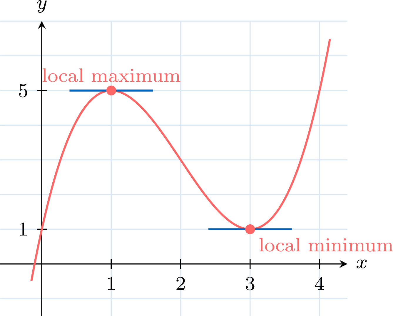
Second derivative. \(f''(x) = 6x - 12\).
- \(f''(1) = 6 - 12 = -6 < 0\): local maximum, with \(f(1) = 1 - 6 + 9 + 1 = 5\).
- \(f''(3) = 18 - 12 = 6 > 0\): local minimum, with \(f(3) = 27 - 54 + 27 + 1 = 1\).
Example
Let \(f(x) = x^4 - 4x^3\). Find the stationary points of \(f\) and determine their nature. Where the second derivative test does not conclude, use the sign of \(f'\).
Stationary points. $$\begin{aligned}[t] f'(x) &= 4x^3 - 12x^2 &&\text{(power rule)} \\
&= 4x^2(x - 3). &&\text{(common factor } 4x^2\text{)} \end{aligned}$$ So \(f'(x) = 0\) for \(x = 0\) and \(x = 3\), and \(f''(x) = 12x^2 - 24x = 12x(x - 2)\). 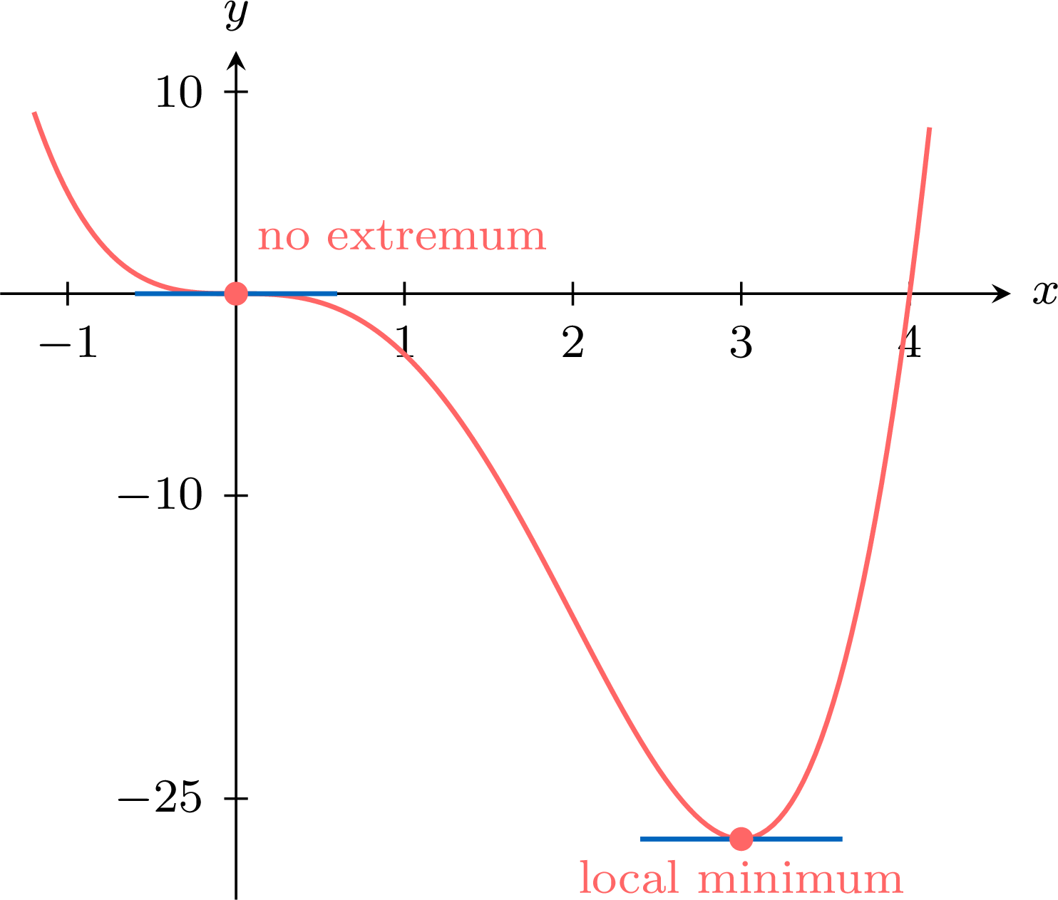
- At \(x = 3\): \(f''(3) = 12 \times 3 \times 1 = 36 > 0\), so \(f\) has a local minimum at \(3\), with \(f(3) = 81 - 108 = -27\).
- At \(x = 0\): \(f''(0) = 0\), and the test is inconclusive. The sign of \(f'(x) = 4x^2(x - 3)\) decides: \(4x^2 > 0\) for \(x \neq 0\), and \(x - 3 < 0\) for \(x < 3\), so \(f'(x) < 0\) on both sides of \(0\). The derivative does not change sign: \(f\) is decreasing through \((0, 0)\), which is not an extremum.
Skills to practice
- Reading the Second Derivative
- Written Practice: The Second Derivative Test
V
Points of Inflection
V.1
Definition of a Point of Inflection
A point of inflection marks a subtle but important change in the behavior of a function. While the function may still be increasing or decreasing, the rate at which it does so changes from accelerating to decelerating, or vice versa.
Consider the total number of cases during the start of an epidemic. Initially, the number of new cases per day increases, meaning the curve of total cases is steepening (concave up). At some point, measures are taken and the number of new cases per day, while still positive, starts to decrease. The curve of total cases begins to flatten (concave down). The moment this transition occurs is the point of inflection. It is the point where the rate of growth is at its maximum.
Consider the total number of cases during the start of an epidemic. Initially, the number of new cases per day increases, meaning the curve of total cases is steepening (concave up). At some point, measures are taken and the number of new cases per day, while still positive, starts to decrease. The curve of total cases begins to flatten (concave down). The moment this transition occurs is the point of inflection. It is the point where the rate of growth is at its maximum.
Definition — Point of Inflection
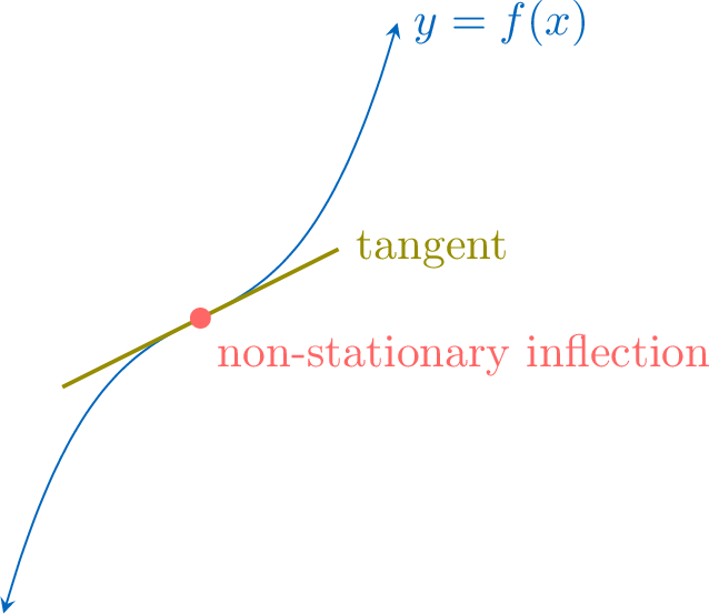
A point of inflection is a point on a curve where the concavity changes (from up to down, or from down to up). The tangent line crosses the curve at that point. 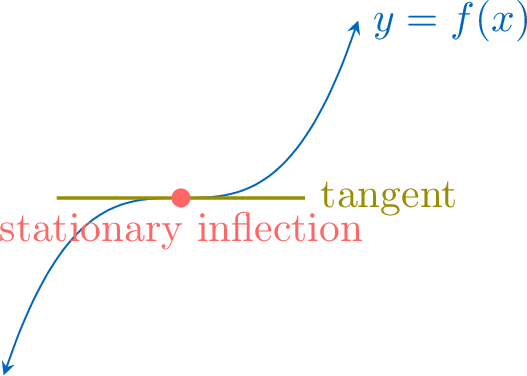 \(\quad\)
Skills to practice
- Definition of a Point of Inflection
V.2
Second Derivative Test for Points of Inflection
Since concavity is determined by the sign of the second derivative \(f''(x)\), a point of inflection must occur where \(f''(x)\) changes sign. For this to happen, \(f''\) must be zero at that point.
Proposition — Second Derivative Test for a Point of Inflection
A point \((a, f(a))\) is a point of inflection if \(f''(a)=0\) and the sign of \(f''(x)\) changes at \(x=a\).The point of inflection is:
- stationary if \(f'(a)=0\).
- non-stationary if \(f'(a) \neq 0\).
Example
For \(f(x)=x^3\), find and classify the point of inflection. - Find first and second derivatives:$$ f'(x) = 3x^2 $$ $$ f''(x) = 6x. $$
- Find potential inflection points by solving \(f''(x)=0\):$$ 6x = 0 \implies x=0. $$
- Check for sign change in \(f''(x)\) at \(x=0\):
- For \(x<0\), \(f''(x) = 6x < 0\) (concave down).
- For \(x>0\), \(f''(x) = 6x > 0\) (concave up).
- Classify the inflection point:
We check the value of the first derivative at \(x=0\):$$ f'(0) = 3(0)^2 = 0. $$ Since \(f'(0)=0\), the point \((0,0)\) is a stationary point of inflection.

Example
Let \(f(x) = x^4\). Show that \(f''(0) = 0\), and that the curve of \(f\) nevertheless has no point of inflection at the origin. Determine the nature of the point \((0, 0)\).
The second derivative. $$\begin{aligned}[t] f'(x) &= 4x^3, &&\text{(power rule)} \\
f''(x) &= 12x^2. &&\text{(power rule)} \end{aligned}$$ So \(f''(0) = 0\): the origin is only a candidate for a point of inflection.
The sign of \(f''\). For every \(x \neq 0\), \(x^2 > 0\), so \(f''(x) = 12x^2 > 0\): \(f''\) is positive on both sides of \(0\) and does not change sign there. Hence \(f''(x) \ge 0\) for every real \(x\), and by the second derivative test for concavity the curve is concave up on the whole real line. Its concavity never changes: \((0, 0)\) is not a point of inflection.
The nature of \((0, 0)\). \(f'(0) = 0\), and \(f'(x) = 4x^3\) is negative for \(x < 0\) and positive for \(x > 0\). By the first derivative test for local extrema, \((0, 0)\) is a local minimum; since \(x^4 \ge 0\) for every \(x\), it is even the least value of \(f\).
A zero of \(f''\) is only a candidate: a point of inflection requires \(f''\) to change sign, as the second derivative test for a point of inflection states. 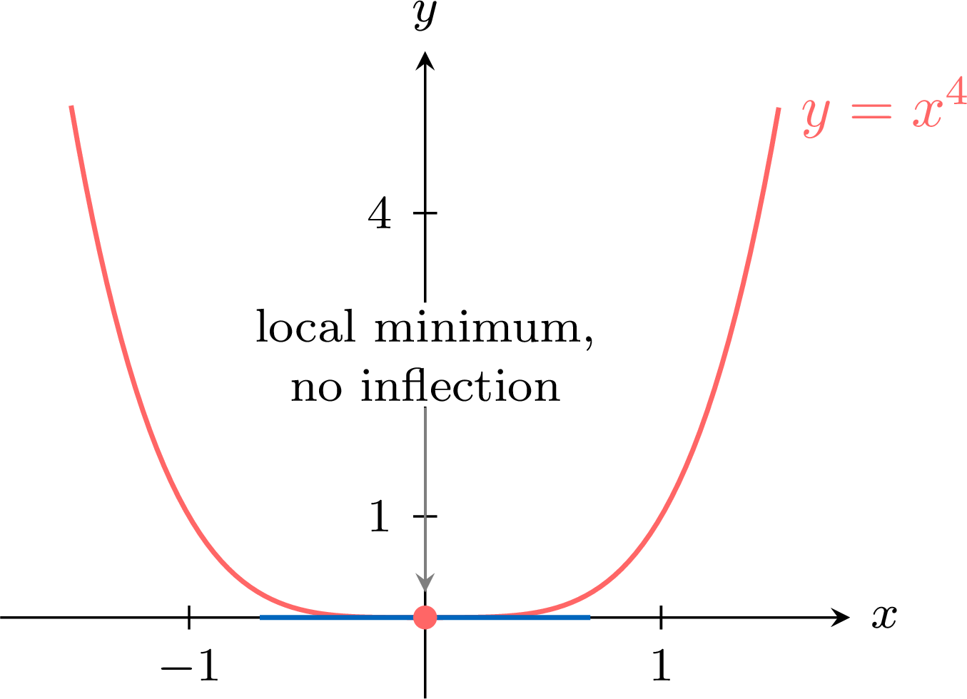
The sign of \(f''\). For every \(x \neq 0\), \(x^2 > 0\), so \(f''(x) = 12x^2 > 0\): \(f''\) is positive on both sides of \(0\) and does not change sign there. Hence \(f''(x) \ge 0\) for every real \(x\), and by the second derivative test for concavity the curve is concave up on the whole real line. Its concavity never changes: \((0, 0)\) is not a point of inflection.
The nature of \((0, 0)\). \(f'(0) = 0\), and \(f'(x) = 4x^3\) is negative for \(x < 0\) and positive for \(x > 0\). By the first derivative test for local extrema, \((0, 0)\) is a local minimum; since \(x^4 \ge 0\) for every \(x\), it is even the least value of \(f\).
A zero of \(f''\) is only a candidate: a point of inflection requires \(f''\) to change sign, as the second derivative test for a point of inflection states.
Example
Let \(f(x) = x^3 + 3x^2 - 9x + 2\). Find the point of inflection of the curve of \(f\), and state whether it is stationary or non-stationary.
The derivatives. \(f'(x) = 3x^2 + 6x - 9\) by the power rule, and $$\begin{aligned}[t] f''(x) &= 6x + 6 &&\text{(power rule, applied to } f'\text{)} \\
&= 6(x + 1). &&\text{(common factor } 6\text{)} \end{aligned}$$ The candidate. \(f''(x) = 0 \iff x = -1\).
The change of sign. \(6(x + 1)\) is negative for \(x < -1\) and positive for \(x > -1\): \(f''\) changes sign at \(-1\). The curve is concave down on \((-\infty, -1]\) and concave up on \([-1, +\infty)\), so by the second derivative test for a point of inflection it has a point of inflection at \(x = -1\), with $$f(-1) = -1 + 3 + 9 + 2 = 13.$$ Its nature. \(f'(-1) = 3 - 6 - 9 = -12 \neq 0\): the tangent at \((-1, 13)\) is not horizontal, and \((-1, 13)\) is a non-stationary point of inflection.
The gradient also shows why the point is special: \(f'(x) = 3(x + 1)^2 - 12\) is least at \(x = -1\). At the point of inflection the curve falls most steeply, with gradient \(-12\); it rises to its local maximum \((-3, 29)\) before, and down to its local minimum \((1, -3)\) after. 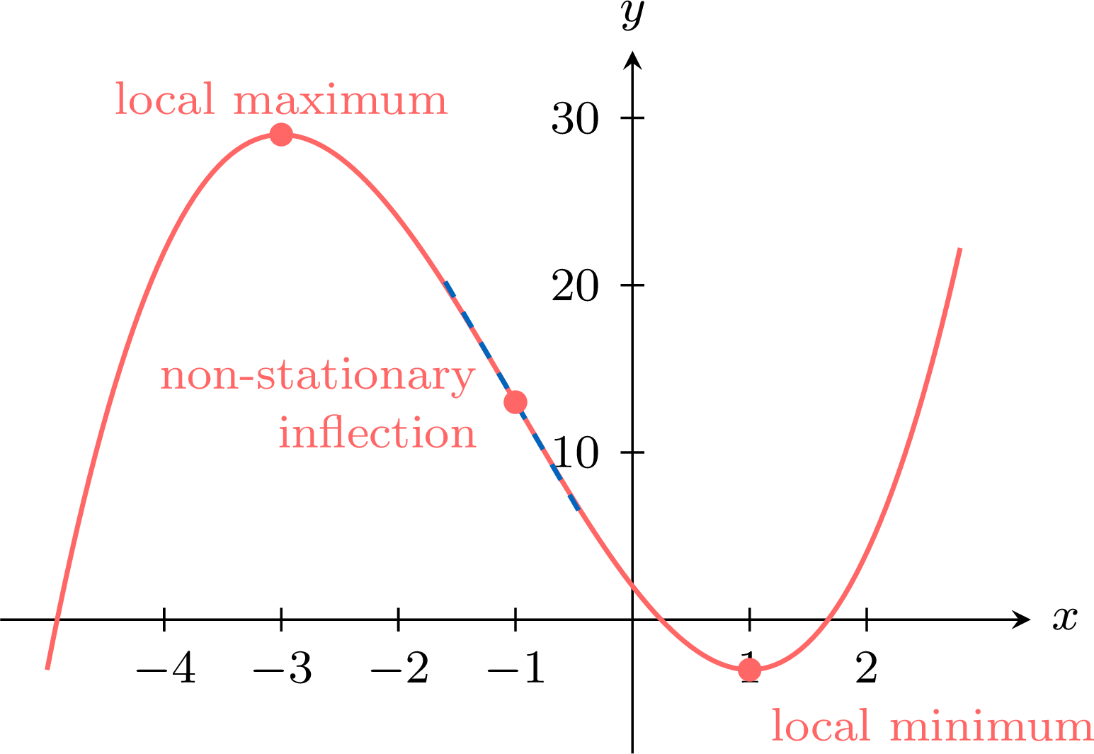
The change of sign. \(6(x + 1)\) is negative for \(x < -1\) and positive for \(x > -1\): \(f''\) changes sign at \(-1\). The curve is concave down on \((-\infty, -1]\) and concave up on \([-1, +\infty)\), so by the second derivative test for a point of inflection it has a point of inflection at \(x = -1\), with $$f(-1) = -1 + 3 + 9 + 2 = 13.$$ Its nature. \(f'(-1) = 3 - 6 - 9 = -12 \neq 0\): the tangent at \((-1, 13)\) is not horizontal, and \((-1, 13)\) is a non-stationary point of inflection.
The gradient also shows why the point is special: \(f'(x) = 3(x + 1)^2 - 12\) is least at \(x = -1\). At the point of inflection the curve falls most steeply, with gradient \(-12\); it rises to its local maximum \((-3, 29)\) before, and down to its local minimum \((1, -3)\) after.
Skills to practice
- Locating and Classifying Points of Inflection
- Determining Points of Inflection
VI
Graphs of \(f\), \(f'\) and \(f''\)
VI.1
Reading \(f\) from the Graph of \(f'\)
The graphs of \(f\), \(f'\) and \(f''\) describe one function at three levels: the curve of \(f\) gives its values, the graph of \(f'\) the slope of that curve at each point, and the graph of \(f''\) the way this slope changes. The direction of variation of \(f\) is read on the sign of \(f'\), its concavity on the sign of \(f''\): where the graph of \(f'\) lies above the \(x\)-axis, the curve of \(f\) rises; where the graph of \(f''\) lies above it, the curve of \(f\) is concave up. The position of the curve of \(f\), however, cannot be read on the graph of \(f'\): \(f\) and \(f + 5\) have the same derivative.
Method — Reading the Variations and Extrema of \(f\) from the Graph of \(f'\)
To read the behaviour of a function \(f\), twice differentiable on an interval, from the graph of its derivative \(f'\): - Variations: where the graph of \(f'\) lies above the \(x\)-axis, \(f\) is increasing; where it lies below, \(f\) is decreasing.
- Stationary points: each \(x\)-intercept of the graph of \(f'\) is the abscissa of a stationary point of \(f\). Where the graph of \(f'\) crosses the axis from above to below, \(f\) has a local maximum; from below to above, a local minimum; where it touches the axis at an isolated point without crossing, \(f\) has no extremum.
- Concavity: \(f''\) is the derivative of \(f'\). Where \(f'\) is increasing, \(f'' \ge 0\) and \(f\) is concave up; where \(f'\) is decreasing, \(f'' \le 0\) and \(f\) is concave down.
- Points of inflection: where \(f'\) changes from increasing to decreasing, or the reverse, the concavity of \(f\) changes: \(f\) has a point of inflection there, and the graph of \(f'\) has a local maximum or minimum.
Example
The graph below is the graph of the derivative \(f'\) of a function \(f\) defined on \(\mathbb{R}\); it is a parabola. 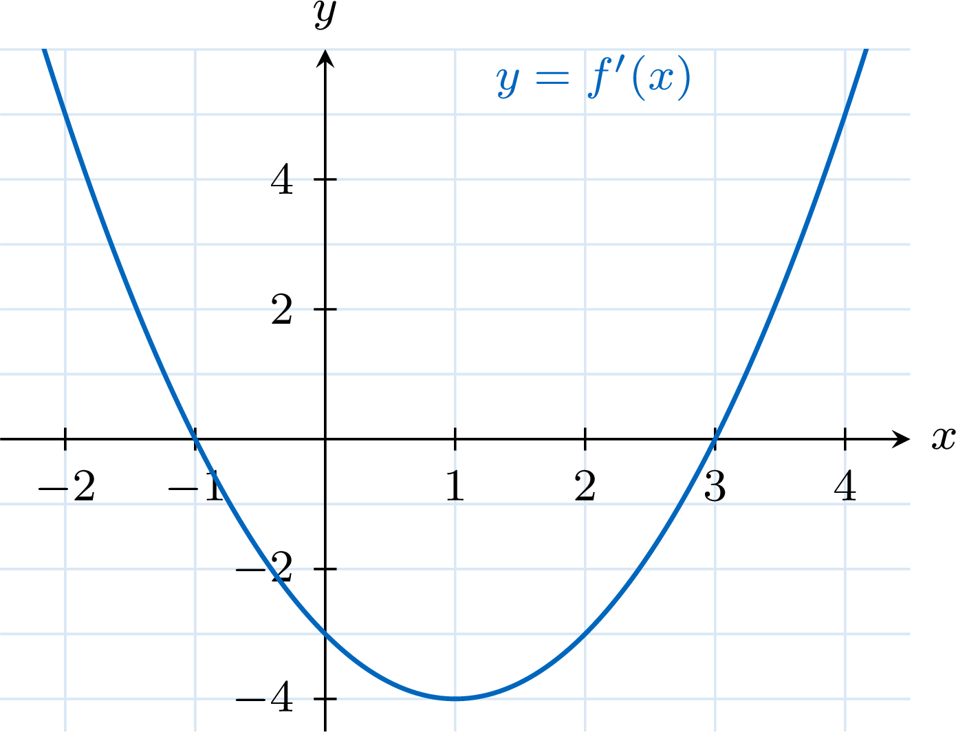
- Give the intervals on which \(f\) is increasing or decreasing, and the abscissas of its local extrema.
- Give the intervals on which \(f\) is concave up or concave down, and the abscissa of its point of inflection.
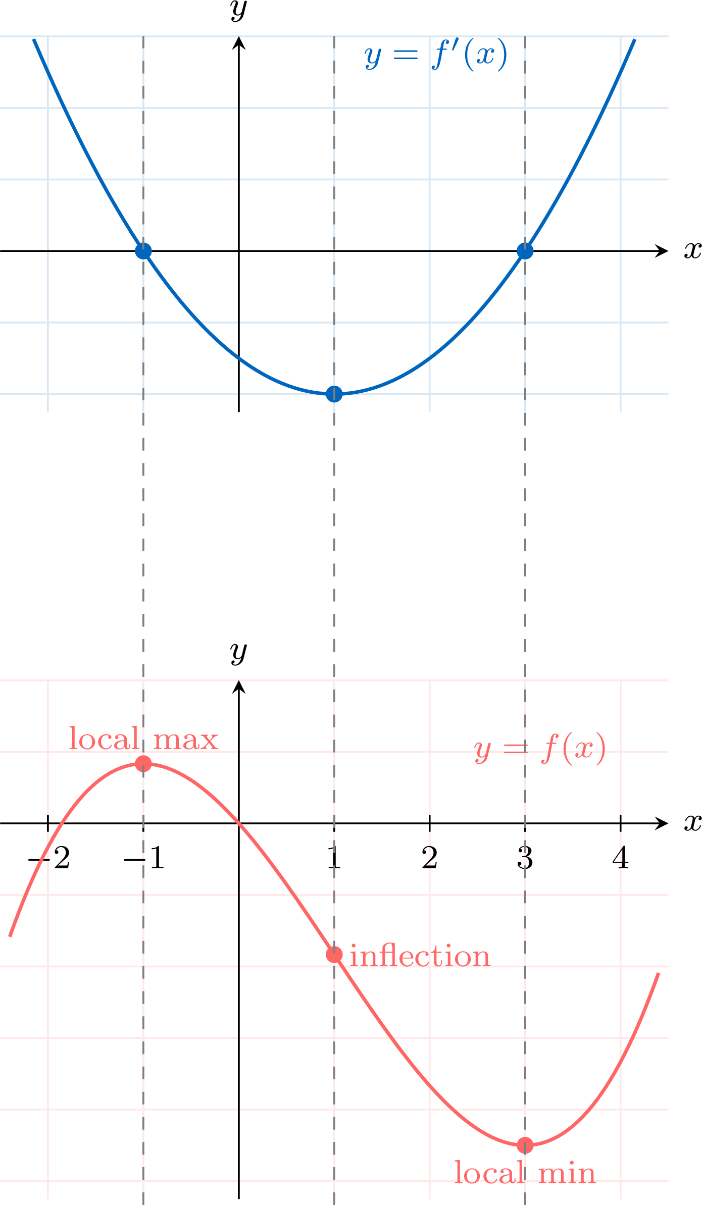
- Sketch a possible curve of \(f\), given that \(f(0) = 0\).
- The graph of \(f'\) is above the \(x\)-axis for \(x < -1\) and for \(x > 3\), and below it for \(-1 < x < 3\). So \(f\) is increasing on \((-\infty, -1]\) and on \([3, +\infty)\), and decreasing on \([-1, 3]\). The graph of \(f'\) crosses the axis from above to below at \(x = -1\): \(f\) has a local maximum at \(-1\); from below to above at \(x = 3\): a local minimum at \(3\).
- The graph of \(f'\) is a parabola with its lowest point at \(x = 1\): \(f'\) is decreasing on \((-\infty, 1]\) and increasing on \([1, +\infty)\). So \(f\) is concave down on \((-\infty, 1]\) and concave up on \([1, +\infty)\), and the curve of \(f\) has a point of inflection at \(x = 1\).
- The curve rises to a local maximum at \(x = -1\), falls through the point of inflection at \(x = 1\) to a local minimum at \(x = 3\), then rises again, and passes through the origin. One such function is \(f(x) = \dfrac{x^3}{3} - x^2 - 3x\): its derivative is \(x^2 - 2x - 3\), the parabola of the figure, and \(f(0) = 0\).
Skills to practice
- Interpreting the Graph of the Derivative
VI.2
Sketching \(f'\) and \(f''\) from the Graph of \(f\)
Method — Sketching the Graph of \(f'\) from the Curve of \(f\)
To sketch the graph of \(f'\) from the curve of a function \(f\) twice differentiable on an interval: - Mark the stationary points of \(f\): their abscissas are the \(x\)-intercepts of the graph of \(f'\).
- Place the graph of \(f'\) above or below the \(x\)-axis: on or above the axis on each interval where \(f\) is increasing, on or below it where \(f\) is decreasing; it meets the axis only at the abscissas of the horizontal tangents.
- Follow the steepness: the steeper the curve of \(f\), the farther the graph of \(f'\) from the \(x\)-axis. At a point of inflection of \(f\), the slope is locally the greatest or the least: the graph of \(f'\) has a local maximum or minimum there.
- Repeat with \(f'\) in place of \(f\) to sketch the graph of \(f''\): its \(x\)-intercepts are the abscissas of the stationary points of \(f'\), among them the points of inflection of \(f\).
Example
The curve of the function \(f(x) = -x^3 + 3x\) is shown below. 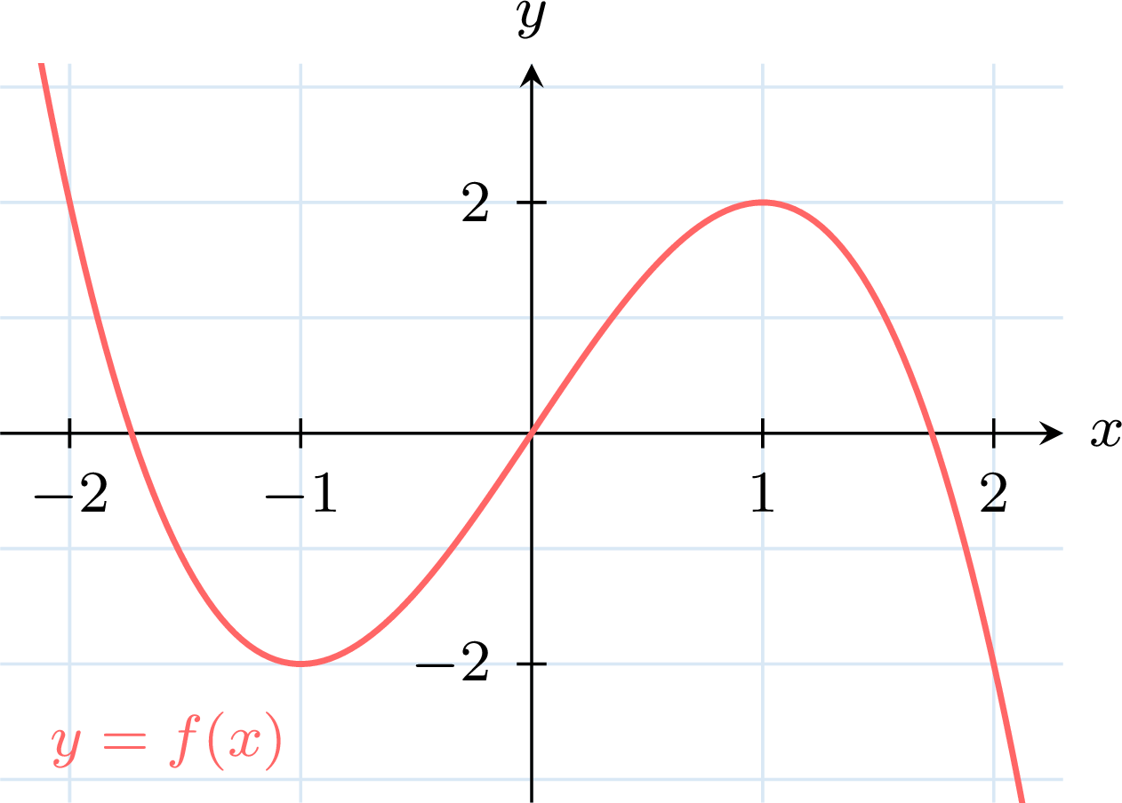
The graph of \(f'\). The curve of \(f\) has a local minimum at \(x = -1\) and a local maximum at \(x = 1\): the graph of \(f'\) crosses the \(x\)-axis at \(-1\) and \(1\). The curve falls on \((-\infty, -1]\), rises on \([-1, 1]\) and falls on \([1, +\infty)\): the graph of \(f'\) is below the axis, then above, then below. The curve is steepest while rising at its point of inflection, at \(x = 0\): the graph of \(f'\) has its highest point there.
The graph of \(f''\). The graph of \(f'\) rises until \(x = 0\), then falls: \(f''\) is positive before \(0\) and negative after, and its graph crosses the axis at \(0\), the abscissa of the point of inflection of \(f\). 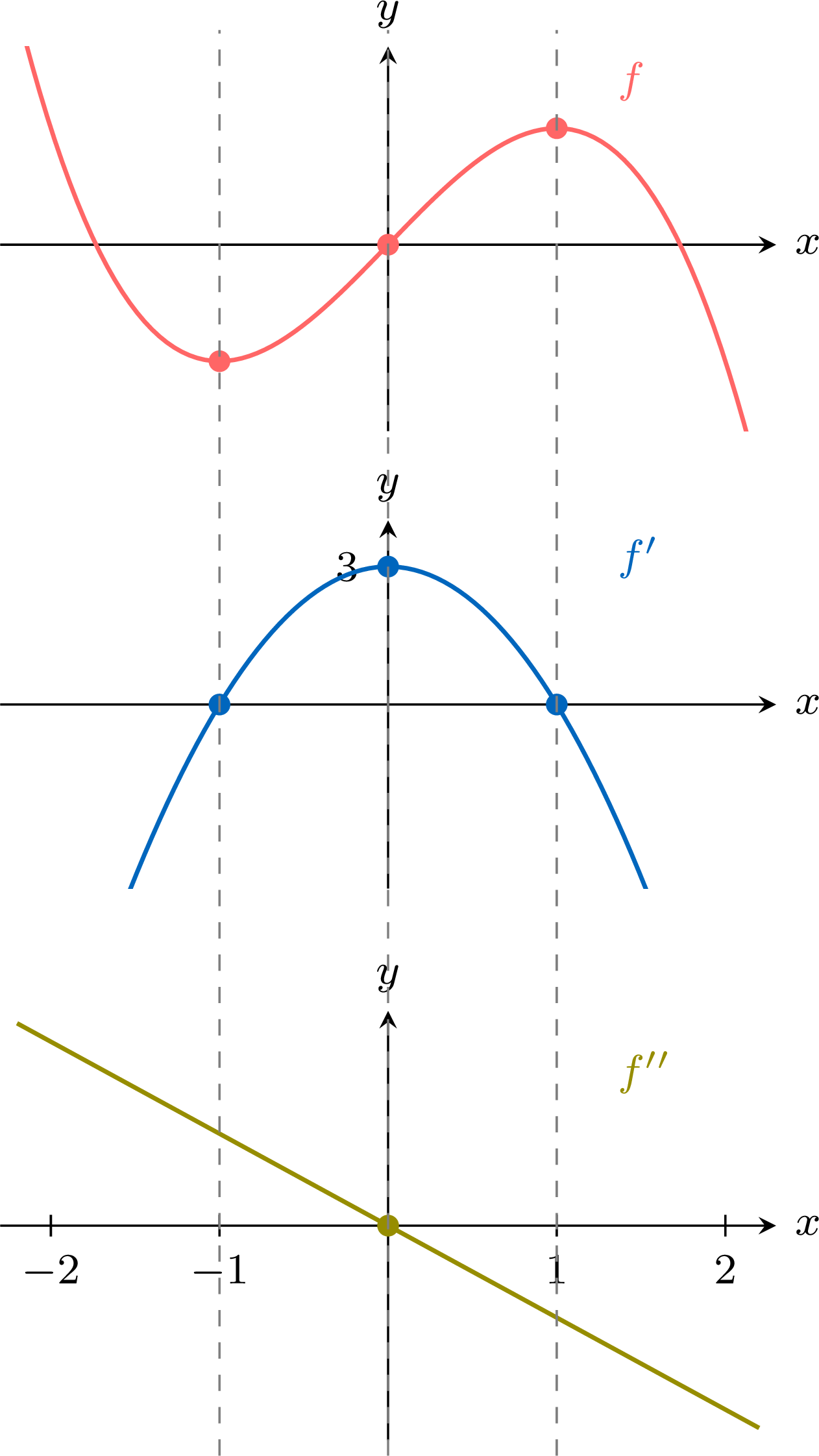
Check. \(f'(x) = -3x^2 + 3 = 3(1 - x^2)\), which vanishes at \(-1\) and \(1\) and is greatest, equal to \(3\), at \(0\); \(f''(x) = -6x\), positive for \(x < 0\), zero at \(0\), negative for \(x > 0\). The sketches have the right shape; the expressions add the exact values and the nature of the curves: a parabola for \(f'\), a line for \(f''\).
The graph of \(f''\). The graph of \(f'\) rises until \(x = 0\), then falls: \(f''\) is positive before \(0\) and negative after, and its graph crosses the axis at \(0\), the abscissa of the point of inflection of \(f\).
Skills to practice
- Matching the Graphs of \(f\) and \(f'\)
- Sketching the Graph of \(f'\) from the Curve of \(f\)
VI.3
Sketching a Curve
Method — Sketching the Shape of a Curve
To sketch the curve of a function \(f\) from what the derivatives say, using only what the derivatives have already given: - Frame: state the interval of study, then the limits of \(f\) at its endpoints. They tell where the curve escapes and where it stops, and they give the vertical asymptotes, at a finite endpoint where the limit is infinite, and the horizontal ones, at an infinite endpoint where the limit is finite. An oblique asymptote is not read off them and needs a comparison of its own.
- Variations: read the sign of \(f'\), build the table of variations of \(f\), and place the points where \(f'\) vanishes. Each of them is a horizontal tangent.
- Bending: read the sign of \(f''\), deduce the intervals where \(f\) is convex and those where it is concave, and place the points of inflection, where that sign changes at a point of the interval. A change of sign across a value where \(f\) is not defined gives none: \(x \mapsto 1/x\) has second derivatives of opposite signs on either side of \(0\) without any point of inflection.
- Drawing: put the notable points on the frame, respect the direction of variation on each interval, then bend each arc according to step 3: hollow upwards where \(f\) is convex, hollow downwards where \(f\) is concave.
Example
Sketch the curve of the function \(f\) defined on \(\mathbb{R}\) by \(f(x) = x^3 - 3x^2 + 3x\), following the four steps.
Frame. \(f\) is a polynomial, twice differentiable on \(\mathbb{R}\), and $$\lim_{x \to -\infty} f(x) = -\infty \qquad \text{and} \qquad \lim_{x \to +\infty} f(x) = +\infty.$$ The curve escapes downwards on the left and upwards on the right. And since \(\dfrac{f(x)}{x} = x^2 - 3x + 3\) grows beyond every bound at both ends, no line can stay close to the curve at infinity: there is no asymptote, oblique or otherwise, and none vertical either since \(f\) is continuous on all of \(\mathbb{R}\). Variations. Differentiating twice: $$\begin{aligned} f'(x) &= 3x^2 - 6x + 3 = 3(x-1)^2 && \text{(factorise)} \\
f''(x) &= 6x - 6 = 6(x-1) && \text{(differentiate again)} \end{aligned}$$ A square is never negative, so \(f'(x) \ge 0\) for every \(x\): \(f\) is increasing on the whole of \(\mathbb{R}\). Its derivative vanishes at \(x = 1\) alone, where \(f(1) = 1\); the tangent is horizontal there, but the sign of \(f'\) does not change, so this is not an extremum. 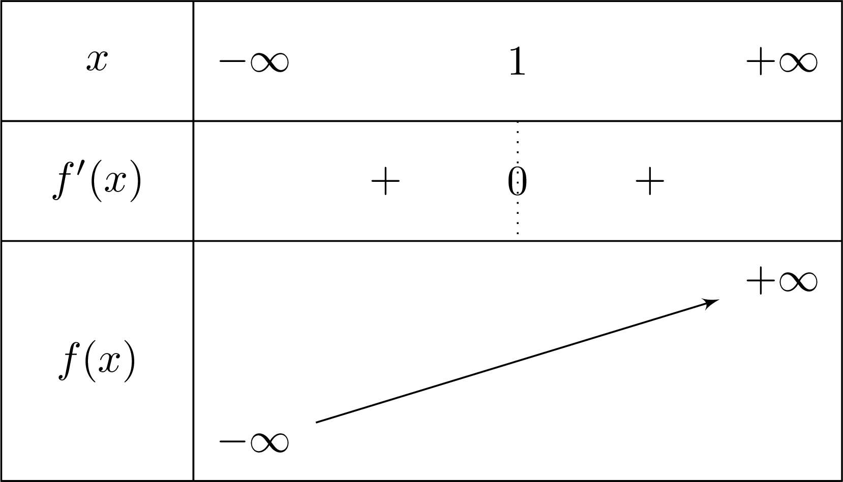
Bending. \(f''(x) = 6(x-1)\) is negative before \(1\) and positive after, and vanishes at \(1\) while changing sign: \(f\) is concave on \(]-\infty\,;\,1]\), convex on \([1\,;\,+\infty[\), and the point \((1\,;\,1)\) is a point of inflection. 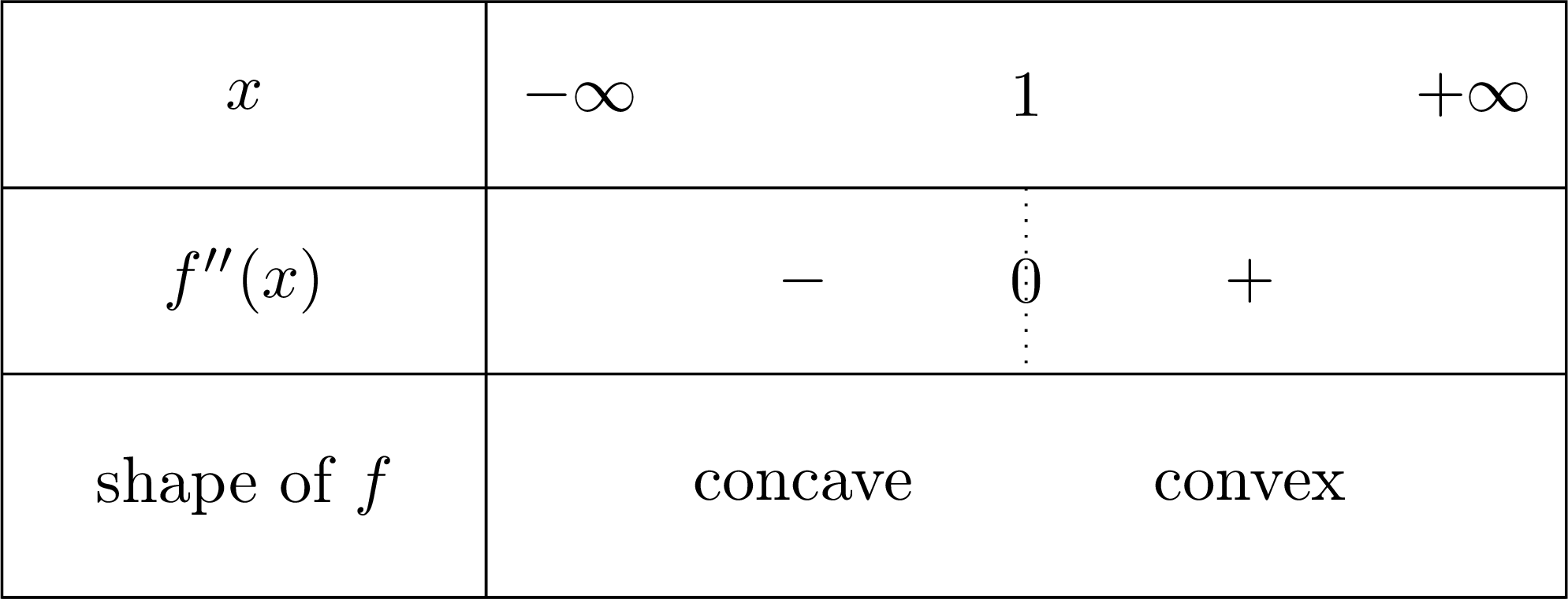
Drawing. One rising branch. Before \(1\) the curve stays below its tangents, after \(1\) above them; at \((1\,;\,1)\) it crosses the horizontal tangent \(y = 1\), which is what a point of inflection does. 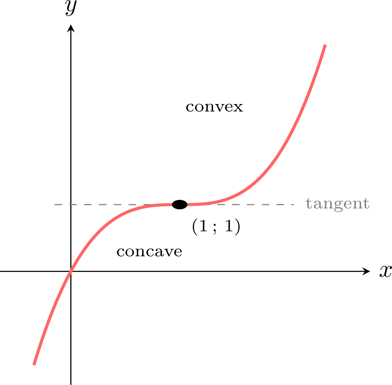
The curve rises everywhere, and yet it does not bend the same way on the two sides of \((1\,;\,1)\): step 3 sees what step 2 cannot.
Skills to practice
- Sketching the Shape of a Curve
VII
Limits of Indeterminate Forms
VII.1
L'Hôpital's Rule
The easiest way to evaluate a limit is direct substitution. However, this method sometimes produces an indeterminate form, such as \(\dfrac{0}{0}\) or \(\dfrac{\infty}{\infty}\). These forms do not have a defined value, but the limit might still exist.
For example, \(\displaystyle\lim_{x \to 0} \dfrac{e^x-1}{x}\) gives \(\dfrac{0}{0}\). L'Hôpital's Rule provides a powerful technique to solve limits of these specific indeterminate forms by using derivatives.
For example, \(\displaystyle\lim_{x \to 0} \dfrac{e^x-1}{x}\) gives \(\dfrac{0}{0}\). L'Hôpital's Rule provides a powerful technique to solve limits of these specific indeterminate forms by using derivatives.
Proposition — L'Hôpital's Rule
Suppose \(f\) and \(g\) are differentiable functions and \(g'(x)\neq 0\) on an open interval \(I\) containing \(a\) (except possibly at \(a\) itself). - Indeterminate Form \(\dfrac{0}{0}\):
If \(\displaystyle\lim_{x \to a} f(x) = 0\), \(\displaystyle\lim_{x \to a} g(x) = 0\) and \(\lim_{x \to a} \dfrac{f'(x)}{g'(x)}\) exists, then $$ \lim_{x \to a} \dfrac{f(x)}{g(x)} = \lim_{x \to a} \dfrac{f'(x)}{g'(x)} $$ - Indeterminate Form \(\dfrac{\infty}{\infty}\):
If \(\displaystyle\lim_{x \to a} f(x) = \pm\infty\), \(\displaystyle\lim_{x \to a} g(x) = \pm\infty\) and \(\lim_{x \to a} \dfrac{f'(x)}{g'(x)}\) exists, then $$ \lim_{x \to a} \dfrac{f(x)}{g(x)} = \lim_{x \to a} \dfrac{f'(x)}{g'(x)} $$
Example
Evaluate the limit \(\displaystyle\lim_{x \to 0} \dfrac{e^{x}-1}{x}\).
First, we check the form of the limit by direct substitution:$$ \lim_{x \to 0}(e^{x}-1) = e^0-1=0 \quad \text{and} \quad \lim_{x \to 0}(x) = 0 $$ This is the indeterminate form \(\dfrac{0}{0}\), so we can consider using L'Hôpital's Rule. We now find the limit of the ratio of the derivatives.$$\begin{aligned} \dfrac{\frac{d}{\mathrm{d}x}(e^x-1)}{\frac{d}{\mathrm{d}x}(x)} &= \dfrac{e^x}{1} \\
&\xrightarrow[x \to 0]{} \dfrac{e^0}{1} = 1\end{aligned}$$ Since the limit of the derivatives exists and is equal to 1, by L'Hôpital's Rule we can conclude:$$ \lim_{x \to 0} \dfrac{e^{x}-1}{x} = 1 $$ This limit is used elsewhere to establish \((e^x)' = e^x\): finding it again with L'Hôpital's Rule is a check, not a proof.
Skills to practice
- Applying L'Hôpital's Rule
VIII
Going further
Skills to practice
- Diagnosing and Correcting Errors
- Solving Problems
- Quiz
Jump to section