International Baccalaureate · DP 2: Analysis and Approaches HL

Maclaurin Series

⌚ ~170 min ▢ 19 blocks ✓ 91 exercises ➣ Prerequisites : Rules of Differentiation, Properties of Curves, Techniques of Integration

I The Binomial Theorem for Rational Exponents

I.1 The Binomial Theorem

Recappreviously studied — click to reread

Proposition — Binomial Theorem

For any non-negative integer $n$ and any real numbers $a$ and $b$, we have$$\begin{aligned}(a+b)^n&=\sum_{k=0}^{n} \binom{n}{k}a^{\,n-k}b^{\,k}\\ &= \binom{n}{0}a^n b^0 + \binom{n}{1}a^{n-1}b^1 + \binom{n}{2}a^{n-2}b^2 + \dotsb + \binom{n}{n}a^0 b^n\end{aligned}$$

Proof

Combinatorial Argument:
- Case $n=0$: By convention, $(a+b)^0 = 1$. The formula gives $\binom{0}{0}a^0b^0 = 1 \times 1 \times 1 = 1$. Thus, the theorem holds.
- Case $n > 0$: Consider the product$$(a+b)^n = \underbrace{(a+b)(a+b)\dotsm(a+b)}_{\text{$n$ factors}}.$$ To obtain a term in the expansion, we choose either $a$ or $b$ from each factor and multiply the $n$ choices together.
  A term of the form $a^{n-k}b^k$ appears whenever we choose $b$ from exactly $k$ of the $n$ brackets (and $a$ from the remaining $n-k$ brackets).
  The number of such choices is precisely $\binom{n}{k}$, because we must choose which $k$ positions will contribute a factor $b$.
  Therefore the coefficient of $a^{n-k}b^k$ is $\binom{n}{k}$, and summing over all $k$ from $0$ to $n$ gives$$(a+b)^n = \sum_{k=0}^{n} \binom{n}{k}a^{\,n-k}b^{\,k}.$$
Summing all possible terms from $k=0$ to $k=n$ gives the result.
Proof by Induction:
Let $P(n)$ be the property: $(a+b)^n = \sum_{k=0}^{n} \binom{n}{k} a^{n-k} b^k$.
- Base case: For $n=0$, $(a+b)^0 = 1$.
  The formula gives $\sum_{k=0}^{0} \binom{0}{k} a^{0-k} b^k = \binom{0}{0} a^0 b^0 = 1$.
  Thus $P(0)$ is true.
- Inductive step: Assume $P(n)$ is true for some $n \ge 0$. Let's compute $(a+b)^{n+1}$: $$(a+b)^{n+1} = (a+b) \sum_{k=0}^{n} \binom{n}{k} a^{n-k} b^k = \sum_{k=0}^{n} \binom{n}{k} a^{n-k+1} b^k + \sum_{k=0}^{n} \binom{n}{k} a^{n-k} b^{k+1}$$ By shifting the index of the second sum (let $j = k+1$), we combine the terms: $$(a+b)^{n+1} = \binom{n}{0}a^{n+1} + \sum_{k=1}^{n} \left[ \binom{n}{k} + \binom{n}{k-1} \right] a^{n-k+1} b^k + \binom{n}{n}b^{n+1}$$ Using Pascal's Identity, $\binom{n}{k} + \binom{n}{k-1} = \binom{n+1}{k}$, and noting that $\binom{n}{0}=\binom{n+1}{0}$ and $\binom{n}{n}=\binom{n+1}{n+1}$: $$(a+b)^{n+1} = \sum_{k=0}^{n+1} \binom{n+1}{k} a^{n+1-k} b^k.$$
Thus $P(n+1)$ is true, and the theorem is proven for all $n \in \mathbb{N}$.

Skills to practice

The Binomial Theorem

I.2 Rational Exponents

From a Finite Sum to an Infinite Series

For a non-negative integer $n$, the expansion of $(1+x)^n$ stops after $n+1$ terms. The exponent $n = -1$ already asks for more. For $|x| < 1$, $\dfrac{1}{1+x}$ is the sum of the infinite geometric series with first term $1$ and ratio $-x$: $$(1+x)^{-1} = 1 - x + x^2 - x^3 + \dotsb \qquad \text{for } |x| < 1.$$ Its coefficients $1, -1, 1, -1, \dots$ are exactly the numbers $\dfrac{n(n-1)\cdots(n-k+1)}{k!}$ computed with $n = -1$: for instance $\dfrac{(-1)(-2)}{2!} = 1$ and $\dfrac{(-1)(-2)(-3)}{3!} = -1$. Newton extended the binomial theorem in this way to every rational exponent. When the exponent is not a non-negative integer, there is a double price: the expansion becomes an infinite series, and it is valid only for some values of $x$.

Report an error

Definition — Binomial Coefficient for a Rational Exponent

Let $n$ be a rational number. For every integer $k \geq 1$, the binomial coefficient $\dbinom{n}{k}$ is $$\binom{n}{k} = \frac{n(n-1)(n-2)\cdots(n-k+1)}{k!},$$ a product of $k$ factors divided by $k!$, and $\dbinom{n}{0} = 1$. When $n$ is a non-negative integer, it is the usual binomial coefficient, and it is $0$ as soon as $k > n$, since the factor $n - n = 0$ then appears in the product.

Proposition — Binomial Theorem for a Rational Exponent

Let $n$ be a rational number. For every real number $x$ with $|x| < 1$, $$(1+x)^n = \sum_{k=0}^{\infty} \binom{n}{k} x^k = 1 + nx + \frac{n(n-1)}{2!}x^2 + \frac{n(n-1)(n-2)}{3!}x^3 + \dotsb$$ The theorem guarantees the equality on the open interval $-1 < x < 1$, called the interval of validity of the expansion (at an end point, $x = -1$ or $x = 1$, the series may or may not converge, depending on $n$). More generally, for $a > 0$ and $b$ a real number with $\left|\dfrac{b}{a}\right| < 1$, $$(a+b)^n = a^n\left(1 + \frac{b}{a}\right)^n = a^n \sum_{k=0}^{\infty} \binom{n}{k}\left(\frac{b}{a}\right)^k.$$ When $n$ is a non-negative integer, every coefficient with $k > n$ is $0$: the series stops after $n + 1$ terms, it is the binomial theorem for integers, and it then holds for every $x$. The proof is not given here: the Maclaurin series of $x \mapsto (1+x)^n$ recovers the same coefficients from the successive derivatives.

Method — Expanding a Binomial with a Rational Exponent

To expand $(a + bx)^n$, where $n$ is rational and not a non-negative integer, $a > 0$ and $b \neq 0$:

Factor out $a^n$: $(a + bx)^n = a^n\left(1 + \dfrac{b}{a}x\right)^n$.
Apply the theorem with $u = \dfrac{b}{a}x$: $1 + nu + \dfrac{n(n-1)}{2!}u^2 + \dfrac{n(n-1)(n-2)}{3!}u^3 + \dotsb$, then expand each power $u^k$ and multiply by $a^n$. Each coefficient comes from the previous one: $\dbinom{n}{k+1} = \dbinom{n}{k} \times \dfrac{n-k}{k+1}$.
State the interval of validity: $\left|\dfrac{b}{a}x\right| < 1$, that is $|x| < \dfrac{a}{|b|}$.
To approximate a number, write it as a value of the expansion at an $x$ inside the interval and close to $0$, then keep the first terms: the smaller $|u|$, the fewer terms are needed.

Example

Expand $(1+x)^{-2}$ up to the term in $x^3$, and state the interval of validity of the complete expansion.

Answer

With $n = -2$, the coefficients are $$\begin{aligned}[t] \binom{-2}{1} &= -2,\\ \binom{-2}{2} &= \frac{(-2)(-3)}{2!} = 3,\\ \binom{-2}{3} &= \frac{(-2)(-3)(-4)}{3!} = -4, \end{aligned}$$ so, by the binomial theorem for a rational exponent, $$(1+x)^{-2} = 1 - 2x + 3x^2 - 4x^3 + \dotsb \qquad \text{for } |x| < 1,$$ that is for $-1 < x < 1$. Check at $x = 0.1$: $1 - 0.2 + 0.03 - 0.004 = 0.826$, and $\dfrac{1}{1.1^2} = \dfrac{1}{1.21} \approx 0.8264$.

Example

Consider the expansion of $\dfrac{1}{\sqrt{4 + x}}$.

Write down its first four terms.
State the interval of validity of the complete expansion.
Use the four terms to estimate $\dfrac{1}{\sqrt{4.2}}$, and compare with the value given by a calculator.

Answer

Factor out $4^{-\frac{1}{2}} = \dfrac{1}{2}$, then apply the theorem with $n = -\dfrac{1}{2}$ and $u = \dfrac{x}{4}$: $$\begin{aligned}[t] (4 + x)^{-\frac{1}{2}} &= \frac{1}{2}\left(1 + \frac{x}{4}\right)^{-\frac{1}{2}} &&\text{(factor out $4^{-\frac{1}{2}}$)}\\ &= \frac{1}{2}\left(1 - \frac{1}{2}u + \frac{\left(-\frac{1}{2}\right)\left(-\frac{3}{2}\right)}{2!}u^2 + \frac{\left(-\frac{1}{2}\right)\left(-\frac{3}{2}\right)\left(-\frac{5}{2}\right)}{3!}u^3 + \dotsb\right) &&\text{(theorem, $u = \tfrac{x}{4}$)}\\ &= \frac{1}{2}\left(1 - \frac{1}{2}u + \frac{3}{8}u^2 - \frac{5}{16}u^3 + \dotsb\right)\\ &= \frac{1}{2} - \frac{x}{16} + \frac{3x^2}{256} - \frac{5x^3}{2048} + \dotsb &&\text{(replace $u$ by $\tfrac{x}{4}$)} \end{aligned}$$
The expansion is valid for $\left|\dfrac{x}{4}\right| < 1$, that is for $-4 < x < 4$.
$\dfrac{1}{\sqrt{4.2}}$ is the value at $x = 0.2$, inside the interval: $$\frac{1}{2} - \frac{0.2}{16} + \frac{3 \times 0.04}{256} - \frac{5 \times 0.008}{2048} = 0.5 - 0.0125 + 0.00046875 - 0.0000195\ldots \approx 0.487949.$$ A calculator gives $\dfrac{1}{\sqrt{4.2}} \approx 0.487950$: the four terms are correct to $5$ decimal places, since $u = 0.05$ is small.

Example

The expansion $\sqrt{1 + x} = 1 + \dfrac{x}{2} - \dfrac{x^2}{8} + \dfrac{x^3}{16} - \dotsb$ is valid for $|x| < 1$.

Explain why this expansion cannot be used with $x = 25$ to find $\sqrt{26}$.
Write $\sqrt{26} = 5\sqrt{1 + \dfrac{1}{25}}$, then use the four terms to estimate $\sqrt{26}$.

Answer

$x = 25$ is outside the interval of validity $-1 < x < 1$: the equality does not hold there. The terms even grow: $\dfrac{25}{2} = 12.5$, $\dfrac{25^2}{8} \approx 78$, $\dfrac{25^3}{16} \approx 977$, so the partial sums move further and further away from $\sqrt{26} \approx 5.1$.
$26 = 25\left(1 + \dfrac{1}{25}\right)$, so $\sqrt{26} = 5\sqrt{1 + 0.04}$, and $x = 0.04$ is inside the interval: $$\begin{aligned}[t] \sqrt{26} &= 5\left(1 + 0.04\right)^{\frac{1}{2}}\\ &\approx 5\left(1 + \frac{0.04}{2} - \frac{0.04^2}{8} + \frac{0.04^3}{16}\right) &&\text{(first four terms)}\\ &= 5\left(1 + 0.02 - 0.0002 + 0.000004\right)\\ &= 5 \times 1.019804 = 5.09902. \end{aligned}$$ Check: $5.09902^2 \approx 26.000005$.

Skills to practice

Reading a Rational Binomial Expansion
Expanding with a Rational Exponent
Approximating with a Binomial Expansion
Justifying an Expansion and Its Interval of Validity

II Maclaurin Series

II.1 Maclaurin Series of the Standard Functions

Many complex functions, especially transcendental functions like $\sin(x)$ and $e^x$, can be difficult to evaluate without a calculator. However, we can approximate these functions using something simpler: polynomials. This is the central idea behind Maclaurin series.
By matching a function's value and all its derivatives at a single point, $x=0$, with those of a power series, we obtain the Maclaurin series of the function. The partial sums of this series are polynomials that approximate the function near $x=0$, and on an interval of convergence the infinite series can even give exact equality. These polynomial approximations are built by one method, a few standard series are worth knowing, and their applications are many.

Report an error

From Approximation to Equality: Building a Polynomial

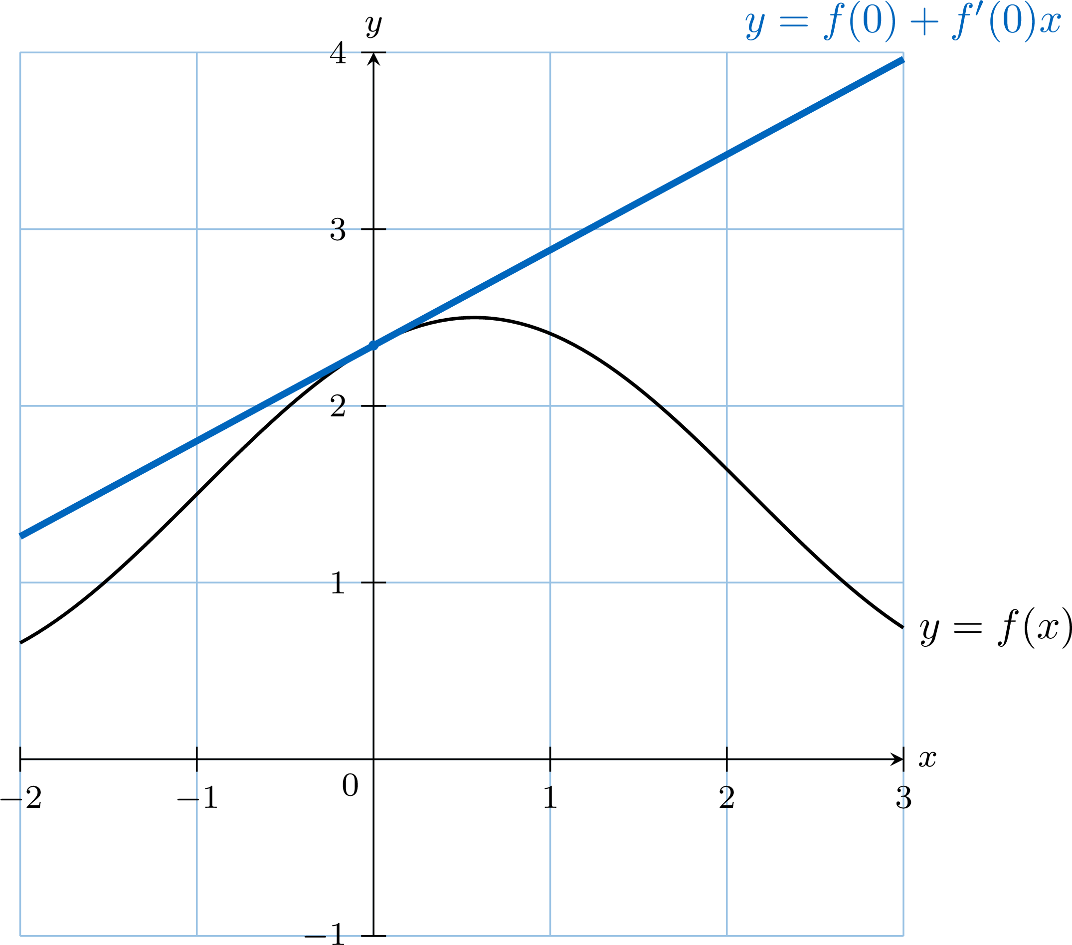
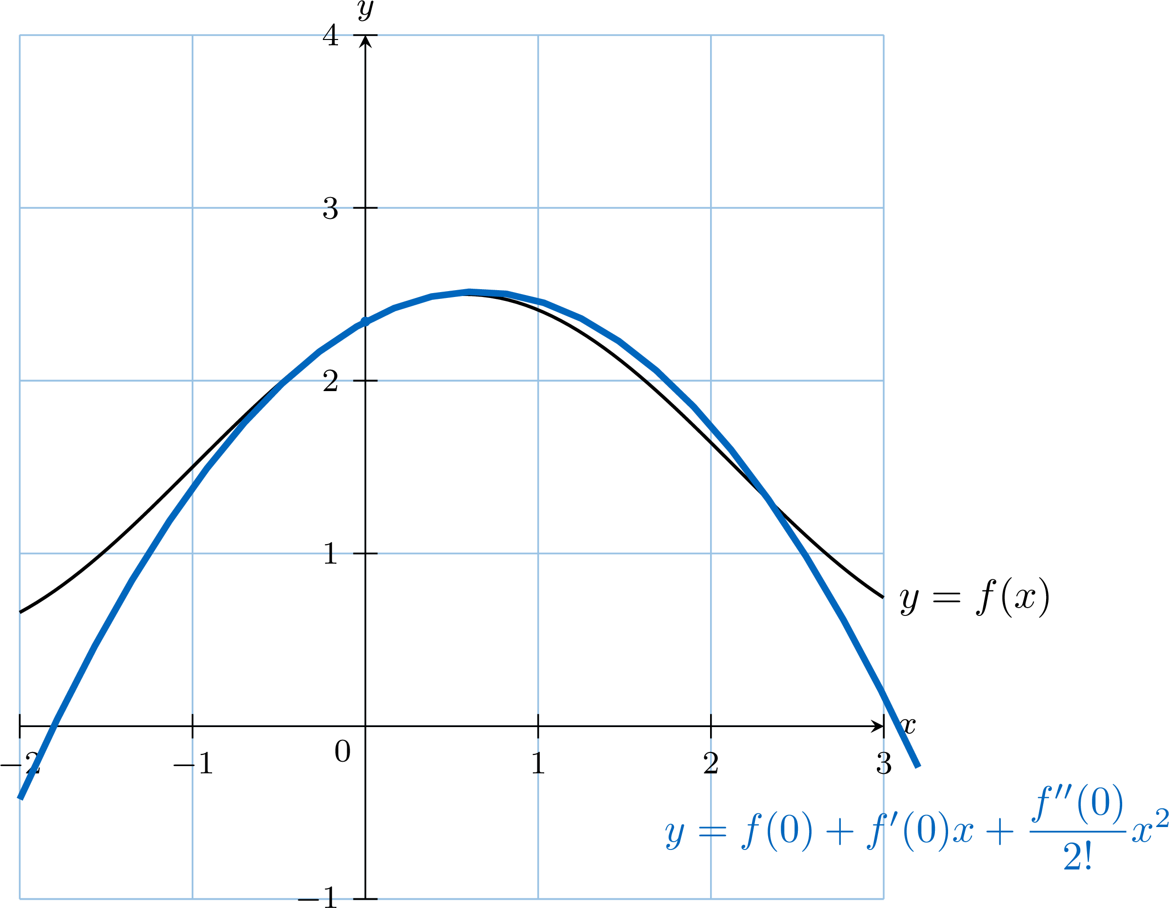
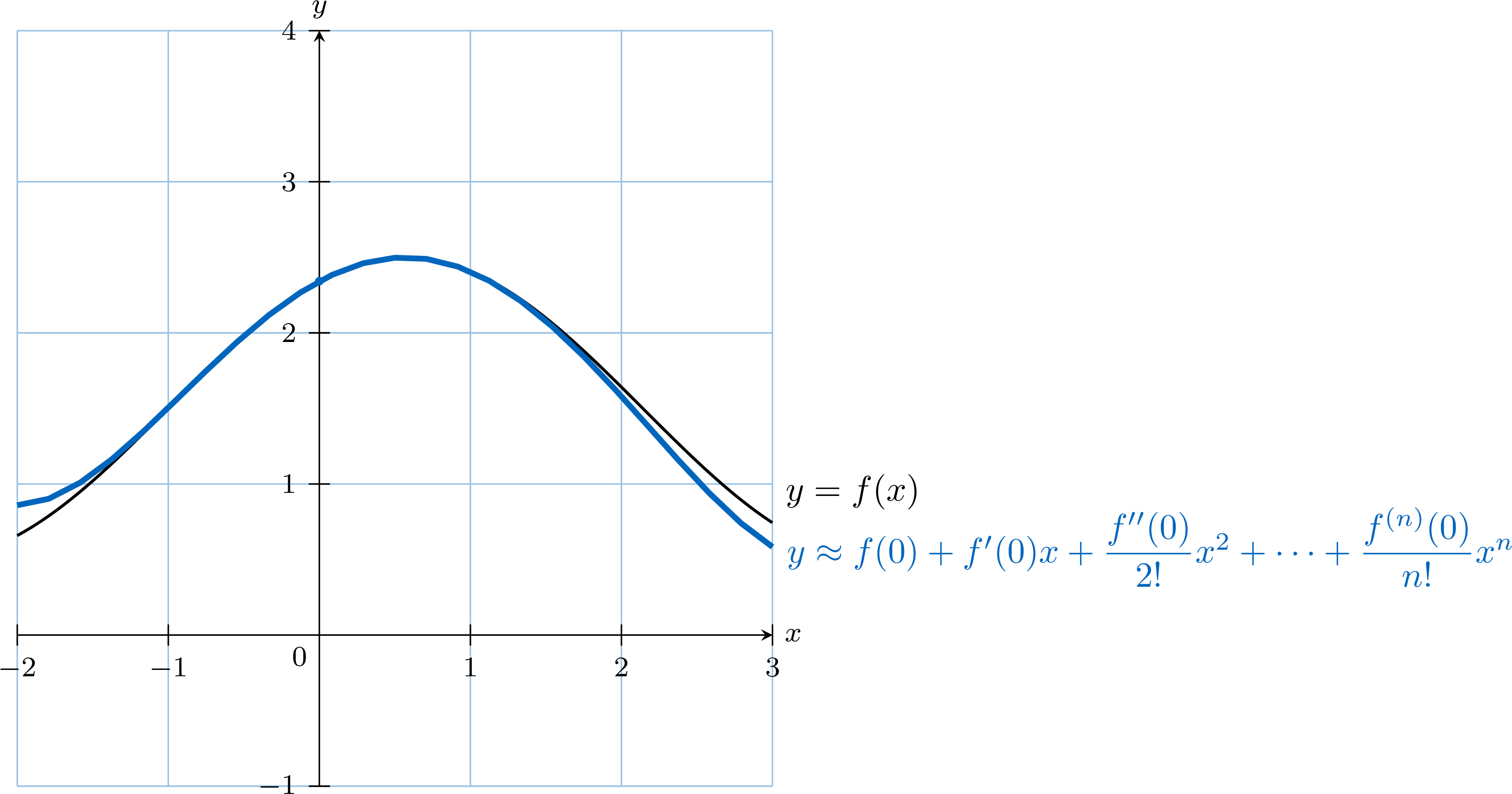
The idea of a Maclaurin series is built upon the familiar concept of linear approximation, which we can improve by adding more terms so that higher-order derivatives match at $x=0$.

Linear Approximation (Degree 1): Near $x=0$, the best linear approximation to $f(x)$ is the tangent line at that point: $$ f(x) \approx f(0) + f'(0)x. $$ This is the first Maclaurin approximation.
Quadratic Approximation (Degree 2): To get a better approximation near $x=0$, we add a quadratic term and choose its coefficient so that the second derivative of the approximation also matches that of the function at $x=0$: $$ f(x) \approx f(0) + f'(0)x + \dfrac{f''(0)}{2!}x^2. $$
Polynomial Approximation (Degree $n$): Continuing this process, a Maclaurin polynomial of degree $n$ matches the first $n$ derivatives of the function at $x=0$: $$ f(x) \approx f(0) + f'(0)x + \dfrac{f''(0)}{2!}x^2 + \dots + \dfrac{f^{(n)}(0)}{n!}x^n. $$ As $n$ increases, the polynomial “hugs’’ the function more closely near $x=0$.
The Limit: The Maclaurin Series. When we let the degree of the polynomial go to infinity and the resulting infinite series converges to $f(x)$ (for $x$ in some interval around $0$), the approximation becomes an exact equality there. This infinite series is the Maclaurin series: $$ f(x) = f(0)+f'(0)x+\dfrac{f''(0)}{2!}x^2+\dfrac{f^{(3)}(0)}{3!}x^3+\dots $$ or, in compact form, $$ f(x) = \sum_{k=0}^{\infty} \dfrac{f^{(k)}(0)}{k!}x^k. $$

Report an error

Definition — Maclaurin Series

The Maclaurin series of a function $f(x)$ that is infinitely differentiable at $x=0$ is the power series $$ \begin{aligned} f(x) &= \sum_{k=0}^{\infty} \dfrac{f^{(k)}(0)}{k!}x^k \\ &= f(0) + f'(0)x + \dfrac{f''(0)}{2!}x^2 + \dots \end{aligned} $$ Whenever this infinite series converges to $f(x)$ for $x$ in some interval around $0$, we say that $f$ is represented there by its Maclaurin series. The set of values of $x$ for which the series converges to the function value is called the interval of convergence.

Method — Finding a Maclaurin Series

To find the Maclaurin series for a function $f(x)$:

Differentiate repeatedly: Find the first few derivatives of the function: $f'(x), f''(x), f'''(x), \dots$ until a clear pattern emerges.
Evaluate at $x=0$: Calculate the value of the function and each derivative at $x=0$: $f(0), f'(0), f''(0), \dots$
Construct the series: Substitute these values into the Maclaurin series formula $$ f(x) = \sum_{k=0}^{\infty} \dfrac{f^{(k)}(0)}{k!}x^k. $$

Example

Find the Maclaurin series for the function $f(x)=e^x$.

Answer

We follow the three-step method.

Differentiate: $f(x)=e^x \implies f^{(k)}(x)=e^x$ for all $k \ge 0$.
Evaluate at $x=0$: $f^{(k)}(0) = e^0 = 1$ for all $k$.
Construct the series: $$ \begin{aligned} e^x &= \dfrac{f(0)}{0!}x^0 + \dfrac{f'(0)}{1!}x^1 + \dfrac{f''(0)}{2!}x^2 + \dots \\ &= \dfrac{1}{0!} + \dfrac{1}{1!}x + \dfrac{1}{2!}x^2 + \dfrac{1}{3!}x^3 + \dots \\ &= 1 + x + \dfrac{x^2}{2} + \dfrac{x^3}{6} + \dots \\ &= \sum_{k=0}^{\infty} \dfrac{x^k}{k!}. \end{aligned} $$

The following series are fundamental and are provided in the formula booklet.

Report an error

Proposition — Standard Maclaurin Series

$e^x$ $= \sum_{k=0}^{\infty} \dfrac{x^k}{k!} = 1 + x + \dfrac{x^2}{2!} + \dots$ for $x \in \mathbb{R}$
$\ln(1+x)$ $= \sum_{k=1}^{\infty} (-1)^{k-1}\dfrac{x^k}{k} = x - \dfrac{x^2}{2} + \dfrac{x^3}{3} - \dots$ for $-1 < x \le 1$
$\sin(x)$ $= \sum_{k=0}^{\infty} (-1)^k\dfrac{x^{2k+1}}{(2k+1)!} = x - \dfrac{x^3}{3!} + \dfrac{x^5}{5!} - \dots$ for $x \in \mathbb{R}$
$\cos(x)$ $= \sum_{k=0}^{\infty} (-1)^k\dfrac{x^{2k}}{(2k)!} = 1 - \dfrac{x^2}{2!} + \dfrac{x^4}{4!} - \dots$ for $x \in \mathbb{R}$
$\arctan(x)$ $= \sum_{k=0}^{\infty}\dfrac{ (-1)^kx^{2k+1}}{2k+1} = x - \dfrac{x^3}{3} + \dfrac{x^5}{5} - \dots$ for $|x| \le 1$
$(1+x)^p$ $= 1 + px + \dfrac{p(p-1)}{2!}x^2 + \dfrac{p(p-1)(p-2)}{3!}x^3 + \dots$ for $|x| < 1$ (for any real constant $p$)

Skills to practice

Expanding Series from Sigma Notation
Writing a Series Using Sigma Notation
Deriving Standard Series from Derivatives

II.2 Maclaurin Polynomials

Definition — Maclaurin Polynomial

A Maclaurin polynomial of degree $n$, denoted $P_n(x)$, is the finite sum of the first $n+1$ terms of the Maclaurin series, used to approximate the function near $x=0$: $$ P_n(x) = \sum_{k=0}^{n} \dfrac{f^{(k)}(0)}{k!}x^k = f(0) + f'(0)x + \dfrac{f''(0)}{2!}x^2 + \dots +\dfrac{f^{(n)}(0)}{n!}x^n. $$

Example

Find the Maclaurin polynomial of degree 4 for the function $f(x)=e^x$ and use it to approximate $e^{0.1}$.

Answer

From the previous example, the Maclaurin series for $e^x$ is $$ 1+x+\dfrac{x^2}{2!}+\dfrac{x^3}{3!}+\dfrac{x^4}{4!}+\dots $$ The Maclaurin polynomial of degree $4$ is: $$ P_4(x) = 1+x+\dfrac{x^2}{2}+\dfrac{x^3}{6}+\dfrac{x^4}{24}. $$ To approximate $e^{0.1}$, we calculate $P_4(0.1)$: $$ e^{0.1} \approx 1 + 0.1 + \dfrac{(0.1)^2}{2} + \dfrac{(0.1)^3}{6} + \dfrac{(0.1)^4}{24} \approx 1 + 0.1 + 0.005 + 0.000166\ldots + 0.000004\ldots \approx 1.10517. $$

Skills to practice

Finding and Using Maclaurin Polynomials

II.3 New Series by Substitution, Differentiation and Integration

A powerful technique is to obtain new series from ones we already know (such as the geometric series), without having to use the derivative formula from scratch every time.

Report an error

Method — Substitution

We can find the series for a composite function $f(g(x))$ by taking the series for $f(u)$ and substituting $u=g(x)$, then adjusting the interval of convergence accordingly.

Example

Starting with the geometric series $\dfrac{1}{1-u} = \sum_{k=0}^\infty u^k$ for $|u|<1$, find the Maclaurin series for $\dfrac{1}{1+x}$.

Answer

We use the geometric series formula and substitute $u = -x$. The condition $|u|<1$ becomes $|-x|<1$, which is equivalent to $|x|<1$. $$ \begin{aligned} \dfrac{1}{1-u} &= \sum_{k=0}^{\infty} u^k \\ \dfrac{1}{1-(-x)} &= \sum_{k=0}^{\infty} (-x)^k \quad(\text{letting } u=-x) \\ \dfrac{1}{1+x} &= \sum_{k=0}^{\infty} (-1)^k x^k \\ \dfrac{1}{1+x} &= 1 - x + x^2 - x^3 + \dots \quad\text{for }|x|<1. \end{aligned} $$

Method — Differentiation and Integration

We can differentiate or integrate a known Maclaurin series term-by-term within its interval of convergence to find the series for its derivative or integral.

Example

Starting with the series $\dfrac{1}{1+x} = \sum_{k=0}^\infty (-1)^k x^k$ for $|x|<1$, find the Maclaurin series for $\ln(1+x)$.

Answer

We know that $\displaystyle\int_0^u \dfrac{1}{1+x}\, \mathrm{d}x = [\ln(1+x)]_0^u = \ln(1+u)$. We integrate the series term-by-term (valid for $|u|<1$): $$ \begin{aligned} \dfrac{1}{1+x} & = 1-x+x^2-x^3+\dots \\ \int_0^u \dfrac{1}{1+x}\, \mathrm{d}x & = \int_0^u \left( 1-x+x^2-x^3+\dots\right) \, \mathrm{d}x\\ \ln(1+u) & = \int_0^u 1 \, \mathrm{d}x-\int_0^u x \, \mathrm{d}x+\int_0^u x^2 \, \mathrm{d}x-\int_0^u x^3 \, \mathrm{d}x+\dots \\ \ln(1+u) & = \left[ x\right]_0^u - \left[\dfrac{x^2}{2}\right]_0^u + \left[\dfrac{x^3}{3}\right]_0^u - \left[\dfrac{x^4}{4}\right]_0^u + \dots \\ \ln(1+u) & = u - \dfrac{u^2}{2} + \dfrac{u^3}{3} - \dfrac{u^4}{4}+\dots\\ \ln(1+x) & = x - \dfrac{x^2}{2} + \dfrac{x^3}{3} - \dfrac{x^4}{4}+\dots\quad(\text{replacing $u$ with $x$})\\ \ln(1+x) & = \sum_{k=1}^\infty (-1)^{k-1}\dfrac{x^k}{k},\quad |x|<1. \end{aligned} $$

Example

Starting with the geometric series $\dfrac{1}{1-x} = \sum_{k=0}^\infty x^k$ for $|x|<1$, find the Maclaurin series for $\dfrac{1}{(1-x)^2}$.

Answer

We know that $\dfrac{d}{\mathrm{d}x}\left(\dfrac{1}{1-x}\right) = \dfrac{1}{(1-x)^2}$. We differentiate the series term-by-term (valid for $|x|<1$): $$ \begin{aligned} \dfrac{1}{1-x} & = 1+x+x^2+x^3+x^4+\dots \\ \dfrac{d}{\mathrm{d}x}\left(\dfrac{1}{1-x}\right) & = \dfrac{d}{\mathrm{d}x}\left( 1+x+x^2+x^3+x^4+\dots\right) \\ \dfrac{1}{(1-x)^2} & = \dfrac{d}{\mathrm{d}x}\left( 1\right)+\dfrac{d}{\mathrm{d}x}\left(x\right)+\dfrac{d}{\mathrm{d}x}\left(x^2\right)+\dfrac{d}{\mathrm{d}x}\left(x^3\right)+\dfrac{d}{\mathrm{d}x}\left(x^4\right)+\dots \\ \dfrac{1}{(1-x)^2} & = 0 + 1 + 2x + 3x^2 + 4x^3 + \dots \\ \dfrac{1}{(1-x)^2} & = \sum_{k=0}^\infty (k+1)x^k,\quad |x|<1. \end{aligned} $$

Skills to practice

Finding New Series by Substitution
Finding Series with the Binomial Series
Differentiating and Integrating Maclaurin Polynomials
Finding New Series by Differentiation or Integration

II.4 Sums, Multiples and Products of Series

Maclaurin series behave like polynomials: they can be added, subtracted, and multiplied by constants term-by-term. The resulting series will converge on the intersection of the intervals of convergence of the individual series.

Report an error

Proposition — Linearity Property

If the Maclaurin series for $f(x)$ and $g(x)$ are known, and $c$ is a constant, then:

Sum/Difference: The series for $f(x) \pm g(x)$ is the term-by-term sum/difference of their respective series.
Scalar Multiple: The series for $c \cdot f(x)$ is the series for $f(x)$ with each term multiplied by $c$.

Example

Find the Maclaurin series for $f(x) = \cosh(x)$ up to the term in $x^4$, using the series for $e^x$ and $e^{-x}$. (Recall that $\cosh(x) = \dfrac{e^x + e^{-x}}{2}$.)

Answer

First, we write out the series for $e^x$ and find the series for $e^{-x}$ by substitution: $$ e^x = 1 + x + \dfrac{x^2}{2!} + \dfrac{x^3}{3!} + \dfrac{x^4}{4!} + \dots $$ $$ e^{-x} = 1 - x + \dfrac{x^2}{2!} - \dfrac{x^3}{3!} + \dfrac{x^4}{4!} - \dots $$ Now, we add the two series together. Notice that the odd-powered terms cancel out: $$ \begin{aligned} e^x + e^{-x} &= (1+1) + (x-x) + \left(\dfrac{x^2}{2!}+\dfrac{x^2}{2!}\right) + \left(\dfrac{x^3}{3!}-\dfrac{x^3}{3!}\right) + \left(\dfrac{x^4}{4!}+\dfrac{x^4}{4!}\right) + \dots \\ &= 2 + 2\dfrac{x^2}{2!} + 2\dfrac{x^4}{4!} + \dots \end{aligned} $$ Finally, we multiply the entire series by the scalar $\dfrac{1}{2}$: $$ \cosh(x) = \dfrac{e^x + e^{-x}}{2} = \dfrac{1}{2}\left(2 + 2\dfrac{x^2}{2!} + 2\dfrac{x^4}{4!} + \dots\right) = 1 + \dfrac{x^2}{2!} + \dfrac{x^4}{4!} + \dots $$ So, up to the term in $x^4$, $$ \cosh(x) \approx 1 + \dfrac{x^2}{2} + \dfrac{x^4}{24}. $$

Maclaurin series are multiplied like polynomials: each term of one series by each term of the other. Since only the first terms are wanted, the products whose power of $x$ exceeds the last power asked for are simply not written: each coefficient of the product needs only a few terms of each factor.

Report an error

Method — Multiplying Two Maclaurin Series

To find the Maclaurin series of $f(x)g(x)$ up to the term in $x^m$:

Write each series up to $x^m$: $f(x) = a_0 + a_1x + a_2x^2 + \dotsb$ and $g(x) = b_0 + b_1x + b_2x^2 + \dotsb$
Collect the coefficient of each power $x^k$, $k \leq m$, from the products of a term of $f$ and a term of $g$ whose powers add up to $k$: $$f(x)g(x) = a_0b_0 + (a_0b_1 + a_1b_0)x + (a_0b_2 + a_1b_1 + a_2b_0)x^2 + \dotsb$$
State the interval of validity: the product series is valid inside the interval where both series are valid (an end point of that interval needs a separate check).

A quotient $\dfrac{f(x)}{1 + u(x)}$, where $f$ and $u$ have Maclaurin series and $u(0) = 0$, is the product of $f(x)$ and $\big(1 + u(x)\big)^{-1}$, whose series comes from the binomial theorem; the series found is valid for $x$ close enough to $0$ (its exact interval of validity is not studied here).

Example

Find the Maclaurin series of $e^x\sin x$ up to the term in $x^5$.

Answer

The standard series, valid for every real $x$, are $$e^x = 1 + x + \frac{x^2}{2} + \frac{x^3}{6} + \frac{x^4}{24} + \dotsb \quad\text{and}\quad \sin x = x - \frac{x^3}{6} + \frac{x^5}{120} - \dotsb$$ Every term of $\sin x$ contains $x$, so the powers up to $x^5$ need $e^x$ up to $x^4$. Coefficient by coefficient: $$\begin{aligned}[t] x &: \ 1 \times 1 = 1 &&\text{($1 \cdot x$)}\\ x^2 &: \ 1 \times 1 = 1 &&\text{($x \cdot x$)}\\ x^3 &: \ 1 \times \left(-\frac{1}{6}\right) + \frac{1}{2} \times 1 = \frac{1}{3} &&\text{($1 \cdot x^3$, $x^2 \cdot x$)}\\ x^4 &: \ 1 \times \left(-\frac{1}{6}\right) + \frac{1}{6} \times 1 = 0 &&\text{($x \cdot x^3$, $x^3 \cdot x$)}\\ x^5 &: \ \frac{1}{120} + \frac{1}{2} \times \left(-\frac{1}{6}\right) + \frac{1}{24} \times 1 = -\frac{1}{30} &&\text{($1 \cdot x^5$, $x^2 \cdot x^3$, $x^4 \cdot x$)} \end{aligned}$$ (in brackets, the powers of $e^x$ and of $\sin x$ that are multiplied). Hence, for every real $x$, $$e^x\sin x = x + x^2 + \frac{x^3}{3} - \frac{x^5}{30} + \dotsb$$

Example

Find the Maclaurin series of $\dfrac{e^x}{1 - x}$ up to the term in $x^3$, and state where it is valid.

Answer

Write the quotient as a product: $\dfrac{e^x}{1 - x} = e^x \times (1 - x)^{-1}$, with the geometric series $(1 - x)^{-1} = 1 + x + x^2 + x^3 + \dotsb$ for $|x| < 1$. Then $$\begin{aligned}[t] \frac{e^x}{1 - x} &= \left(1 + x + \frac{x^2}{2} + \frac{x^3}{6} + \dotsb\right)\left(1 + x + x^2 + x^3 + \dotsb\right)\\ &= 1 + (1 + 1)x + \left(1 + 1 + \frac{1}{2}\right)x^2 + \left(1 + 1 + \frac{1}{2} + \frac{1}{6}\right)x^3 + \dotsb &&\text{(collect each power)}\\ &= 1 + 2x + \frac{5}{2}x^2 + \frac{8}{3}x^3 + \dotsb \end{aligned}$$ The series of $e^x$ is valid for every real $x$ and the geometric series for $|x| < 1$: the product is valid for $-1 < x < 1$. Each coefficient is the sum $1 + 1 + \dfrac{1}{2!} + \dotsb + \dfrac{1}{k!}$ of the first coefficients of $e^x$.

Skills to practice

Multiplying Maclaurin Series
Combining Series

II.5 Limits Using Maclaurin Series

Method — Evaluating a Limit with Maclaurin Series

To find the limit as $x \to 0$ of a quotient $\dfrac{f(x)}{g(x)}$ of the indeterminate form $\dfrac{0}{0}$ (L'Hôpital's rule is the other route):

Replace each function by its Maclaurin series, with enough terms to reach the first non-zero term of the numerator and of the denominator.
Simplify the expression: for $x \neq 0$, factor the lowest power of $x$ out of the numerator and the denominator, and cancel it.
Let $x \to 0$: every remaining term that contains a positive power of $x$ tends to $0$, and the limit is read on the constant terms. If a negative power of $x$ remains (the lowest power of the denominator is higher than the lowest power of the numerator), the quotient has no finite limit.

The expression is transformed first; the arrow comes last, on the simplified form.

Example

Find $\displaystyle\lim_{x \to 0} \frac{1 - \cos x}{x^2}$.

Answer

With $\cos x = 1 - \dfrac{x^2}{2} + \dfrac{x^4}{24} - \dotsb$, for $x \neq 0$: $$\begin{aligned}[t] \frac{1 - \cos x}{x^2} &= \frac{\dfrac{x^2}{2} - \dfrac{x^4}{24} + \dotsb}{x^2} &&\text{(series of $\cos x$)}\\ &= \frac{1}{2} - \frac{x^2}{24} + \dotsb &&\text{(divide by $x^2$)}\\ &\xrightarrow[x \to 0]{} \frac{1}{2}. \end{aligned}$$ Hence $\displaystyle\lim_{x \to 0} \frac{1 - \cos x}{x^2} = \frac{1}{2}$.

Example

Find $\displaystyle\lim_{x \to 0} \frac{x - \sin x}{x^3}$, first with Maclaurin series, then with L'Hôpital's rule.

Answer

With series. With $\sin x = x - \dfrac{x^3}{6} + \dfrac{x^5}{120} - \dotsb$, for $x \neq 0$: $$\begin{aligned}[t] \frac{x - \sin x}{x^3} &= \frac{\dfrac{x^3}{6} - \dfrac{x^5}{120} + \dotsb}{x^3} &&\text{(series of $\sin x$)}\\ &= \frac{1}{6} - \frac{x^2}{120} + \dotsb\\ &\xrightarrow[x \to 0]{} \frac{1}{6}. \end{aligned}$$ With L'Hôpital's rule. The quotients $\dfrac{x - \sin x}{x^3}$, $\dfrac{1 - \cos x}{3x^2}$ and $\dfrac{\sin x}{6x}$ are all of the form $\dfrac{0}{0}$ at $0$, so the rule is applied three times, until $\dfrac{\cos x}{6} \xrightarrow[x \to 0]{} \dfrac{1}{6}$. The series reach the same value $\dfrac{1}{6}$ in one step: its $\dfrac{1}{6}$ is the coefficient of $x^3$ in the series of $\sin x$, up to the sign.

Skills to practice

Evaluating Limits with Series
Justifying Limits with Series

III Going further

Skills to practice

Writing Mathematics
Solving Problems
Quiz