International Baccalaureate · DP 2: Analysis and Approaches HL
Limits and Continuity
I
Limits of Functions
I.1
The Limit of a Function
The ancient Greek philosopher Zeno of Elea famously argued that motion was impossible. In his paradox of Achilles and the Tortoise, the swift hero Achilles can never overtake a slow tortoise given a head start, because by the time Achilles reaches the tortoise's starting point, the tortoise has already moved a little further ahead. When Achilles covers that new distance, the tortoise has moved ahead again. This process repeats endlessly, suggesting Achilles can never close the gap.
This paradox highlights a profound mathematical problem: how do we handle the infinitely small and the concept of "approaching" a value? It took mathematicians like Augustin-Louis Cauchy and Karl Weierstrass over two millennia to formalize the answer with the concept of the limit. A limit describes the value a function "approaches" as its input gets closer and closer to a certain point. It is a foundational concept in calculus, because it underlies the definitions of both derivatives and integrals.
This paradox highlights a profound mathematical problem: how do we handle the infinitely small and the concept of "approaching" a value? It took mathematicians like Augustin-Louis Cauchy and Karl Weierstrass over two millennia to formalize the answer with the concept of the limit. A limit describes the value a function "approaches" as its input gets closer and closer to a certain point. It is a foundational concept in calculus, because it underlies the definitions of both derivatives and integrals.
Definition — Limit
A function \(f\) has the limit \(L\) as \(x\) approaches \(a\) if the values of \(f(x)\) become arbitrarily close to the single real number \(L\) whenever \(x\) is sufficiently close to \(a\), with \(x \neq a\), from both sides. We write this as:$$ \textcolor{colordef}{\lim_{x \to a} f(x) = L}\quad\text{or}\quad\textcolor{colordef}{f(x) \xrightarrow[x \to a]{} L}\quad\text{or}\quad\textcolor{colordef}{\text{as } x \to a,\ f(x)\to L}$$
The crucial idea of a limit is that it describes the behaviour of a function near a point, not at the point itself. The value of \(f(a)\), or whether it even exists, is irrelevant to the value of the limit.
Consider the function \(f(x) = \dfrac{x^2-1}{x-1}\). At \(x=1\), the function is undefined. However, for any \(x \neq 1\), we can simplify:$$ f(x) = \dfrac{(x-1)(x+1)}{x-1} = x+1. $$ The graph of \(f(x)\) is the line \(y=x+1\) with a "hole" at \(x=1\). As \(x\) gets very close to 1 from either side, the value of \(f(x)\) gets very close to 2. Therefore, \(\displaystyle\lim_{x \to 1} f(x) = 2\), even though \(f(1)\) is not defined. 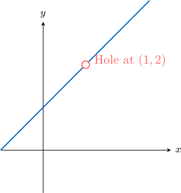
Consider the function \(f(x) = \dfrac{x^2-1}{x-1}\). At \(x=1\), the function is undefined. However, for any \(x \neq 1\), we can simplify:$$ f(x) = \dfrac{(x-1)(x+1)}{x-1} = x+1. $$ The graph of \(f(x)\) is the line \(y=x+1\) with a "hole" at \(x=1\). As \(x\) gets very close to 1 from either side, the value of \(f(x)\) gets very close to 2. Therefore, \(\displaystyle\lim_{x \to 1} f(x) = 2\), even though \(f(1)\) is not defined.
Example
- Complete, with a calculator, a table of values of \(f(x) = \dfrac{e^x - 1}{x}\) for \(x = \pm 0.1\), \(\pm 0.01\), \(\pm 0.001\), and estimate \(\displaystyle\lim_{x \to 0} f(x)\).
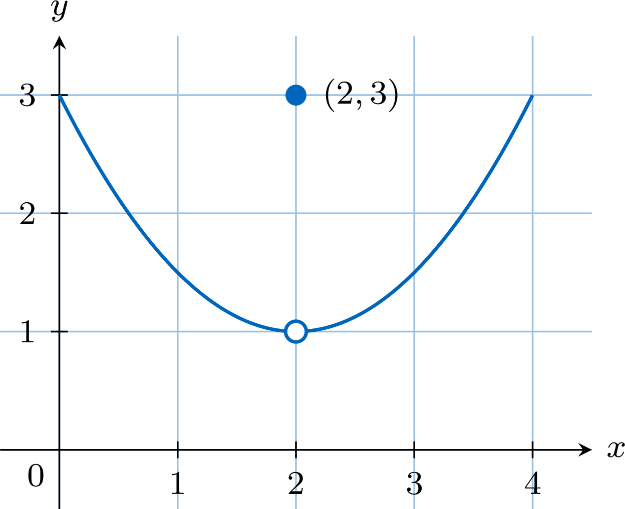
- The curve of a function \(g\) defined on \([0, 4]\) is drawn below. Estimate \(\displaystyle\lim_{x \to 2} g(x)\), and compare it with \(g(2)\).
- \(f(0)\) is not defined (numerator and denominator are both \(0\) at \(x = 0\)), so the table approaches \(0\) from both sides (values to \(5\) decimal places):
\(x\) \(-0.1\) \(-0.01\) \(-0.001\) \(0.001\) \(0.01\) \(0.1\) \(f(x)\) \(0.95163\) \(0.99502\) \(0.99950\) \(1.00050\) \(1.00502\) \(1.05171\) - As \(x\) gets closer to \(2\), from either side, the points of the curve get closer to the hole at \((2, 1)\): \(\displaystyle\lim_{x \to 2} g(x) = 1\). The isolated point shows that \(g(2) = 3\). The limit describes the values of \(g\) near \(2\), not at \(2\): here \(\displaystyle\lim_{x \to 2} g(x) \neq g(2)\).
Skills to practice
- Estimating Limits from Tables and Graphs
I.2
One-Sided Limits and Vertical Asymptotes
Definition — One-Sided Limits
- The right-hand limit, \(\displaystyle\lim_{x \to a^+} f(x)\), is the value that \(f(x)\) approaches as \(x\) approaches \(a\) from values greater than \(a\).
- The left-hand limit, \(\displaystyle\lim_{x \to a^-} f(x)\), is the value that \(f(x)\) approaches as \(x\) approaches \(a\) from values less than \(a\).
Proposition — Existence of a Limit
When \(f\) is defined on both sides of \(a\), the two-sided limit \(\displaystyle\lim_{x \to a} f(x)\) exists if and only if the left-hand and right-hand limits both exist and are equal:$$ \displaystyle\lim_{x \to a} f(x) = L \iff \displaystyle\lim_{x \to a^-} f(x) = L \text{ and } \displaystyle\lim_{x \to a^+} f(x) = L $$ Example
Consider the piecewise function \(f(x) = \begin{cases} x, & x < 1 \\ x^2, & x \ge 1 \end{cases}\). Does \(\lim_{x \to 1} f(x)\) exist?
To determine if the limit exists, we must find the left-hand and right-hand limits and check if they are equal. 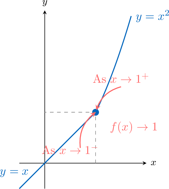
- Left-hand limit: As \(x \to 1^-\), we use the rule for \(x<1\).$$ \lim_{x \to 1^-} f(x) = \lim_{x \to 1^-} (x) = 1 $$
- Right-hand limit: As \(x \to 1^+\), we use the rule for \(x \ge 1\).$$ \lim_{x \to 1^+} f(x) = \lim_{x \to 1^+} (x^2) = 1^2 = 1 $$
Example
Consider the piecewise function \(f(x) = \begin{cases} x+1, & x < 1 \\ x^2, & x \ge 1 \end{cases}\). Does \(\lim_{x \to 1} f(x)\) exist?
To determine if the limit exists, we must find the left-hand and right-hand limits and check if they are equal. 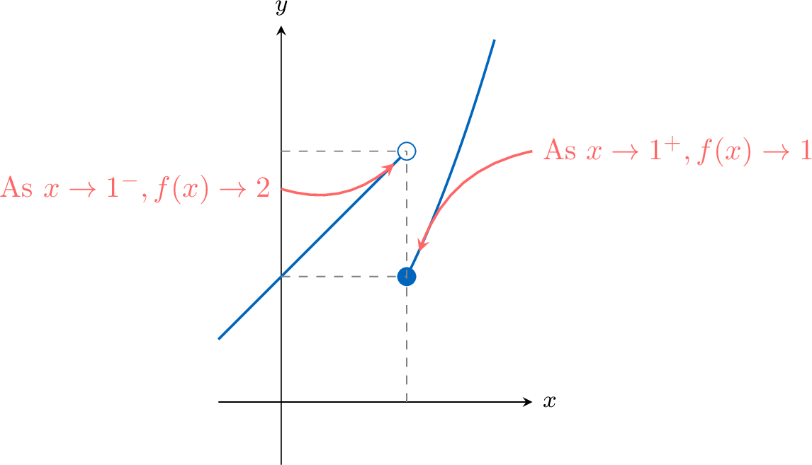
- Left-hand limit: As \(x \to 1^-\), we use the rule for \(x<1\).$$ \lim_{x \to 1^-} f(x) = \lim_{x \to 1^-} (x+1) = 1+1 = 2 $$
- Right-hand limit: As \(x \to 1^+\), we use the rule for \(x \ge 1\).$$ \lim_{x \to 1^+} f(x) = \lim_{x \to 1^+} (x^2) = 1^2 = 1 $$
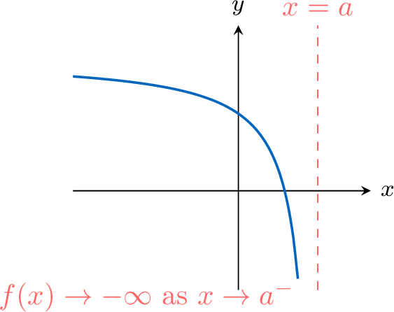
A function may also have an infinite limit at a point: its values grow without bound, approaching \(+\infty\) or \(-\infty\), as \(x\) approaches \(a\). While these limits do not technically exist as finite numbers, we use limit notation as a precise way to describe this "unbounded behaviour," which corresponds to a vertical asymptote on a graph.
Definition — Infinite Limit
The notation \(\displaystyle\lim_{x \to a} f(x) = +\infty\) means that the values of \(f(x)\) can be made arbitrarily large and positive by taking \(x\) sufficiently close to \(a\), with \(x \neq a\) (from both sides).Similarly for \(\displaystyle\lim_{x \to a} f(x) = -\infty\).
In this situation we say that the limit diverges to \(+\infty\) or \(-\infty\); it is not a finite real number.
Definition — Vertical Asymptote
The line \(x=a\) is a vertical asymptote of the graph of the function \(f(x)\) if the function approaches \(+\infty\) or \(-\infty\) as \(x\) approaches \(a\) from the left or the right. 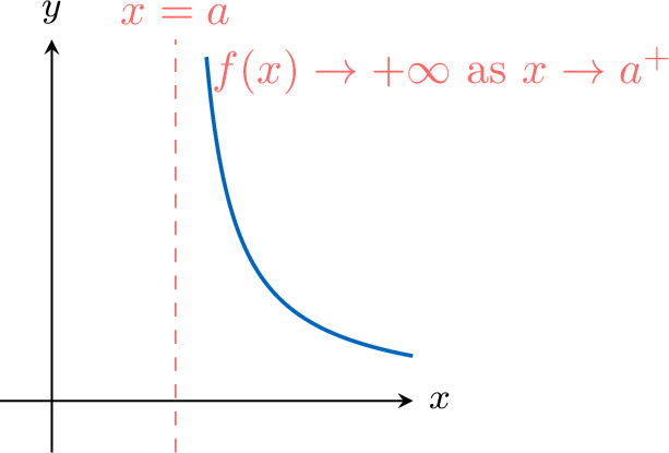
Example
Investigate \(\displaystyle\lim_{x \to 0} \dfrac{1}{x^2}\).
The expression \(\dfrac{1}{x^2}\) is not defined at \(x=0\); this alone decides nothing (compare \(\dfrac{x^2-1}{x-1}\) at \(1\)), so we check the one-sided limits: 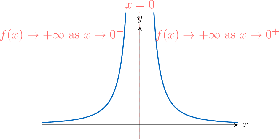
- As \(x \to 0^+\), \(x^2\) is a small positive number, so \(\dfrac{1}{x^2} \to +\infty\).
- As \(x \to 0^-\), \(x^2\) is also a small positive number, so \(\dfrac{1}{x^2} \to +\infty\).
The Notation \(0^+\) and \(0^-\)
When a denominator tends to \(0\), knowing this alone is not enough to conclude: the limit of \(\dfrac{1}{x}\) at \(0\) is \(+\infty\) on the right and \(-\infty\) on the left. When the numerator has a non-zero limit, the sign of the denominator near the point decides. We write $$g(x) \to \mathbf{0^+} \qquad \text{(resp. } g(x) \to \mathbf{0^-}\text{)}$$ when \(g(x)\) tends to \(0\) while staying strictly positive (resp. strictly negative) near the point considered. Then, if \(f(x) \to L\) with \(L > 0\): \(\dfrac{f(x)}{g(x)} \to +\infty\) if \(g(x) \to 0^+\) and \(\dfrac{f(x)}{g(x)} \to -\infty\) if \(g(x) \to 0^-\) (and the opposite signs for \(L < 0\)). This is the meaning of the sign rule in the property « Operations on Limits ». When the denominator changes sign at the point, the limits on the left and on the right are studied separately, provided its sign is constant on each side.
Skills to practice
- Determining One-Sided Limits
I.3
Limits at Infinity and Horizontal Asymptotes
Limits at infinity describe the behaviour at infinity of a function. When \(\displaystyle\lim_{x \to +\infty} f(x) = L\) (or \(\displaystyle\lim_{x \to -\infty} f(x) = L\)), the line \(y=L\) is a horizontal asymptote of the graph.
Definition — Limit at Infinity
A function \(f\) has the limit \(L\) as \(x\) approaches \(+\infty\) when the values of \(f(x)\) become arbitrarily close to the single real number \(L\) for all sufficiently large \(x\). We write:$$ \textcolor{colordef}{\lim_{x \to +\infty} f(x) = L}\quad\text{or}\quad\textcolor{colordef}{f(x) \xrightarrow[x \to +\infty]{} L}. $$ 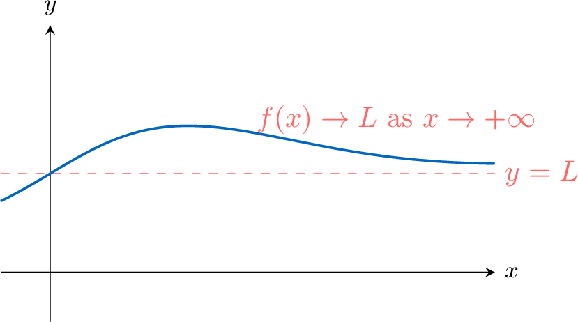
Definition — Horizontal Asymptote
The line \(y=L\) is a horizontal asymptote of the graph of the function \(f(x)\) if either of the following limit conditions is met:$$ \lim_{x \to +\infty} f(x) = L \quad \text{or} \quad \lim_{x \to -\infty} f(x) = L $$ Example
The curve \(\mathcal{C}\) below is the curve of a function \(f\) defined on \(]-\infty\,;\,0[ \cup ]0\,;\,+\infty[\). Read the limits of \(f\) at \(+\infty\) and at \(-\infty\), and give the horizontal asymptote of \(\mathcal{C}\). 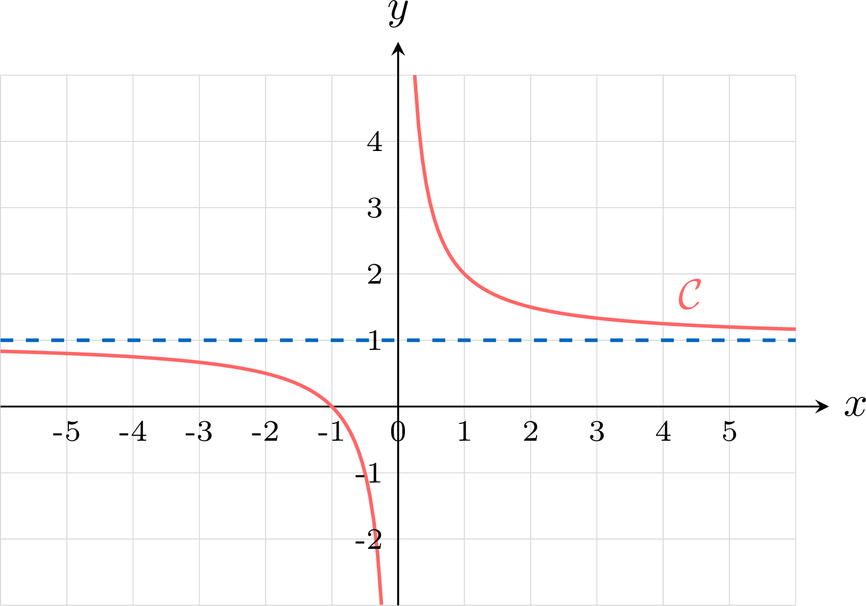
As \(x\) takes larger and larger values, the points of \(\mathcal{C}\) get closer and closer to the dashed line \(y = 1\), from above: the values \(f(x)\) become arbitrarily close to \(1\) as soon as \(x\) is large enough. So \(\displaystyle \lim_{x \to +\infty} f(x) = 1\). In the same way, as \(x\) takes smaller and smaller values, the points of \(\mathcal{C}\) get closer and closer to the same line, from below: \(\displaystyle \lim_{x \to -\infty} f(x) = 1\). The line \(y = 1\) is a horizontal asymptote of \(\mathcal{C}\) at \(+\infty\) and at \(-\infty\).
Definition — Infinite Limit at Infinity
Let \(f\) be a function defined on an interval \([a\,;\,+\infty[\). The function \(f\) has the limit \(+\infty\) as \(x\) approaches \(+\infty\) when every interval \(]A\,;\,+\infty[\) (where \(A\) is a real number) contains all the values \(f(x)\) for \(x\) large enough, that is for all the \(x\) greater than some real number \(x_A\). In other words, \(f(x)\) can be made as large as we want by taking \(x\) large enough. We write: $$\lim_{x \to +\infty} f(x) = +\infty.$$ 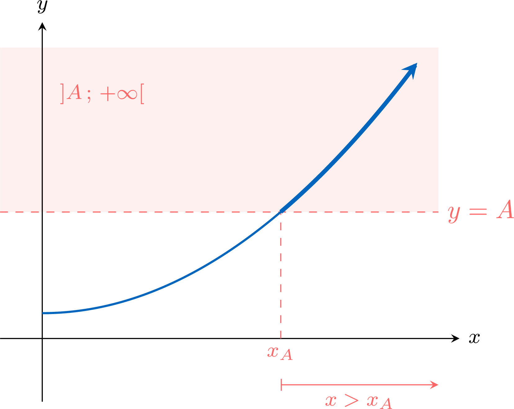
Skills to practice
- Estimating Limits at Infinity
- Investigating Infinite Limits Numerically
I.4
Calculating Limits
Proposition — Reference Limits
The following limits for standard functions are used as building blocks for more complex calculations: | Function | \(\mathbf{x \to -\infty}\) | \(\mathbf{x \to +\infty}\) | \(\mathbf{x \to 0^-}\) | \(\mathbf{x \to 0^+}\) |
| \(1/x\) | \(0\) | \(0\) | \(-\infty\) | \(+\infty\) |
| \(x^n\) (\(n \in \mathbb{N}^*\)) | \(+\infty\) (even) / \(-\infty\) (odd) | \(+\infty\) | 0 | 0 |
| \(e^x\) | \(0\) | \(+\infty\) | 1 | 1 |
| \(\sqrt{x}\) | Undefined | \(+\infty\) | Undefined | \(0\) |
| \(1/\sqrt{x}\) | Undefined | \(0\) | Undefined | \(+\infty\) |
While tables of values and graphs are useful for understanding the concept of a limit, they are not efficient for evaluation. Fortunately, limits follow a set of predictable algebraic rules, known as the operations on limits, which allow us to calculate them directly.
Proposition — Operations on Limits
Let \(L\) and \(L'\) be real numbers. The following tables summarize the rules for limits of sums, products, and quotients involving infinity. - Sum and Product:
\(\lim f(x)\) \(\lim g(x)\) \(\lim (f(x)+g(x))\) \(\lim (f(x) \times g(x))\) \(L\) \(L'\) \(L+L'\) \(L \times L'\) \(L\neq 0\) \(\pm \infty\) \(\pm \infty\) \(\pm \infty\) (sign rule) \(\pm \infty\) \(\pm \infty\) \(\pm \infty\) (if same sign) \(\pm \infty\) (sign rule) \(0\) \(\pm \infty\) \(\pm \infty\) Indeterminate Form \(+\infty\) \(-\infty\) Indeterminate Form \(-\infty\) - Quotient:
\(\lim f(x)\) \(\lim g(x)\) \(\lim \dfrac{f(x)}{g(x)}\) \(L\) \(L' \neq 0\) \(\dfrac{L}{L'}\) \(L\) \(\pm \infty\) \(0\) \(L \neq 0\) \(0^+\) or \(0^-\) (denominator of constant sign) \(\pm \infty\) (sign rule) \(\pm \infty\) \(L' \neq 0\) \(\pm \infty\) (sign rule) \(0\) \(0\) Indeterminate Form \(\pm \infty\) \(\pm \infty\) Indeterminate Form
Limit at a Point Where the Function Is Defined
For the usual functions listed in the Method “Evaluating Limits” (polynomial and rational functions, square root, exponential, and the functions built from them by the operations), the limit at a point \(a\) of the domain is the value \(f(a)\). This property is admitted here: it expresses that these functions are continuous, a notion studied with continuity.
For such functions, the only real numbers that need a separate study are those where the function is not defined (a zero of a denominator, for instance). At a boundary point of the domain, such as \(0\) for the square root function, the limit is studied from inside the domain only.
For such functions, the only real numbers that need a separate study are those where the function is not defined (a zero of a denominator, for instance). At a boundary point of the domain, such as \(0\) for the square root function, the limit is studied from inside the domain only.
Method — Evaluating Limits
- Direct Substitution (when \(a\) is a real number): When \(a\) is a real number, start by substituting \(x=a\) into \(f(x)\) (at \(\pm\infty\), use the operations on limits and the dominant terms instead).
- If the expression is defined at \(x=a\) (no division by \(0\), no square root of a negative number, etc.) and the function is continuous at \(a\) (as is the case for polynomials, rational functions where the denominator is nonzero, \(e^x\), etc.), then: $$ \lim_{x\to a} f(x)=f(a). $$
- If the expression is not defined, or if the function may have a discontinuity, direct substitution is not sufficient: we must transform the expression or study one-sided limits.
- Algebraic Manipulation: If substitution leads to an indeterminate form such as \(\dfrac{0}{0}\), simplify the expression by:
- factoring and cancelling common factors (when allowed);
- using a conjugate (for expressions with roots);
- rewriting the expression (common denominator, factoring out dominant terms, etc.).
Example
Evaluate the following limits: - \(\displaystyle\lim_{x \to 2} \frac{x^2-5x+6}{x-2}\);
- \(\displaystyle\lim_{x \to +\infty} \frac{2x^2+5x}{3x^2-1}\);
- \(\displaystyle\lim_{x \to 0} \frac{\sqrt{x+4}-2}{x}\).
Each limit is an indeterminate form: we first transform the expression (the limit may not exist yet!), and only pass to the limit once the indeterminacy is gone.
- Factor and cancel (form \(\frac{0}{0}\)): for \(x \neq 2\), $$\frac{x^2-5x+6}{x-2} = \frac{(x-2)(x-3)}{x-2} = x-3 \xrightarrow[x \to 2]{} -1.$$
- Dominant terms (form \(\frac{\infty}{\infty}\)): factoring out the dominant term \(x^2\) on top and bottom, then cancelling, for \(x \neq 0\), $$\frac{2x^2+5x}{3x^2-1} = \frac{x^2\left(2+\frac{5}{x}\right)}{x^2\left(3-\frac{1}{x^2}\right)} = \frac{\cancel{x^2}\left(2+\frac{5}{x}\right)}{\cancel{x^2}\left(3-\frac{1}{x^2}\right)} \xrightarrow[x \to +\infty]{} \frac{2+0}{3-0} = \frac{2}{3}.$$
- Conjugate (form \(\frac{0}{0}\)): multiplying by \(\frac{\sqrt{x+4}+2}{\sqrt{x+4}+2}\), for \(x \neq 0\), $$\frac{\sqrt{x+4}-2}{x} = \frac{(x+4)-4}{x\left(\sqrt{x+4}+2\right)} = \frac{1}{\sqrt{x+4}+2} \xrightarrow[x \to 0]{} \frac{1}{2+2} = \frac{1}{4}.$$
Caution: Direct substitution is reliable for continuous functions. However, if a function has a discontinuity (a “jump”), a hole, or different formulas on either side of a point (such as a function defined piecewise, for instance \(f(x) = x + 1\) for \(x < 1\) and \(f(x) = x^2\) for \(x \geq 1\)), substitution can be misleading. In that case, study one-sided limits or transform the expression first.
Method — Determining the Asymptotes of a Curve
Let \(f\) be a function built from the usual functions and \(\mathcal{C}\) its curve. - Horizontal asymptote. Determine the limit of \(f\) at \(+\infty\) and at \(-\infty\), when the domain extends there. If \(f(x) \xrightarrow[x \to +\infty]{} \ell\) (a real number), the line \(y = \ell\) is a horizontal asymptote of \(\mathcal{C}\) at \(+\infty\); likewise at \(-\infty\).
- Vertical asymptote. Determine the limit of \(f\) at each real number \(a\) where \(f\) is not defined but which can be approached from inside the domain (a zero of a denominator, for instance), on the left and on the right when both sides belong to the domain. If one of these limits is \(+\infty\) or \(-\infty\), the line \(x = a\) is a vertical asymptote of \(\mathcal{C}\).
- Position of the curve. Study the sign of \(f(x) - \ell\) to know whether \(\mathcal{C}\) lies above or below its horizontal asymptote.
Example
Let \(f(x) = \dfrac{3x + 2}{x - 1}\) for every real number \(x \neq 1\), and let \(\mathcal{C}\) be its curve. Determine the asymptotes of \(\mathcal{C}\), then the position of \(\mathcal{C}\) with respect to its horizontal asymptote. - At \(+\infty\) and \(-\infty\). Numerator and denominator both tend to \(+\infty\) at \(+\infty\) (resp. to \(-\infty\) at \(-\infty\)): indeterminate form. For \(x \neq 0\), factor the dominant term \(x\): $$\begin{aligned} f(x) &= \frac{3x + 2}{x - 1} \\ &= \frac{x\left(3 + \frac{2}{x}\right)}{x\left(1 - \frac{1}{x}\right)} && \text{(factor } x\text{)} \\ &= \frac{\cancel{x}\left(3 + \frac{2}{x}\right)}{\cancel{x}\left(1 - \frac{1}{x}\right)} && \text{(simplify)} \\ &= \frac{3 + \frac{2}{x}}{1 - \frac{1}{x}}. \end{aligned}$$ Since \(\dfrac{2}{x} \xrightarrow[x \to +\infty]{} 0\) and \(\dfrac{1}{x} \xrightarrow[x \to +\infty]{} 0\), the quotient rule gives \(f(x) \xrightarrow[x \to +\infty]{} \dfrac{3}{1} = 3\), and likewise \(f(x) \xrightarrow[x \to -\infty]{} 3\). The line \(y = 3\) is a horizontal asymptote of \(\mathcal{C}\) at \(+\infty\) and at \(-\infty\).
- At \(1\). The numerator tends to \(3 \times 1 + 2 = 5 > 0\). The denominator \(x - 1\) tends to \(0\): it is positive for \(x > 1\) and negative for \(x < 1\). By the quotient rule (sign rule), $$\lim_{x \to 1^+} f(x) = +\infty \qquad \text{and} \qquad \lim_{x \to 1^-} f(x) = -\infty.$$ The line \(x = 1\) is a vertical asymptote of \(\mathcal{C}\).
- Position. For \(x \neq 1\), $$\begin{aligned} f(x) - 3 &= \frac{3x + 2}{x - 1} - 3 \\ &= \frac{3x + 2}{x - 1} - \frac{3(x - 1)}{x - 1} && \text{(same denominator)} \\ &= \frac{3x + 2 - 3x + 3}{x - 1} && \text{(expand)} \\ &= \frac{5}{x - 1}. \end{aligned}$$ This quotient has the sign of \(x - 1\): \(\mathcal{C}\) is above the line \(y = 3\) for \(x > 1\) and below it for \(x < 1\).
Skills to practice
- Applying the Operations on Limits
- Choosing a Limit or a Technique
- Justifying Limits with the Operations
- Evaluating Limits by Algebraic Simplification
- Resolving Indeterminate Forms
- Determining the Asymptotes of a Curve
II
Continuity
II.1
Continuity at a Point
Definition — Continuity at a Point
Let \(f\) be a function and let \(a\) be a real number. The function \(f\) is continuous at \(a\) when $$\lim_{x \to a} f(x) = f(a).$$ This single equality carries three requirements at once: that \(f(a)\) makes sense, that the limit of \(f\) at \(a\) exists, and that the two coincide. If any one of them fails, \(f\) is not continuous at \(a\) — in particular when \(f\) is not defined at \(a\). Intuitively, the curve of a continuous function is drawn without lifting the pen: the value the function approaches near \(a\) is the value it takes at \(a\). A function is continuous on an interval when it is continuous at every point of that interval, the limit being taken on one side only at an endpoint.
Types of Discontinuity
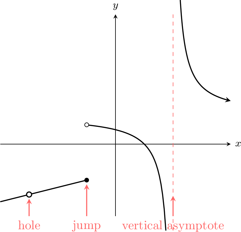
- Removable Discontinuity: Occurs when the limit exists but is not equal to the function's value, or the function is not defined at the point. This corresponds to a "hole" in the graph. It can be "removed" by redefining the function at that single point.
- Non-Removable (Essential) Discontinuity: Occurs when the limit does not exist. This corresponds to a "jump" (where one-sided limits differ), a vertical asymptote (an infinite discontinuity), or more complicated oscillatory behaviour.
Continuous Extension
A removable discontinuity can be repaired. If \(f\) is undefined at \(a\) but \(\displaystyle\lim_{x \to a} f(x) = L\) exists, the function \(\tilde{f}\) — defined on the domain of \(f\) together with \(a\), by \(\tilde{f}(x) = f(x)\) where \(f\) is defined and \(\tilde{f}(a) = L\) — is continuous at \(a\): it is called the continuous extension of \(f\) at \(a\). For instance, \(f(x) = \frac{x^2-1}{x-1}\) (undefined at \(1\)) extends into a continuous function by setting \(\tilde{f}(1) = 2\), since for \(x \neq 1\), \(\frac{x^2-1}{x-1} = x+1 \xrightarrow[x \to 1]{} 2\) — the hole is filled.
Proposition — A Catalog of Continuous Functions
The following types of functions are continuous at every number in their domains: - Polynomials (e.g., \(f(x)=x^2-3x+5\))
- Rational functions (e.g., \(f(x)=\dfrac{x+1}{x-2}\), continuous for \(x \neq 2\))
- Root functions (e.g., \(f(x)=\sqrt[n]{x}\), continuous on their domains)
- Trigonometric functions (e.g., \(\sin(x), \cos(x), \tan(x)\), etc., continuous on their domains)
- Inverse trigonometric functions (e.g., \(\arctan(x), \arcsin(x)\), etc.)
- Exponential functions (e.g., \(f(x)=e^x\))
- Natural logarithm (e.g., \(f(x)=\ln(x)\), continuous for \(x>0\))
Proposition — The Reference Continuous Functions
A short list of reference functions carries most of the work. Each of the following is continuous at every number of its domain: - Polynomial functions, and among them the affine functions and \(x \mapsto x^n\) (e.g. \(x \mapsto x^3 - 2x + 5\)), continuous on \(\mathbb{R}\);
- Rational functions (e.g. \(x \mapsto \dfrac{x+1}{x-2}\)), continuous on every interval where the denominator does not vanish;
- The square root function \(x \mapsto \sqrt{x}\), continuous on \([0\,;\,+\infty[\);
- The sine and cosine functions, continuous on \(\mathbb{R}\);
- The exponential function, continuous on \(\mathbb{R}\);
- The absolute value function \(x \mapsto |x|\), continuous on \(\mathbb{R}\).
Example
Let \(f\) be defined by $$f(x) = \begin{cases} x^2 + k & \text{if } x < 2, \\
3x - 1 & \text{if } x \geq 2. \end{cases}$$ Determine the value of \(k\) for which \(f\) is continuous at \(2\).
Each branch is a polynomial, hence continuous on its interval: only the join at \(x = 2\) is at stake.
- Left of the join: for \(x < 2\), \(f(x) = x^2 + k\), and \(x^2 + k \xrightarrow[x \to 2^-]{} 4 + k\).
- At the join and right of it: \(f(2) = 3 \times 2 - 1 = 5\), and \(3x - 1 \xrightarrow[x \to 2^+]{} 5\).
Skills to practice
- Reading Continuity on a Graph
- Studying Continuity at a Point
III
A Trigonometric Limit
III.1
The Limit of \(\sin\theta / \theta\)
Proposition — The Fundamental Trigonometric Limit
With \(\theta\) measured in radians, $$\lim_{\theta \to 0} \frac{\sin\theta}{\theta} = 1.$$ Example
Using the fundamental trigonometric limit, evaluate: - \(\displaystyle\lim_{x \to 0} \frac{\sin(3x)}{x}\);
- \(\displaystyle\lim_{\theta \to 0} \frac{\tan\theta}{\theta}\);
- \(\displaystyle\lim_{\theta \to 0} \frac{1-\cos\theta}{\theta}\).
- We make the pattern \(\frac{\sin u}{u}\) appear with \(u = 3x\): $$\frac{\sin(3x)}{x} = 3 \cdot \frac{\sin(3x)}{3x} \xrightarrow[x \to 0]{} 3 \times 1 = 3.$$
- Since \(\tan\theta = \dfrac{\sin\theta}{\cos\theta}\): $$\frac{\tan\theta}{\theta} = \frac{\sin\theta}{\theta} \cdot \frac{1}{\cos\theta} \xrightarrow[\theta \to 0]{} 1 \times \frac{1}{1} = 1.$$
- Multiplying by the conjugate \(1+\cos\theta\) and using \(1-\cos^2\theta = \sin^2\theta\): $$\frac{1-\cos\theta}{\theta} = \frac{\sin^2\theta}{\theta\,(1+\cos\theta)} = \frac{\sin\theta}{\theta} \cdot \frac{\sin\theta}{1+\cos\theta} \xrightarrow[\theta \to 0]{} 1 \times \frac{0}{2} = 0.$$
Skills to practice
- Evaluating Trigonometric Limits
IV
Limits of Sequences
IV.1
Convergence and Divergence
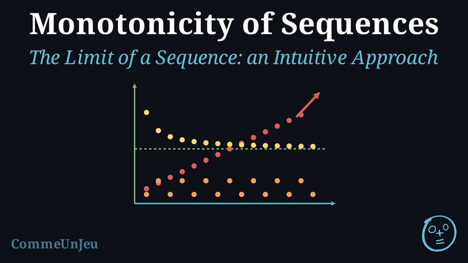
Once we know how a sequence varies, a second question arises: what happens to the terms \(u_n\) when \(n\) becomes very large — a thousand, a million, and beyond? Do they grow without bound, do they settle near a fixed number, or do they keep oscillating? This is the question of the limit of a sequence.
Definition — Limit of a Sequence
Let \((u_n)\) be a sequence. - \((u_n)\) has limit \(+\infty\) (as \(n\) tends to \(+\infty\)) if the terms \(u_n\) become as large as we want, provided \(n\) is large enough. We write \(\lim_{n \to +\infty} u_n = +\infty\).
- \((u_n)\) has limit \(-\infty\) if the terms \(u_n\) become as large negative as we want, provided \(n\) is large enough. We write \(\lim_{n \to +\infty} u_n = -\infty\).
- \((u_n)\) has limit a real number \(\ell\) if the terms \(u_n\) come as close to \(\ell\) as we want, provided \(n\) is large enough: we say that \((u_n)\) converges to \(\ell\), and we write \(\lim_{n \to +\infty} u_n = \ell\).
These ideas are first understood on examples: a table of values, a graph, a calculator or a short program let us conjecture the limit of a sequence. Proving that a conjectured limit is correct requires precise definitions of limits.
Example
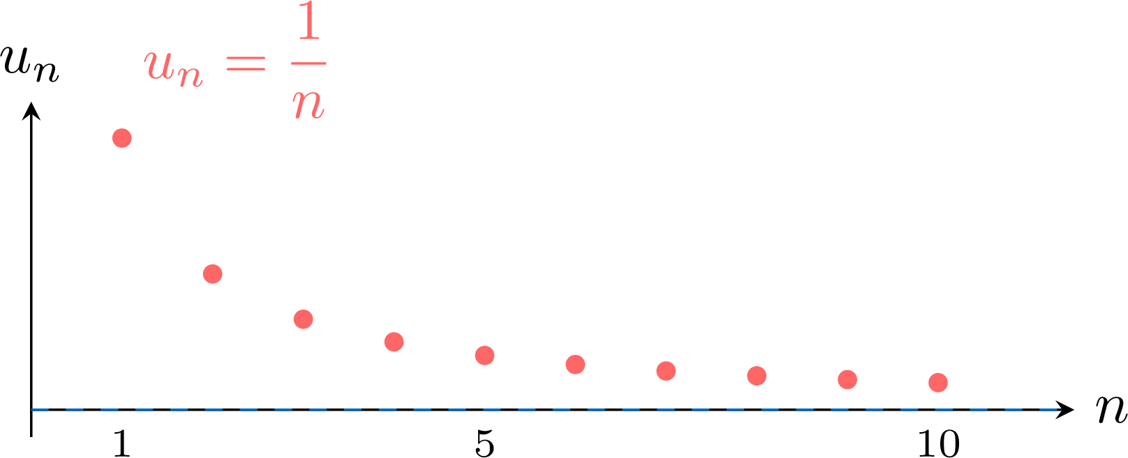
Conjecture the limit, if any, of each sequence defined for \(n \geq 1\): $$u_n = \frac{1}{n} \qquad v_n = n^2 \qquad w_n = (-1)^n \qquad t_n = 0.5^n$$
We compute a few terms for large values of \(n\):
| \(n\) | \(1\) | \(10\) | \(101\) | \(1000\) |
| \(u_n = 1/n\) | \(1\) | \(0.1\) | \(\approx 0.0099\) | \(0.001\) |
| \(v_n = n^2\) | \(1\) | \(100\) | \(10\,201\) | \(1\,000\,000\) |
| \(w_n = (-1)^n\) | \(-1\) | \(1\) | \(-1\) | \(1\) |
| \(t_n = 0.5^n\) | \(0.5\) | \(\approx 0.001\) | \(\approx 4 \times 10^{-31}\) | \(\approx 0\) |
- The terms \(u_n\) get as close to \(0\) as we want: we conjecture \(\lim u_n = 0\).
- The terms \(v_n\) become as large as we want: \(\lim v_n = +\infty\).
- \(w_n\) takes the values \(-1\) and \(1\) alternately (\(w_{101} = -1\)): no limit.
- The terms \(t_n\) get as close to \(0\) as we want: \(\lim t_n = 0\).
Skills to practice
- Conjecturing the Limit of a Sequence
IV.2
Limits of Geometric Sequences
Proposition — Limits of Geometric Sequences
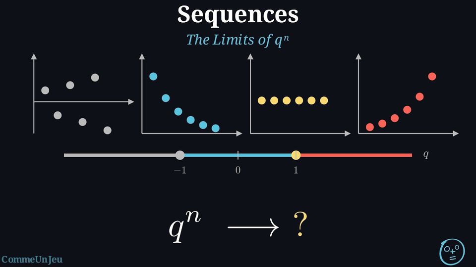
Let \(q\) be a real number. The limit of the sequence \((q^n)\) depends on the value of \(q\): - If \(\boldsymbol{q > 1}\), then \(\displaystyle \lim_{n \to +\infty} q^n = +\infty\).
- If \(\boldsymbol{-1 < q < 1}\), then \(\displaystyle \lim_{n \to +\infty} q^n = 0\).
- If \(\boldsymbol{q = 1}\), then the sequence is constant and \(\displaystyle \lim_{n \to +\infty} q^n = 1\).
- If \(\boldsymbol{q \le -1}\), then the sequence has no limit (it diverges).
Example
- \(\displaystyle \lim_{n \to +\infty} 1.05^n = +\infty\) because \(1.05 > 1\).
- \(\displaystyle \lim_{n \to +\infty} \left(\frac{1}{2}\right)^n = 0\) because \(-1 < 0.5 < 1\).
- The sequence \(((-2)^n)\) has no limit because \(-2 \le -1\).
Skills to practice
- Conjecturing the Limit of a Geometric Sequence
- Finding the Limit of a Geometric Sequence
V
Going further
Skills to practice
- Diagnosing Errors and Solving Problems
- Solving Problems with Technology
- Quiz
Jump to section