International Baccalaureate · DP 2: Analysis and Approaches HL

Applications of Differentiation

⌚ ~130 min ▢ 14 blocks ✓ 60 exercises ➣ Prerequisites : Properties of Curves, Introduction to Differential Calculus

I Optimisation

I.1 Optimising a Quadratic Function

Recappreviously studied — click to reread

Method — Optimising a Quadratic Function

Read the problem to identify the quantity to be maximised or minimised.
Define variables and write a quadratic function that models this quantity.
Find the coordinates of the vertex $(h,k)$ of the parabola.
- $h = -\frac{b}{2a}$ gives the input value (e.g., time, length, price) where the optimum occurs.
- $k = f(h)$ gives the optimal (maximum or minimum) value itself.
Check that $h$ is an allowed value of the variable (for instance, a length or a time is positive).
Answer the question in the context of the problem, making sure to include units.

Skills to practice

Optimising a Quadratic Function

I.2 Optimisation Problems

Optimisation is one of the most important applications of differential calculus. It involves finding the maximum or minimum value that a function can take, subject to given conditions. In many problems, this corresponds to finding the global maximum or minimum of that function on a specified domain.

Report an error

Definition — Optimisation

Optimisation is the process of finding a maximum or minimum value of a function, known as the objective function, subject to a set of constraints (or over a specified domain). The solution that achieves this is called the optimal solution.

Example

In machine learning, a key goal is to minimise a loss (error) function by adjusting model parameters. This optimisation process underlies how modern neural networks are trained.

Method — Solving Optimisation Problems

Model: Identify the quantity to be optimised and express it as a function of a single variable (for example $f(x)$). Use any given constraints to eliminate other variables. Determine the feasible domain for $x$.
Differentiate: Check that $f$ is differentiable on the domain, then find the first derivative of the function, $f'(x)$.
Find Stationary Points: Solve $f'(x)=0$ for $x$ in the domain.
Test and Justify: Use the sign of the derivative (sign table of $f'$, table of variations) to decide whether each stationary point is a local maximum, a local minimum, or neither.
Check Endpoints: If the domain is a closed interval $[a, b]$, evaluate the function at the stationary points and also at the endpoints, $f(a)$ and $f(b)$, to find the global extremum on that interval.
Conclusion: State the final answer clearly in the context of the problem, including units.

Example

A rectangle has a perimeter of 12 cm. Find its dimensions to maximise the area.

Answer

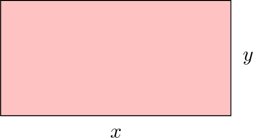
Model: Let the length be $x$ and the width be $y$. The perimeter is $2x+2y=12$, which simplifies to $x+y=6$ and hence $y=6-x$. The area is $A=xy$. We write $A$ as a function of $x$: $$ A(x) = x(6-x) = 6x-x^2. $$ Since lengths must be non-negative, $x \ge 0$ and $y=6-x \ge 0 \implies x \le 6$. The domain is $x \in [0,6]$.
Derivative: $$A'(x) = 6-2x.$$
Stationary point: $$ A'(x) = 0 \implies 6-2x=0 \implies 2x=6 \implies x=3. $$
Justification: sign of $A'$. $A'(x) = 6 - 2x$ is positive for $x < 3$ and negative for $x > 3$, so $A$ is increasing on $[0, 3]$ and decreasing on $[3, 6]$: $x = 3$ gives the maximum of $A$.
Check endpoints: The domain is the closed interval $[0,6]$. We check the area at the stationary point and at the endpoints, where $x = 0$ and $x = 6$ give flattened rectangles of area $0$:
- $A(0) = 6(0)-0^2 = 0$
- $A(3) = 6(3)-3^2 = 18-9 = 9$
- $A(6) = 6(6)-6^2 = 0$
The area is maximised at $x=3$.
Conclusion: The area is maximised when the length is $x=3$ cm. The corresponding width is $y=6-3=3$ cm. The rectangle with maximum area is therefore a square of side 3 cm, with an area of $9\text{ cm}^2$.

Example

A closed storage container with a square base must contain a volume of $8$ m$^3$. Find the dimensions that minimise the total surface area of the container.

Answer

Model: Let $x$ be the side of the square base and $h$ the height. The volume constraint gives $$x^2 h = 8 \implies h = \frac{8}{x^2}.$$ The surface consists of the base, the top and four lateral faces: $$S = 2x^2 + 4xh = 2x^2 + 4x \cdot \frac{8}{x^2} = 2x^2 + \frac{32}{x}.$$ The domain is $x \in (0, \infty)$ — an open interval: there are no endpoints to check, so the justification must come from the variations.
Derivative: $$S'(x) = 4x - \frac{32}{x^2} = \frac{4x^3 - 32}{x^2}.$$
Stationary point: $S'(x) = 0 \iff 4x^3 = 32 \iff x^3 = 8 \iff x = 2$.
Test and justify: the sign of $S'(x)$ is the sign of $4x^3 - 32$: negative for $0 < x < 2$, positive for $x > 2$. So $S$ decreases on $(0, 2]$ and increases on $[2, \infty)$: the variation table shows that $x = 2$ gives the global minimum on the whole domain — no endpoint check is possible, and none is needed.
Conclusion: $x = 2$ m and $h = \frac{8}{4} = 2$ m: the optimal container is a cube of side $2$ m, with total surface $S(2) = 2(4) + \frac{32}{2} = 24$ m$^2$.

Skills to practice

Setting Up an Optimisation Problem
Solving Optimisation Problems
Solving Optimisation Problems in Context

I.3 An Optimum at an End Point

Example

A wire $20$ cm long is cut into two pieces. A piece of length $x$ cm is bent into a square, and the other piece into a circle. The values $x = 0$ and $x = 20$ mean that the whole wire makes a single shape, so $0 \le x \le 20$.

Show that the total area enclosed is $A(x) = \dfrac{x^2}{16} + \dfrac{(20 - x)^2}{4\pi}$ cm$^2$.
Find the value of $x$ for which $A'(x) = 0$, and show that it gives the least total area.
Where should the wire be cut to enclose the greatest total area?

Answer

The square has perimeter $x$, so its side is $\dfrac{x}{4}$ and its area $\dfrac{x^2}{16}$. The circle has circumference $2\pi\rho = 20 - x$, so its radius is $\rho = \dfrac{20 - x}{2\pi}$ and its area is $$\begin{aligned}[t] \pi\rho^2 &= \pi \times \frac{(20 - x)^2}{4\pi^2} && \text{(area of a disc, } \rho = \tfrac{20 - x}{2\pi}\text{)} \\ &= \frac{(20 - x)^2}{4\pi}. \end{aligned}$$ Adding the two areas gives $A(x) = \dfrac{x^2}{16} + \dfrac{(20 - x)^2}{4\pi}$.
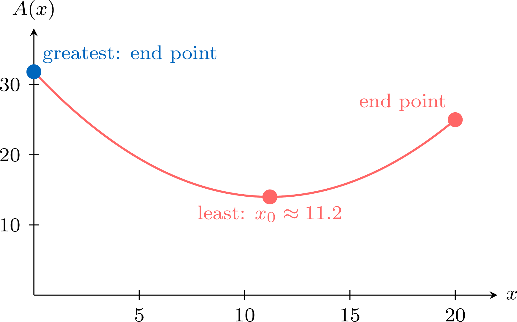
Since $(20 - x)^2 = 400 - 40x + x^2$ has derivative $-40 + 2x = -2(20 - x)$, $$\begin{aligned}[t] A'(x) &= \frac{2x}{16} - \frac{2(20 - x)}{4\pi} && \text{(power rule, term by term)} \\ &= \frac{x}{8} - \frac{20 - x}{2\pi} \\ &= \frac{\pi x - 4(20 - x)}{8\pi} && \text{(common denominator } 8\pi\text{)} \\ &= \frac{(\pi + 4)x - 80}{8\pi}. \end{aligned}$$ So $A'(x) = 0$ for $x_0 = \dfrac{80}{\pi + 4} \approx 11.2$. Since $8\pi > 0$ and $\pi + 4 > 0$, $A'(x)$ has the sign of $(\pi + 4)x - 80$: negative for $x < x_0$, positive for $x > x_0$. 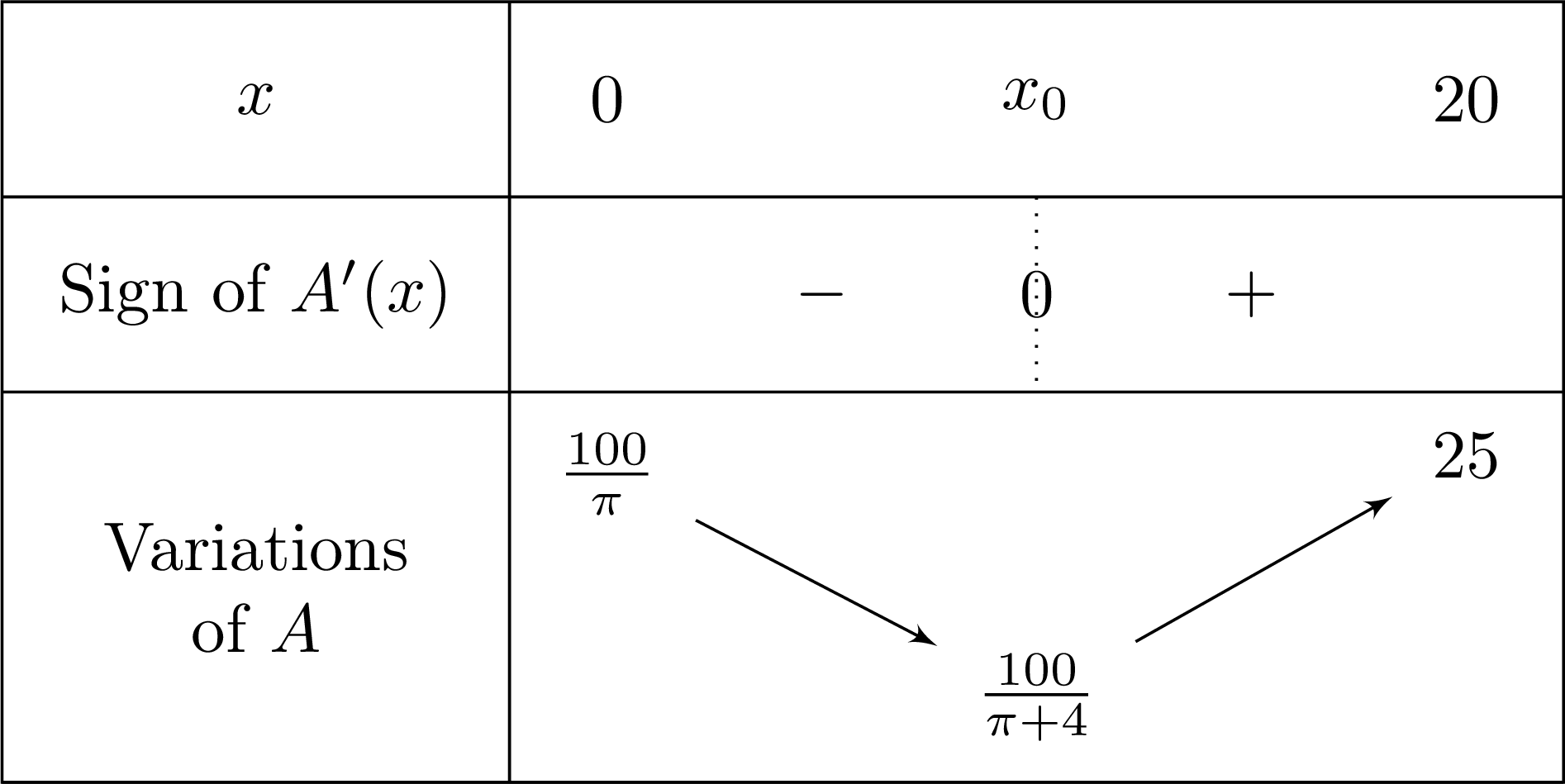$A$ decreases, then increases: $x_0$ gives the least total area. With $\dfrac{x_0}{4} = \dfrac{20}{\pi + 4}$ and $20 - x_0 = \dfrac{20\pi}{\pi + 4}$, $$\begin{aligned}[t] A(x_0) &= \frac{400}{(\pi + 4)^2} + \frac{400\pi^2}{4\pi(\pi + 4)^2} \\ &= \frac{400 + 100\pi}{(\pi + 4)^2} \\ &= \frac{100}{\pi + 4} \approx 14.0 \text{ cm}^2. \end{aligned}$$
The only stationary point is a minimum: the greatest value of $A$ on $[0, 20]$ is at an end point. Compare the values at the end points: $$A(0) = \frac{400}{4\pi} = \frac{100}{\pi} \approx 31.8 \qquad \text{and} \qquad A(20) = \frac{400}{16} = 25.$$ Since $\pi < 4$, $\dfrac{100}{\pi} > \dfrac{100}{4} = 25$. The greatest total area, $\dfrac{100}{\pi} \approx 31.8$ cm$^2$, is reached for $x = 0$: the wire is not cut, and all of it is bent into a circle.

Setting $A'(x) = 0$ found the worst cut, not the best one: on a closed interval, the values at the end points are always compared with the values at the stationary points (step 5 of the Method).

Skills to practice

Finding an Optimum at an End Point

I.4 Optimisation with Technology

Example

An oil platform $P$ stands $4$ km off a straight coast; $A$ is the point of the coast nearest to $P$, and a refinery $R$ stands on the coast, $10$ km from $A$. A pipeline runs straight under the sea from $P$ to a point $M$ of the coast between $A$ and $R$, with $AM = x$ km, then along the coast from $M$ to $R$. Laying the pipeline costs $5$ million dollars per km under the sea and $3$ million dollars per km on land.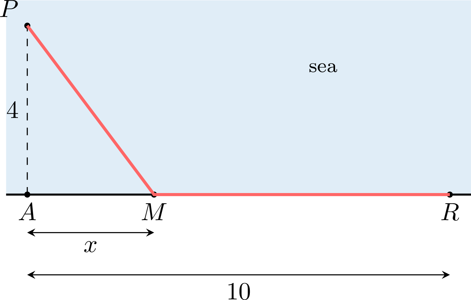

Show that the total cost, in millions of dollars, is $C(x) = 5\sqrt{16 + x^2} + 3(10 - x)$, for $0 \le x \le 10$.
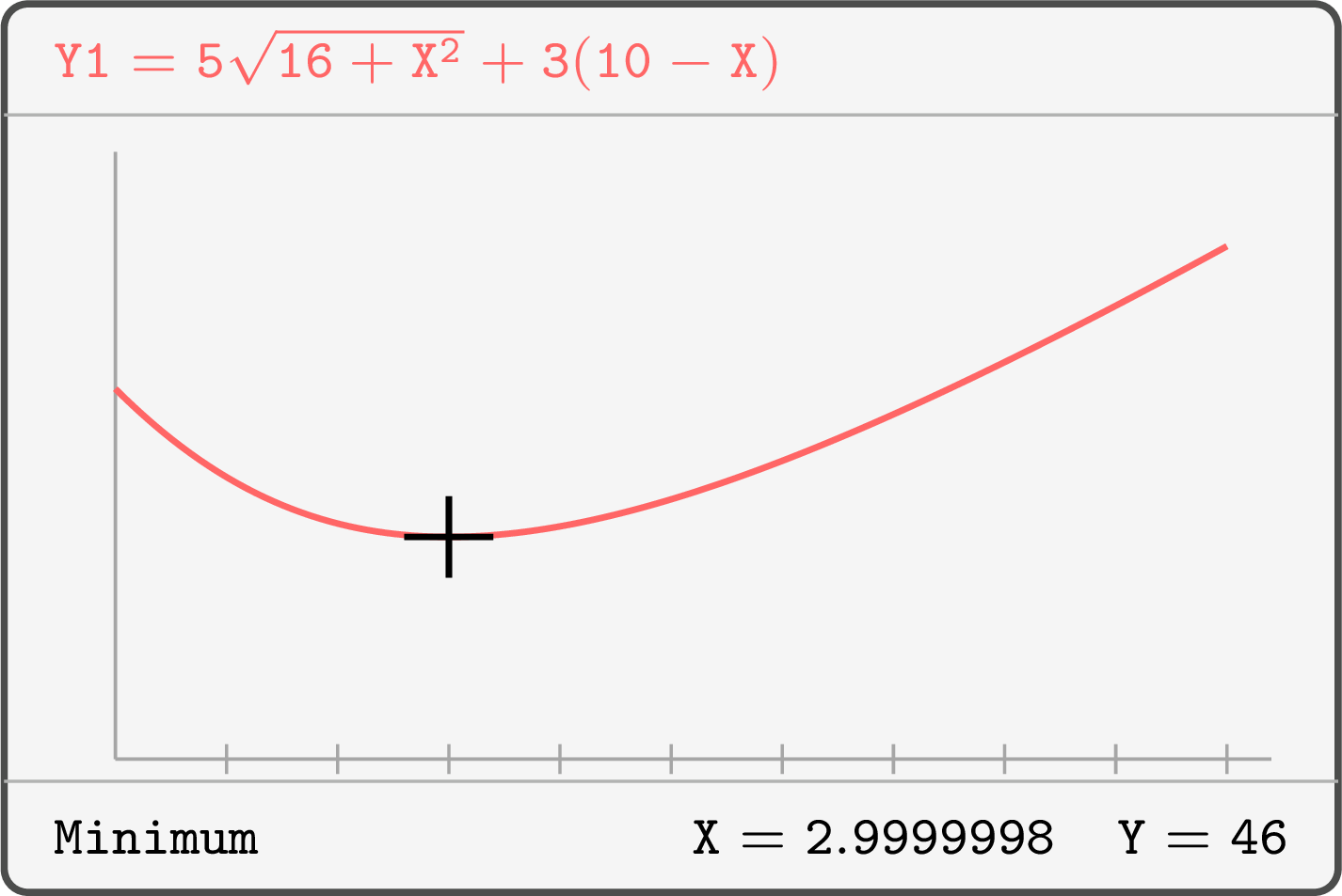
Use technology to find where the pipeline should reach the coast, and the least cost.

Answer

The triangle $PAM$ is right-angled at $A$, so by Pythagoras' theorem $PM = \sqrt{AP^2 + AM^2} = \sqrt{16 + x^2}$ km, and $MR = 10 - x$ km. The cost is $5$ times the length under the sea plus $3$ times the length on land: $$C(x) = 5\sqrt{16 + x^2} + 3(10 - x), \qquad 0 \le x \le 10.$$
Enter $Y_1 = 5\sqrt{16 + X^2} + 3(10 - X)$ with the window $0 \le x \le 10$, $40 \le y \le 56$. The curve falls, then rises: the minimum tool, with bounds on either side of the lowest point, displays $X \approx 3$ and $Y \approx 46$ (a value such as $X = 2.9999998$ is the tool's approximation: the tool finds the minimum to its precision, not exactly). The values at the end points are larger: $C(0) = 5 \times 4 + 30 = 50$ and $C(10) = 5\sqrt{116} \approx 53.9$. The pipeline should reach the coast about $3$ km from $A$, that is about $7$ km before the refinery, for a least cost of about $46$ million dollars. A table of values agrees with the reading: $C(3) = 5\sqrt{25} + 21 = 46$, while $C(2.9) \approx 46.003$ and $C(3.1) \approx 46.003$ are slightly larger.

The curve is very flat near its lowest point: the table of values gives $C(2.5) \approx 46.08$ and $C(3.5) \approx 46.08$, so landing the pipeline half a kilometre on either side of the best point costs less than $0.1$ million dollars more. Zooming in on the graph, or reading a table, shows how sensitive the cost is to the choice of $x$ — information that the single optimal value does not give.

Skills to practice

Solving Optimisation Problems with Technology

II Rates of Change

II.1 Rates of Change with Respect to Time

When a quantity $Q$ depends on the time $t$, the derivative $Q'(t) = \dfrac{\mathrm{d}Q}{\mathrm{d}t}(t)$ is the instantaneous rate of change of $Q$: how fast $Q$ changes at the instant $t$, the value approached by the average rate $\dfrac{\Delta Q}{\Delta t}$ over shorter and shorter durations. Its unit is the unit of $Q$ divided by the unit of time. Speed is the best-known example; physics and chemistry give two more.

Power: if $E(t)$ is the energy received by a system from the instant $0$ to the instant $t$, the power at the instant $t$ is $P(t) = \dfrac{\mathrm{d}E}{\mathrm{d}t}(t)$, in watts ($\mathrm{W}$) when $E$ is in joules ($\mathrm{J}$) and $t$ in seconds. When the power is constant, the energy received during a duration $\Delta t$ is $\Delta E = P \times \Delta t$.
Reaction rates: during a chemical reaction, the concentration $[A](t)$ of a reactant $A$ decreases, and its rate of disappearance is $-\dfrac{\mathrm{d}[A]}{\mathrm{d}t}(t)$, which is non-negative; the concentration $[B](t)$ of a product $B$ increases, and its rate of appearance is $\dfrac{\mathrm{d}[B]}{\mathrm{d}t}(t)$. With concentrations in $\mathrm{mol \cdot L^{-1}}$ and $t$ in minutes, these rates are in $\mathrm{mol \cdot L^{-1} \cdot min^{-1}}$.

Report an error

Example

During a test, the energy received by a water heater from the instant $0$ to the instant $t$ is $E(t) = 2t^2 + 10t$, in joules, for $0 \leq t \leq 10$ ($t$ in seconds).

Compute the power $P(t)$, then $P(0)$ and $P(10)$.
Compute the average power over the test, $\dfrac{E(10) - E(0)}{10 - 0}$, and compare it with $P(0)$ and $P(10)$.

Answer

$$\begin{aligned}[t] P(t) &= E'(t) &&\text{(the power is the derivative of the energy)}\\ &= 2 \times 2t + 10 &&\text{(} (t^2)' = 2t\text{, } (t)' = 1\text{)}\\ &= 4t + 10.\end{aligned}$$ The expression of $E$ is a polynomial, differentiable at every real $t$, including $t = 0$ and $t = 10$. So $P(0) = 10~\mathrm{W}$ and $P(10) = 50~\mathrm{W}$: the power grows during the test.
$E(10) = 200 + 100 = 300~\mathrm{J}$ and $E(0) = 0$, so the average power is $\dfrac{300}{10} = 30~\mathrm{W}$, between $P(0) = 10~\mathrm{W}$ and $P(10) = 50~\mathrm{W}$. A constant power of $30~\mathrm{W}$ would give the same energy: $30 \times 10 = 300~\mathrm{J}$.

Example

In a reaction $A \to B$, the concentration of the reactant $A$, in $\mathrm{mol \cdot L^{-1}}$, is $[A](t) = \dfrac{0.5}{1 + 0.1t}$ for $t \geq 0$ ($t$ in minutes). Each mole of $A$ that disappears gives one mole of $B$, and there is no $B$ at the start, so $[B](t) = 0.5 - [A](t)$.

Compute the rate of disappearance of $A$ at $t = 0$ and at $t = 10$.
Show that the rate of appearance of $B$ is equal to the rate of disappearance of $A$.

Answer

$$\begin{aligned}[t]\frac{\mathrm{d}[A]}{\mathrm{d}t}(t) &= \frac{0 \times (1 + 0.1t) - 0.5 \times 0.1}{(1 + 0.1t)^2} &&\text{(quotient rule)}\\ &= -\frac{0.05}{(1 + 0.1t)^2}.\end{aligned}$$ The rate of disappearance is $r(t) = \dfrac{0.05}{(1 + 0.1t)^2}$: $r(0) = 0.05~\mathrm{mol \cdot L^{-1} \cdot min^{-1}}$ and $r(10) = \dfrac{0.05}{2^2} = 0.0125~\mathrm{mol \cdot L^{-1} \cdot min^{-1}}$. The reaction slows down as the reactant is used up.
$\dfrac{\mathrm{d}[B]}{\mathrm{d}t}(t) = 0 - \dfrac{\mathrm{d}[A]}{\mathrm{d}t}(t) = r(t)$: $B$ appears exactly as fast as $A$ disappears.

Skills to practice

Interpreting a Rate of Change
Computing a Rate of Change in Context
Modelling with Rates of Change

II.2 Related Rates

In many real-world situations, several quantities vary with time, and their rates of change are related. For example, the volume, radius, and surface area of a growing spherical balloon are all functions of time, and their rates of change are connected. Related rates problems involve finding the rate of change of one quantity by relating it to other quantities whose rates of change are known.

Report an error

Method — Solving Related Rates Problems

Model: Identify all quantities that are changing with time and assign them variables. Write down the given rates of change and the rate to be found (at a specific instant).
Equation: Find an equation that relates the variables.
Differentiate: Differentiate both sides of the equation with respect to time ($t$), using the chain rule.
Substitute and Solve: Substitute all known values (including the value of each variable at the instant of interest) into the differentiated equation and solve for the unknown rate.

Example

Air is being pumped into a spherical balloon so that its volume increases at a rate of 100 cm$^3$/s. How fast is the radius of the balloon increasing when the diameter is 50 cm?

Answer

Model: Let $V$ be the volume and $r$ be the radius of the balloon. We are given the rate of change of the volume: $$\dfrac{\mathrm{d}V}{\mathrm{d}t} = 100\ \text{cm}^3/\text{s}.$$ We want to find the rate of change of the radius, $\dfrac{\mathrm{d}r}{\mathrm{d}t}$, at the instant when the diameter is 50 cm, which means the radius is $r = 25$ cm.
Equation: The volume of a sphere is given by the formula $$V = \frac{4}{3}\pi r^3.$$
Differentiate: We differentiate both sides with respect to time $t$: $$ \frac{d}{\mathrm{d}t}(V) = \frac{d}{\mathrm{d}t}\left(\frac{4}{3}\pi r^3\right). $$ Using the chain rule on the right side: $$ \frac{\mathrm{d}V}{\mathrm{d}t} = \frac{4}{3}\pi \cdot (3r^2) \cdot \frac{\mathrm{d}r}{\mathrm{d}t} = 4\pi r^2 \frac{\mathrm{d}r}{\mathrm{d}t}. $$
Substitute and solve: Now, we substitute the known values into this equation: $$ 100 = 4\pi (25)^2 \frac{\mathrm{d}r}{\mathrm{d}t} $$ $$ 100 = 4\pi(625) \frac{\mathrm{d}r}{\mathrm{d}t} $$ $$ 100 = 2500\pi \frac{\mathrm{d}r}{\mathrm{d}t}. $$ Solving for $\dfrac{\mathrm{d}r}{\mathrm{d}t}$: $$ \frac{\mathrm{d}r}{\mathrm{d}t} = \frac{100}{2500\pi} = \frac{1}{25\pi}. $$
Conclusion: The radius of the balloon is increasing at a rate of $$\dfrac{1}{25\pi}\ \text{cm/s}$$ when the diameter is 50 cm.

Example

Two cars leave the same intersection at noon. Car A drives east at $60$ km/h and car B drives north at $80$ km/h. How fast is the distance between the two cars increasing at 12:30?

Answer

Model: at time $t$ (in hours after noon), let $x$ be the distance driven by A, $y$ the distance driven by B, and $z$ the distance between the cars. We know $\dfrac{\mathrm{d}x}{\mathrm{d}t} = 60$ and $\dfrac{\mathrm{d}y}{\mathrm{d}t} = 80$, and we want $\dfrac{\mathrm{d}z}{\mathrm{d}t}$ at $t = \dfrac12$.
Equation: the roads are perpendicular, so by the Pythagorean theorem $$z^2 = x^2 + y^2.$$ Working with $z^2$ instead of $z = \sqrt{x^2+y^2}$ avoids differentiating a square root.
Differentiate — before substituting any instant values, since $x$, $y$, $z$ all vary: $$2z\frac{\mathrm{d}z}{\mathrm{d}t} = 2x\frac{\mathrm{d}x}{\mathrm{d}t} + 2y\frac{\mathrm{d}y}{\mathrm{d}t}, \qquad \text{so} \qquad z\frac{\mathrm{d}z}{\mathrm{d}t} = x\frac{\mathrm{d}x}{\mathrm{d}t} + y\frac{\mathrm{d}y}{\mathrm{d}t}.$$
Substitute and solve: at $t = \frac12$: $x = 30$ km, $y = 40$ km, and $z = \sqrt{30^2 + 40^2} = 50$ km. Then $$\frac{\mathrm{d}z}{\mathrm{d}t} = \frac{30 \times 60 + 40 \times 80}{50} = \frac{1800 + 3200}{50} = \frac{5000}{50} = 100.$$
Conclusion: at 12:30 the distance between the cars is increasing at $100$ km/h — faster than either car drives, because both motions push the cars apart.

Skills to practice

Setting Up Related Rates
Computing Related Rates
Solving Related Rates Problems

III Going further

Skills to practice

Diagnosing and Correcting Errors
Solving Exam-Style Problems on Optimisation and Rates of Change
Quiz