French National Education · ECGapprofondies 2

Linear algebra complements

⌚ ~91 min ▢ 11 blocks ✓ 46 exercises PDFFull lesson PDFExercise sheet PDFSolutions ➣ Prerequisites : Vector spaces of finite dimension, Linear maps, Matrices

This course extends three pillars of linear algebra established in the previous course. First, the notion of direct sum, met for two subspaces, is generalised to an arbitrary finite family of subspaces, together with the language of adapted bases. Second, the change-of-basis machinery for vectors is extended to endomorphisms: the matrix of one endomorphism in two different bases is governed by the formula $\mathrm{Mat}_{B'}(f) = P_{B, B'}^{-1}\, \mathrm{Mat}_B(f)\, P_{B, B'}$, which leads to the relation of similar matrices. Third, the trace of a square matrix is introduced as the simplest invariant attached to a matrix; together with the rank, it provides the practical toolkit for distinguishing classes of similar matrices. These three pillars form the algebraic toolbox used in the next course to study eigenvalues and reduction of endomorphisms. Convention: throughout this course $E$ denotes a real vector space of finite dimension, except when stated otherwise; all matrices have real entries, and $K = \mathbb{R}$ is implicit.

I Direct sums of subspaces

We have already studied, for two subspaces $F$ and $G$ of $E$, the sum $F + G$ and the direct sum $F \oplus G$, together with the criterion $F \cap G = \{0_E\}$ and the dimension formula $\dim(F + G) = \dim F + \dim G - \dim(F \cap G)$. We now extend these notions to a family of $k$ subspaces $F_1, \dots, F_k$, with $k \ge 2$. The generalisation is largely formal, but it brings two new ideas: the adapted basis, which records the decomposition $E = F_1 \oplus \dots \oplus F_k$ at the level of vectors, and a subtle warning for $k \ge 3$ that the pairwise criterion $F_i \cap F_j = \{0_E\}$ is not sufficient to ensure that the sum is direct.

I.1 Sum and direct sum of $k$ subspaces

The sum of $k$ subspaces collects all vectors that can be written as $x_1 + \dots + x_k$ with $x_i \in F_i$. The sum is called direct when this decomposition is unique. The new content of this subsection is the criterion phrased on the zero vector, which replaces the two-subspace test $F \cap G = \{0_E\}$.

Definition — Sum of $k$ subspaces

Let $F_1, \dots, F_k$ be subspaces of $E$. The sum of $F_1, \dots, F_k$, written $F_1 + \dots + F_k$ or $\sum_{i = 1}^k F_i$, is the set $$ F_1 + \dots + F_k = \bigl\{ x_1 + \dots + x_k \,:\, x_i \in F_i \text{ for every } i \in \{1, \dots, k\} \bigr\}. $$

Example

In $\mathbb{R}^3$ with canonical basis $(e_1, e_2, e_3)$, set $F_i = \mathrm{Vect}(e_i)$ for $i \in \{1, 2, 3\}$. Then $F_1 + F_2 + F_3 = \mathbb{R}^3$: every vector $(x_1, x_2, x_3)$ writes $x_1 e_1 + x_2 e_2 + x_3 e_3$ with $x_i e_i \in F_i$.

Example

In $\mathbb{R}_3[X]$, set $F_0 = \mathrm{Vect}(1)$, $F_1 = \mathrm{Vect}(X)$, $F_2 = \mathrm{Vect}(X^2)$, $F_3 = \mathrm{Vect}(X^3)$. Then $F_0 + F_1 + F_2 + F_3 = \mathbb{R}_3[X]$: every polynomial of degree at most $3$ writes $a_0 \cdot 1 + a_1 X + a_2 X^2 + a_3 X^3$ with each $a_i \cdot X^i \in F_i$.

Proposition — The sum is a subspace

Let $F_1, \dots, F_k$ be subspaces of $E$. Then $F_1 + \dots + F_k$ is a subspace of $E$.

Proof

The zero vector $0_E = 0_E + \dots + 0_E$ belongs to the sum since each $0_E \in F_i$. Let $x = \sum_{i = 1}^k x_i$ and $y = \sum_{i = 1}^k y_i$ with $x_i, y_i \in F_i$, and let $\lambda, \mu \in \mathbb{R}$. Then $$ \begin{aligned} \lambda x + \mu y &= \lambda \sum_{i = 1}^k x_i + \mu \sum_{i = 1}^k y_i && \text{(definition of } x \text{ and } y\text{)} \\ &= \sum_{i = 1}^k (\lambda x_i + \mu y_i) && \text{(linearity of the sum)}, \end{aligned} $$ and each $\lambda x_i + \mu y_i$ lies in $F_i$ because $F_i$ is a subspace. Hence $\lambda x + \mu y \in F_1 + \dots + F_k$, which is therefore a subspace of $E$.

Definition — Direct sum of $k$ subspaces

The sum $F_1 + \dots + F_k$ is said to be direct when, for every $x \in F_1 + \dots + F_k$, there exists a unique $k$-tuple $(x_1, \dots, x_k) \in F_1 \times \dots \times F_k$ such that $x = x_1 + \dots + x_k$. In that case, the sum is written $$ F_1 \oplus \dots \oplus F_k \quad \text{or} \quad \bigoplus_{i = 1}^k F_i. $$

Example

In $\mathbb{R}^3$, the sum $\mathrm{Vect}(e_1) + \mathrm{Vect}(e_2) + \mathrm{Vect}(e_3)$ is direct: every $(x_1, x_2, x_3)$ writes uniquely $x_1 e_1 + x_2 e_2 + x_3 e_3$. So $\mathbb{R}^3 = \mathrm{Vect}(e_1) \oplus \mathrm{Vect}(e_2) \oplus \mathrm{Vect}(e_3)$.

Example — Symmetric and antisymmetric matrices

Recall the symmetric and antisymmetric subspaces of $\mathcal{M}_n(\mathbb{R})$: $$ \mathcal{S}_n(\mathbb{R}) = \{ A \in \mathcal{M}_n(\mathbb{R}) \,:\, {}^t A = A \}, \qquad \mathcal{A}_n(\mathbb{R}) = \{ A \in \mathcal{M}_n(\mathbb{R}) \,:\, {}^t A = -A \}. $$ Every matrix $A \in \mathcal{M}_n(\mathbb{R})$ decomposes as $$ A = \underbrace{\frac{1}{2}\bigl(A + {}^t A\bigr)}_{\in\, \mathcal{S}_n(\mathbb{R})} \;+\; \underbrace{\frac{1}{2}\bigl(A - {}^t A\bigr)}_{\in\, \mathcal{A}_n(\mathbb{R})}, $$ and the two components are unique: if $A = S + T$ with $S$ symmetric and $T$ antisymmetric, then transposing gives ${}^t A = S - T$, hence $S = \frac{1}{2}(A + {}^t A)$ and $T = \frac{1}{2}(A - {}^t A)$. Therefore $\mathcal{M}_n(\mathbb{R}) = \mathcal{S}_n(\mathbb{R}) \oplus \mathcal{A}_n(\mathbb{R})$.

Proposition — Characterisation of a direct sum

The sum $F_1 + \dots + F_k$ is direct if and only if the only decomposition of the zero vector is the trivial one: $$ \bigl( \forall (x_1, \dots, x_k) \in F_1 \times \dots \times F_k, \quad x_1 + \dots + x_k = 0_E \;\Rightarrow\; \forall i, \ x_i = 0_E \bigr). $$

Proof

We prove both implications.

Direct $\Rightarrow$ trivial zero-decomposition. Suppose the sum is direct. Take $(x_1, \dots, x_k)$ with $x_1 + \dots + x_k = 0_E$. Since $0_E$ also writes as $0_E + \dots + 0_E$ with $0_E \in F_i$, uniqueness of the decomposition of $0_E$ forces $x_i = 0_E$ for every $i$.
Trivial zero-decomposition $\Rightarrow$ direct. Suppose the zero-decomposition is trivial. Let $x \in F_1 + \dots + F_k$ admit two decompositions $x = x_1 + \dots + x_k = y_1 + \dots + y_k$ with $x_i, y_i \in F_i$. Then $$ \begin{aligned} (x_1 - y_1) + \dots + (x_k - y_k) &= x - x = 0_E && \text{(subtracting the two decompositions)}, \end{aligned} $$ and each $x_i - y_i \in F_i$. The trivial-zero-decomposition hypothesis gives $x_i - y_i = 0_E$, that is $x_i = y_i$, for every $i$. The decomposition of $x$ is therefore unique, and the sum is direct.

Pairwise-intersection trap for $k \ge 3$

For two subspaces, the criterion $F \cap G = \{0_E\}$ is equivalent to $F + G$ being direct. This equivalence breaks down for $k \ge 3$: the condition $F_i \cap F_j = \{0_E\}$ for every $i \ne j$ does not suffice to ensure that $F_1 + \dots + F_k$ is direct. The correct criterion is the zero-decomposition condition above; it must be checked on all indices simultaneously, not pair by pair.

Example — Counter-example to the pairwise criterion

In $\mathbb{R}^2$ with canonical basis $(e_1, e_2)$, set $$ F = \mathrm{Vect}(e_1), \qquad G = \mathrm{Vect}(e_2), \qquad H = \mathrm{Vect}(e_1 + e_2). $$ Each pair of subspaces intersects trivially: $F \cap G = \{0\}$, $F \cap H = \{0\}$, $G \cap H = \{0\}$ (any non-zero vector of $F$ has zero second coordinate, while any non-zero vector of $H$ has equal coordinates, so the only common vector is $0$; symmetrically for the other pairs). Yet the sum $F + G + H$ is not direct: the vector $e_1 + e_2$ has two distinct decompositions, $$ \begin{aligned} e_1 + e_2 &= e_1 + e_2 + 0 && \text{(decomposition in } F + G + H \text{ via } F \text{ and } G\text{)}, \\ e_1 + e_2 &= 0 + 0 + (e_1 + e_2) && \text{(decomposition via } H\text{)}. \end{aligned} $$ The hypothesis $F_i \cap F_j = \{0\}$ is therefore not strong enough for $k \ge 3$.

Method — Showing that a sum is direct

To prove that the sum $F_1 + \dots + F_k$ is direct:

Take an arbitrary $k$-tuple $(x_1, \dots, x_k) \in F_1 \times \dots \times F_k$ such that $x_1 + \dots + x_k = 0_E$.
Show that this implies $x_i = 0_E$ for every $i \in \{1, \dots, k\}$ (use the explicit description of each $F_i$).
Conclude using the characterisation above.

Warning. For $k \ge 3$, do not use the pairwise criterion $F_i \cap F_j = \{0_E\}$: it does not imply that the sum is direct. The zero-decomposition criterion above is the recommended one; an equivalent test using basis concatenation will appear in the next subsection.

Skills to practice

Showing a sum is direct
Identifying a direct sum from a basis

I.2 Adapted basis and basis concatenation

When $E = F_1 \oplus \dots \oplus F_k$, the direct-sum structure can be lifted from vectors to bases: by picking a basis $\mathcal{B}_i$ in each $F_i$ and concatenating them, we obtain a basis of $E$ that respects the decomposition. Such a basis is called adapted, and the operation gives us at once an explicit method to compute the dimension of a direct sum.

Definition — Adapted basis to a direct sum

Suppose $E = F_1 \oplus \dots \oplus F_k$. Let $\mathcal{B}_i$ be a basis of $F_i$ for each $i$. The family of $E$ obtained by concatenating $\mathcal{B}_1, \dots, \mathcal{B}_k$ in order, $$ \mathcal{B} = \mathcal{B}_1 \sqcup \mathcal{B}_2 \sqcup \dots \sqcup \mathcal{B}_k, $$ is called a family adapted to the direct-sum decomposition $E = F_1 \oplus \dots \oplus F_k$. (The theorem below shows that this concatenation is in fact a basis of $E$, hence the common name adapted basis.)

Example

The canonical basis $(e_1, \dots, e_n)$ of $\mathbb{R}^n$ is adapted to the direct-sum decomposition $$ \mathbb{R}^n = \mathrm{Vect}(e_1) \oplus \mathrm{Vect}(e_2) \oplus \dots \oplus \mathrm{Vect}(e_n). $$ Each $\mathcal{B}_i = (e_i)$ is a basis of the line $\mathrm{Vect}(e_i)$, and their concatenation is exactly the canonical basis.

Example

In $\mathbb{R}^3$, set $F = \mathrm{Vect}(e_1, e_2)$ (the horizontal plane) and $G = \mathrm{Vect}(e_3)$ (the vertical line). The direct sum decomposes as $\mathbb{R}^3 = F \oplus G$ (every vector $(x, y, z)$ writes uniquely $(x, y, 0) + (0, 0, z)$). A basis of $F$ is $(e_1, e_2)$, a basis of $G$ is $(e_3)$, and the concatenation is the canonical basis $(e_1, e_2, e_3)$: an adapted basis. Replacing $G$ by $G' = \mathrm{Vect}(e_1 + e_2 + e_3)$ also yields a direct-sum decomposition $\mathbb{R}^3 = F \oplus G'$, and the corresponding adapted basis is $(e_1, e_2, e_1 + e_2 + e_3)$.

Proposition — Concatenation generates the sum

Let $F_1, \dots, F_k$ be subspaces of $E$, and let $\mathcal{B}_i$ be a basis of $F_i$ for each $i$. Then the concatenation $\mathcal{B}_1 \sqcup \dots \sqcup \mathcal{B}_k$ is a generating family of $F_1 + \dots + F_k$.
This holds regardless of whether the sum is direct or not.

Proof

Let $x \in F_1 + \dots + F_k$. By definition there exist $x_i \in F_i$ such that $x = x_1 + \dots + x_k$. Since $\mathcal{B}_i$ generates $F_i$, each $x_i$ is a linear combination of the vectors of $\mathcal{B}_i$. Summing these linear combinations across $i$, $x$ is itself a linear combination of the vectors of the concatenation $\mathcal{B}_1 \sqcup \dots \sqcup \mathcal{B}_k$, which therefore generates $F_1 + \dots + F_k$.

Theorem — Characterisation of a direct sum by basis concatenation

Let $F_1, \dots, F_k$ be subspaces of $E$, and let $\mathcal{B}_i$ be a basis of $F_i$ for each $i$. The following statements are equivalent:

the sum $F_1 + \dots + F_k$ is direct;
the concatenation $\mathcal{B}_1 \sqcup \dots \sqcup \mathcal{B}_k$ is a linearly independent family of $E$;
the concatenation $\mathcal{B}_1 \sqcup \dots \sqcup \mathcal{B}_k$ is a basis of $F_1 + \dots + F_k$.

Proof

Write $\mathcal{B}_i = (b_{i, 1}, \dots, b_{i, p_i})$, where $p_i = \dim F_i$.

(1) $\Rightarrow$ (2). Suppose the sum is direct. A linear combination $\sum_{i = 1}^k \sum_{j = 1}^{p_i} \lambda_{i, j}\, b_{i, j} = 0_E$ can be rewritten $\sum_{i = 1}^k x_i = 0_E$ with $x_i = \sum_{j = 1}^{p_i} \lambda_{i, j}\, b_{i, j} \in F_i$. The previous characterisation of direct sums forces $x_i = 0_E$ for every $i$. Since $\mathcal{B}_i$ is a basis, hence linearly independent, all $\lambda_{i, j} = 0$. The concatenation is therefore linearly independent.
(2) $\Rightarrow$ (3). Suppose the concatenation is linearly independent. The previous Proposition shows that it also generates $F_1 + \dots + F_k$. A family that is both linearly independent and generating is a basis.
(3) $\Rightarrow$ (1). Suppose the concatenation is a basis of $F_1 + \dots + F_k$. Take a zero-decomposition $\sum_{i = 1}^k x_i = 0_E$ with $x_i \in F_i$. Writing each $x_i$ in the basis $\mathcal{B}_i$ gives a linear combination of the concatenation equal to $0_E$, hence all coordinates vanish. Therefore each $x_i = 0_E$, and the sum is direct.

Proposition — Dimension of a direct sum

If $F_1, \dots, F_k$ are subspaces of $E$ of finite dimension and the sum is direct, then $$ \dim\Bigl( \bigoplus_{i = 1}^k F_i \Bigr) = \sum_{i = 1}^k \dim F_i. $$

Proof

By the theorem above, a basis of $\bigoplus_{i = 1}^k F_i$ is obtained by concatenating a basis of each $F_i$. The cardinal of the concatenation is the sum of the cardinals: $\sum_{i = 1}^k \dim F_i$.

Method — Constructing an adapted basis and reading the dimension

Given $E = F_1 \oplus \dots \oplus F_k$:

Compute (or pick) a basis $\mathcal{B}_i$ of each $F_i$.
Concatenate them in order: $\mathcal{B} = \mathcal{B}_1 \sqcup \dots \sqcup \mathcal{B}_k$ is an adapted basis of $E$.
Read $\dim E = \dim F_1 + \dots + \dim F_k$ off the cardinal of $\mathcal{B}$.

The adapted basis often allows reading off the matrix of an endomorphism that respects the decomposition (for instance a projector or a symmetry) as a block-diagonal matrix — a recurrent strategy in the next two sections.

The picture below illustrates the adapted-basis decomposition in $\mathbb{R}^3$.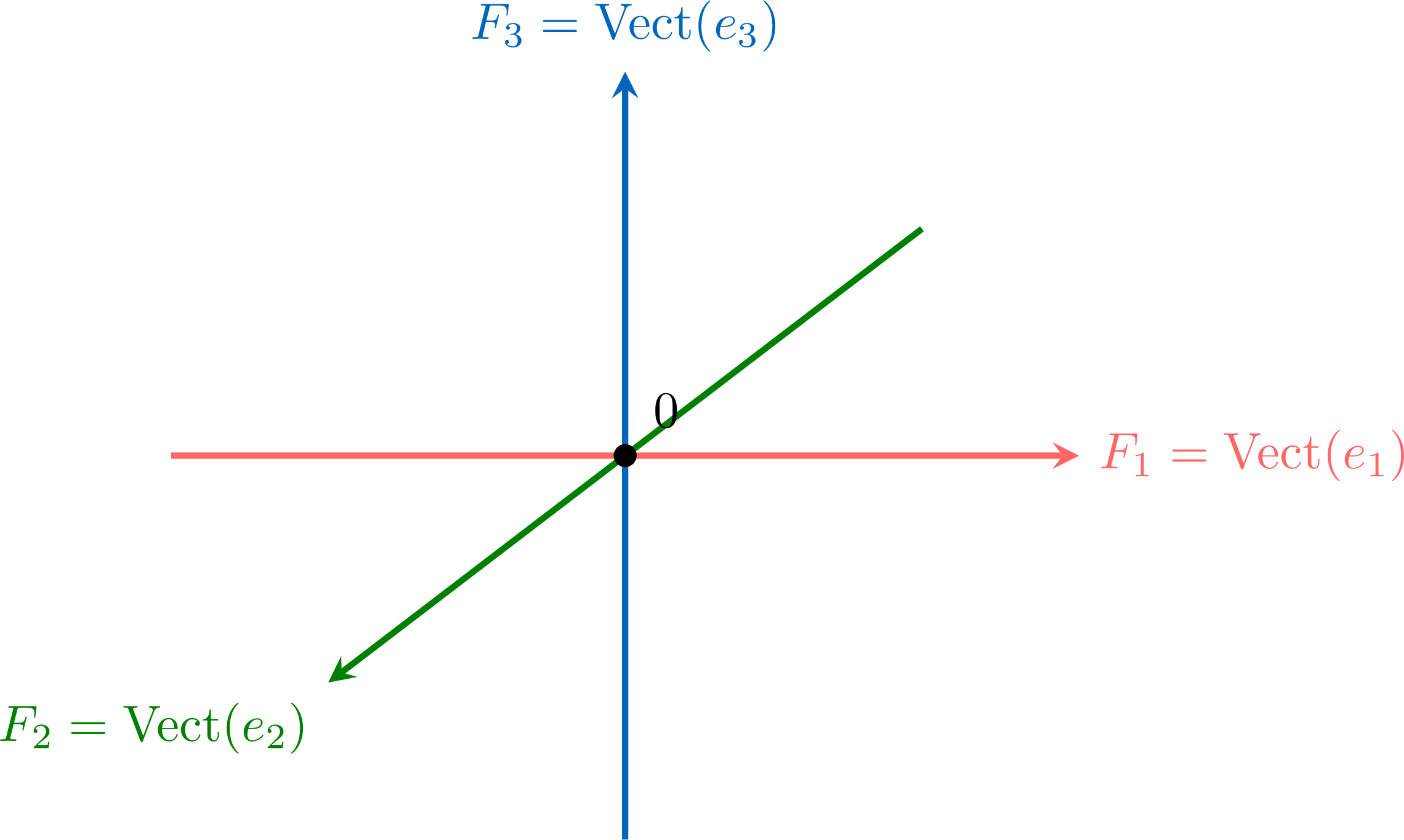

The picture is a flat schematic of the three-dimensional decomposition $\mathbb{R}^3 = F_1 \oplus F_2 \oplus F_3$: the three lines through the origin should be read as three geometrically independent axes (one per dimension), not as coplanar lines. Each vector of $\mathbb{R}^3$ decomposes uniquely as a sum of three components, one in each line. The adapted basis is $(e_1, e_2, e_3)$.

Skills to practice

Constructing an adapted basis
Computing the dimension of a direct sum

II Change of basis

The matrix of an endomorphism depends on the choice of basis. The aim of this section is to express this dependence quantitatively: given two bases $B$ and $B'$ of $E$, what is the link between $\mathrm{Mat}_B(f)$ and $\mathrm{Mat}_{B'}(f)$? The link is provided by the change-of-basis matrix $P_{B, B'}$, and the headline formula is $\mathrm{Mat}_{B'}(f) = P_{B, B'}^{-1}\, \mathrm{Mat}_B(f)\, P_{B, B'}$. This relation between two matrices representing the same endomorphism in two different bases is recorded under the name similarity.

II.1 Recall: matrix of an endomorphism, change-of-basis matrix

We recall, without proof, the constructions of the previous course: the matrix of an endomorphism in a given basis, and the change-of-basis matrix between two bases. The notation $P_{B, B'}$ is locked here for use in the formulas of the next subsection.

Definition — Change-of-basis matrix

This is the same definition as in the previous course, restated here to lock the notation $P_{B, B'}$ for use in the formulas of the next subsection. Let $B = (e_1, \dots, e_n)$ and $B' = (e'_1, \dots, e'_n)$ be two bases of $E$. The change-of-basis matrix from $B$ to $B'$, written $P_{B, B'}$, is the matrix of $\mathcal{M}_n(\mathbb{R})$ whose $j$-th column contains the coordinates of $e'_j$ in the basis $B$: $$ P_{B, B'} \;=\; \mathrm{Mat}_B(e'_1, \dots, e'_n) \;=\; \bigl(\, \mathrm{coord}_B(e'_1) \mid \dots \mid \mathrm{coord}_B(e'_n)\, \bigr). $$

Example

In $\mathbb{R}^2$, take $B = (e_1, e_2)$ the canonical basis, and $B' = (e'_1, e'_2)$ obtained by a rotation of angle $\pi/4$: $$ e'_1 = \tfrac{\sqrt{2}}{2}\, e_1 + \tfrac{\sqrt{2}}{2}\, e_2, \qquad e'_2 = -\tfrac{\sqrt{2}}{2}\, e_1 + \tfrac{\sqrt{2}}{2}\, e_2. $$ Reading off the coordinates as columns: $$ P_{B, B'} \;=\; \begin{pmatrix} \tfrac{\sqrt{2}}{2} & -\tfrac{\sqrt{2}}{2} \\ \tfrac{\sqrt{2}}{2} & \tfrac{\sqrt{2}}{2} \end{pmatrix}. $$

Proposition — Inverse of the change-of-basis matrix

For any two bases $B$ and $B'$ of $E$, the matrix $P_{B, B'}$ is invertible, and $$ \bigl(P_{B, B'}\bigr)^{-1} \;=\; P_{B', B}. $$

Proof

By construction, $P_{B, B'}$ is the matrix of the identity endomorphism $\mathrm{Id}_E$ read from $B'$ to $B$: the $j$-th column of $P_{B, B'}$ is $\mathrm{coord}_B(\mathrm{Id}_E(e'_j)) = \mathrm{coord}_B(e'_j)$. Symmetrically, $P_{B', B}$ reads $\mathrm{Id}_E$ from $B$ to $B'$. Composing the two readings gives the matrix of $\mathrm{Id}_E$ from $B$ to $B$, that is, the identity matrix: $$ \begin{aligned} P_{B, B'} \cdot P_{B', B} &= \mathrm{Mat}_B(\mathrm{Id}_E) && \text{(product equals composition)} \\ &= I_n && \text{(matrix of the identity in any basis)}. \end{aligned} $$ For square matrices, this one-sided identity already implies the other side: any square matrix $M$ satisfying $M\, N = I_n$ also satisfies $N\, M = I_n$ (admitted result of the previous course). Therefore $P_{B, B'}$ is invertible, with inverse $P_{B', B}$.

Example

Continuing the rotation example: a direct $2 \times 2$ inverse computation gives $$ \bigl(P_{B, B'}\bigr)^{-1} \;=\; \begin{pmatrix} \tfrac{\sqrt{2}}{2} & \tfrac{\sqrt{2}}{2} \\ -\tfrac{\sqrt{2}}{2} & \tfrac{\sqrt{2}}{2} \end{pmatrix} \;=\; P_{B', B}, $$ which one can read off directly from the rotation of angle $-\pi/4$ that sends $B'$ back to $B$.

Skills to practice

Computing a change-of-basis matrix

II.2 Change-of-basis formulas

This subsection contains the central formulas of the section. The first is recalled from the previous course; the second is new and will be used throughout the rest of the chapter.

Proposition — Change of coordinates of a vector

Let $B, B'$ be two bases of $E$, and let $x \in E$ with coordinate columns $X_B$ in the basis $B$ and $X_{B'}$ in the basis $B'$. Then $$ X_B = P_{B, B'} \cdot X_{B'}. $$ Recalled from the previous course; no new proof.

Theorem — Change of basis for an endomorphism

Let $f \in \mathcal{L}(E)$ and let $B, B'$ be two bases of $E$. Set $A = \mathrm{Mat}_B(f)$, $A' = \mathrm{Mat}_{B'}(f)$, and $P = P_{B, B'}$. Then $$ A' \;=\; P^{-1}\, A\, P, \qquad \text{i.e.} \qquad \mathrm{Mat}_{B'}(f) \;=\; P_{B, B'}^{-1}\, \mathrm{Mat}_B(f)\, P_{B, B'}. $$

Proof

Take an arbitrary $x \in E$ and write $y = f(x)$. Let $X_B, Y_B$ be the coordinate columns of $x$ and $y$ in the basis $B$, and let $X_{B'}, Y_{B'}$ be the coordinate columns of $x$ and $y$ in the basis $B'$. The matrix of the endomorphism reads the image columnwise: $$ \begin{aligned} Y_B &= A\, X_B && \text{(definition of } A = \mathrm{Mat}_B(f)\text{)}, \\ Y_{B'} &= A'\, X_{B'} && \text{(definition of } A' = \mathrm{Mat}_{B'}(f)\text{)}. \end{aligned} $$ The change-of-coordinates Proposition relates the coordinate columns: $$ \begin{aligned} X_B &= P\, X_{B'}, \\ Y_B &= P\, Y_{B'}. \end{aligned} $$ Substituting in $Y_B = A\, X_B$: $$ \begin{aligned} P\, Y_{B'} &= A\, P\, X_{B'} && \text{(substituting the coordinate-change identities)}, \\ Y_{B'} &= P^{-1}\, A\, P\, X_{B'} && \text{(multiplying on the left by } P^{-1}\text{, which exists by the previous Proposition)}. \end{aligned} $$ This identity holds for every $X_{B'} \in \mathcal{M}_{n, 1}(\mathbb{R})$. Comparing with $Y_{B'} = A'\, X_{B'}$ and specialising $X_{B'}$ to the canonical column vectors $E_1, \dots, E_n$ recovers the columns of $A'$ and of $P^{-1}\, A\, P$ in turn, hence $A' = P^{-1}\, A\, P$.

Example

In $\mathbb{R}^2$, let $f$ be the endomorphism whose matrix in the canonical basis $B = (e_1, e_2)$ is $$ A = \mathrm{Mat}_B(f) = \begin{pmatrix} 2 & 1 \\ 0 & 3 \end{pmatrix}. $$ Consider the basis $B' = (e'_1, e'_2)$ with $e'_1 = e_1$ and $e'_2 = e_1 + e_2$. Compute $\mathrm{Mat}_{B'}(f)$.

Answer

The columns of $P = P_{B, B'}$ are the coordinates of $e'_1, e'_2$ in $B$: $P = \begin{pmatrix} 1 & 1 \\ 0 & 1 \end{pmatrix}$. The inverse is $P^{-1} = \begin{pmatrix} 1 & -1 \\ 0 & 1 \end{pmatrix}$. The change-of-basis formula gives: $$ \begin{aligned} \mathrm{Mat}_{B'}(f) &= P^{-1}\, A\, P && \text{(change of basis for an endomorphism)} \\ &= \begin{pmatrix} 1 & -1 \\ 0 & 1 \end{pmatrix} \begin{pmatrix} 2 & 1 \\ 0 & 3 \end{pmatrix} \begin{pmatrix} 1 & 1 \\ 0 & 1 \end{pmatrix} \\ &= \begin{pmatrix} 1 & -1 \\ 0 & 1 \end{pmatrix} \begin{pmatrix} 2 & 3 \\ 0 & 3 \end{pmatrix} && \text{(right-hand product)} \\ &= \begin{pmatrix} 2 & 0 \\ 0 & 3 \end{pmatrix} && \text{(left-hand product)}. \end{aligned} $$ Cross-check by computing $f(e'_1)$ and $f(e'_2)$ directly: $f(e'_1) = f(e_1) = 2 e_1 = 2 e'_1$ and $f(e'_2) = f(e_1 + e_2) = (2 e_1) + (e_1 + 3 e_2) = 3 e_1 + 3 e_2 = 3 e'_2$. The columns are $\begin{pmatrix} 2 \\ 0 \end{pmatrix}$ and $\begin{pmatrix} 0 \\ 3 \end{pmatrix}$, confirming $\mathrm{Mat}_{B'}(f) = \mathrm{diag}(2, 3)$.

Method — Computing the matrix of $f$ in a new basis

Given $A = \mathrm{Mat}_B(f)$ and a new basis $B'$:

Write $P = P_{B, B'}$ by reading the coordinates of the vectors of $B'$ in $B$ as columns.
Compute $P^{-1}$ (by the methods of the previous course — $2 \times 2$ formula, Gauss elimination, or annihilating polynomial recalled from the previous course).
Compute the product $P^{-1}\, A\, P$.
Verify a column by computing $f$ on a single basis vector $e'_j$ directly.

The verification step is cheap and catches order-of-multiplication errors — in particular the wrong-direction mistake $P\, A\, P^{-1}$.

Skills to practice

Changing the matrix of an endomorphism

II.3 Similar matrices

The change-of-basis formula motivates the notion of similarity: two matrices linked by the formula $B = P^{-1}\, A\, P$ for some invertible $P$ are called similar. This subsection sets up the definition, the equivalence-relation properties, and the central interpretation: similar matrices are exactly two matrices of one and the same endomorphism, expressed in two bases.

Definition — Similar matrices

Two matrices $A, B \in \mathcal{M}_n(\mathbb{R})$ are said to be similar, written $A \sim B$, when there exists $P \in \mathrm{GL}_n(\mathbb{R})$ such that $$ B = P^{-1}\, A\, P. $$

Example

The matrix $I_n$ is similar only to itself: $P^{-1}\, I_n\, P = P^{-1}\, P = I_n$ for every $P \in \mathrm{GL}_n(\mathbb{R})$. More generally, for any $\lambda \in \mathbb{R}$, the scalar matrix $\lambda I_n$ is similar only to itself, since $P^{-1}\, (\lambda I_n)\, P = \lambda\, P^{-1}\, P = \lambda I_n$.

Proposition — Similarity is an equivalence relation

On the set $\mathcal{M}_n(\mathbb{R})$, the relation $\sim$ is an equivalence relation: it is reflexive, symmetric, and transitive.

Proof

Reflexive. For $A \in \mathcal{M}_n(\mathbb{R})$, $A = I_n^{-1}\, A\, I_n$, so $A \sim A$.
Symmetric. Suppose $A \sim B$ via $P$: $B = P^{-1}\, A\, P$. Then $A = P\, B\, P^{-1} = (P^{-1})^{-1}\, B\, (P^{-1})$, which gives $B \sim A$ via $P^{-1}$.
Transitive. Suppose $A \sim B$ via $P$ and $B \sim C$ via $Q$: $B = P^{-1}\, A\, P$ and $C = Q^{-1}\, B\, Q$. Then $$ \begin{aligned} C &= Q^{-1}\, B\, Q && \text{(hypothesis on $B \sim C$)} \\ &= Q^{-1}\, (P^{-1}\, A\, P)\, Q && \text{(substituting $B = P^{-1}\, A\, P$)} \\ &= (P\, Q)^{-1}\, A\, (P\, Q) && \text{(grouping and inverse of a product)}, \end{aligned} $$ and $P\, Q$ is invertible as a product of invertibles. So $A \sim C$ via $P\, Q$.

Theorem — Similarity equals same endomorphism, two bases

Two matrices $A, B \in \mathcal{M}_n(\mathbb{R})$ are similar if and only if there exists an endomorphism $f \in \mathcal{L}(E)$ of some space $E$ of dimension $n$, and two bases $\mathcal{B}_1, \mathcal{B}_2$ of $E$ (possibly equal — in which case $P = I_n$), such that $A = \mathrm{Mat}_{\mathcal{B}_1}(f)$ and $B = \mathrm{Mat}_{\mathcal{B}_2}(f)$.

Proof

Same endomorphism $\Rightarrow$ similar. If $A = \mathrm{Mat}_{\mathcal{B}_1}(f)$ and $B = \mathrm{Mat}_{\mathcal{B}_2}(f)$, set $P = P_{\mathcal{B}_1, \mathcal{B}_2}$. The change-of-basis Theorem of the previous subsection gives $B = P^{-1}\, A\, P$, hence $A \sim B$.
Similar $\Rightarrow$ same endomorphism. Conversely, suppose $B = P^{-1}\, A\, P$ for some $P \in \mathrm{GL}_n(\mathbb{R})$. Take $E = \mathbb{R}^n$ with canonical basis $\mathcal{B}_1$, and let $f$ be the endomorphism of matrix $A$ in $\mathcal{B}_1$. Let $\mathcal{B}_2$ be the basis of $\mathbb{R}^n$ whose vectors are the columns of $P$ (these are linearly independent since $P$ is invertible). Then $P_{\mathcal{B}_1, \mathcal{B}_2} = P$, and the change-of-basis Theorem gives $\mathrm{Mat}_{\mathcal{B}_2}(f) = P^{-1}\, A\, P = B$. So $A$ and $B$ are the two matrices of the same endomorphism $f$ in two bases.

Proposition — Similar matrices have the same rank

If $A, B \in \mathcal{M}_n(\mathbb{R})$ are similar, then $\mathrm{rg}(A) = \mathrm{rg}(B)$.

Proof

By the Theorem above, $A$ and $B$ are the matrices of the same endomorphism $f$ in two bases. Recall from the previous course that the rank of a matrix equals the rank of the linear map it represents: $$ \mathrm{rg}(A) \;=\; \mathrm{rg}(f) \;=\; \mathrm{rg}(B). $$

Example

Show that $A = \begin{pmatrix} 2 & 1 \\ 0 & 3 \end{pmatrix}$ and $B = \begin{pmatrix} 2 & 0 \\ 0 & 3 \end{pmatrix}$ are similar.

Answer

By the worked example of the previous subsection, with $P = \begin{pmatrix} 1 & 1 \\ 0 & 1 \end{pmatrix}$, we computed $P^{-1}\, A\, P = B$. Therefore $A \sim B$ via $P$. (The Theorem above further says that $A$ and $B$ are the two matrices of one and the same endomorphism in two bases of $\mathbb{R}^2$.)

Example — Distinguishing two matrices via rank

Show that $A = \begin{pmatrix} 1 & 0 \\ 0 & 0 \end{pmatrix}$ and $B = \begin{pmatrix} 1 & 0 \\ 0 & 1 \end{pmatrix}$ are not similar.

Answer

Reading off the ranks directly, $\mathrm{rg}(A) = 1$ and $\mathrm{rg}(B) = 2$. By the Proposition above, similar matrices have the same rank; here the ranks differ, so $A$ and $B$ cannot be similar.

Method — Showing two matrices are similar or not similar

To show $A \sim B$: either

exhibit an invertible $P$ such that $B = P^{-1}\, A\, P$ (often by guessing $P$ from a basis change), or
exhibit an endomorphism $f$ and two bases such that $A = \mathrm{Mat}_{\mathcal{B}_1}(f)$ and $B = \mathrm{Mat}_{\mathcal{B}_2}(f)$.

To show $A \not\sim B$: find an invariant of similarity that distinguishes them. At this point in the course, the only invariant available is the rank: if $\mathrm{rg}(A) \ne \mathrm{rg}(B)$, then $A \not\sim B$. The trace, introduced in the next section, will provide a second invariant; the spectrum (eigenvalues) will provide a third, in the next course.

The diagram below summarises the similarity setup.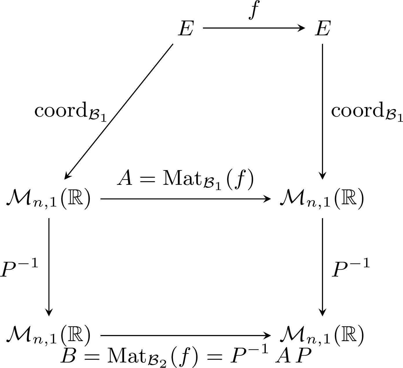

The two matrices $A$ and $B$ read the same endomorphism $f$ in two different bases; the change of coordinates $P$ links the two readings.

Skills to practice

Showing two matrices are similar
Showing two matrices are not similar

III Trace

The trace of a square matrix is the simplest possible invariant: it is just the sum of the diagonal entries. Despite its simplicity, the trace has a remarkable property — it is invariant under similarity, hence under change of basis — which makes it a powerful tool for distinguishing matrices that are not similar, and for defining the trace of an endomorphism (a quantity attached to $f$, not to a specific matrix of $f$).

III.1 Definition and linearity

We first define the trace and observe that it is a linear form on $\mathcal{M}_n(\mathbb{R})$. The proof is a one-line consequence of the linearity of the sum.

Definition — Trace of a square matrix

Let $A = (a_{i, j})_{1 \le i, j \le n} \in \mathcal{M}_n(\mathbb{R})$. The trace of $A$, written $\mathrm{Tr}(A)$, is the sum of its diagonal entries: $$ \mathrm{Tr}(A) \;=\; \sum_{i = 1}^n a_{i, i} \;=\; a_{1, 1} + a_{2, 2} + \dots + a_{n, n}. $$

Example

For $$ A = \begin{pmatrix} 1 & 2 & 3 \\ 4 & 5 & 6 \\ 7 & 8 & 9 \end{pmatrix}, $$ the trace is $\mathrm{Tr}(A) = 1 + 5 + 9 = 15$. Two immediate corner cases: $\mathrm{Tr}(I_n) = n$ (the $n$ diagonal entries are all $1$) and $\mathrm{Tr}(0_n) = 0$ (every entry is zero).

Example

For a diagonal matrix $D = \mathrm{diag}(d_1, \dots, d_n)$, the trace is the sum of the diagonal entries: $$ \mathrm{Tr}(D) \;=\; d_1 + d_2 + \dots + d_n. $$ The same formula holds for a triangular matrix (upper or lower): the off-diagonal entries do not contribute.

Proposition — Linearity of the trace

The map $\mathrm{Tr}: \mathcal{M}_n(\mathbb{R}) \to \mathbb{R}$ is linear. Concretely, for all $A, B \in \mathcal{M}_n(\mathbb{R})$ and $\lambda, \mu \in \mathbb{R}$: $$ \mathrm{Tr}(\lambda A + \mu B) \;=\; \lambda\, \mathrm{Tr}(A) + \mu\, \mathrm{Tr}(B). $$

Proof

Write $A = (a_{i, j})$ and $B = (b_{i, j})$. The $(i, i)$ entry of $\lambda A + \mu B$ is $\lambda a_{i, i} + \mu b_{i, i}$, so $$ \begin{aligned} \mathrm{Tr}(\lambda A + \mu B) &= \sum_{i = 1}^n (\lambda a_{i, i} + \mu b_{i, i}) && \text{(definition of the trace)} \\ &= \lambda \sum_{i = 1}^n a_{i, i} + \mu \sum_{i = 1}^n b_{i, i} && \text{(linearity of the sum)} \\ &= \lambda\, \mathrm{Tr}(A) + \mu\, \mathrm{Tr}(B). \end{aligned} $$

Skills to practice

Computing a trace

III.2 The fundamental identity $\mathrm{Tr}(AB)\equal\mathrm{Tr}(BA)$ and invariance by change of basis

The headline identity of this section is $\mathrm{Tr}(AB) = \mathrm{Tr}(BA)$: the trace is invariant under swapping the two factors of a product. (Beware: this does not extend to arbitrary reorderings of three or more factors — for $A, B, C$, the trace is invariant under cyclic permutations, $\mathrm{Tr}(ABC) = \mathrm{Tr}(BCA) = \mathrm{Tr}(CAB)$, but not under $\mathrm{Tr}(ABC) = \mathrm{Tr}(ACB)$ in general.) Two consequences of the two-factor identity are immediate. First, the trace is invariant under the change of basis $A \mapsto P^{-1}\, A\, P$ — equivalently, two similar matrices have the same trace. Second, the trace of an endomorphism is well defined: it does not depend on the choice of basis used to read its matrix.

Proposition — $\mathrm{Tr}(AB)\equal\mathrm{Tr}(BA)$

For all $A, B \in \mathcal{M}_n(\mathbb{R})$, $$ \mathrm{Tr}(A\, B) \;=\; \mathrm{Tr}(B\, A). $$

Proof

Write $A = (a_{i, j})$ and $B = (b_{i, j})$. The $(i, i)$ entry of the product $A\, B$ is $\sum_{k = 1}^n a_{i, k}\, b_{k, i}$, so $$ \begin{aligned} \mathrm{Tr}(A\, B) &= \sum_{i = 1}^n \sum_{k = 1}^n a_{i, k}\, b_{k, i} && \text{(definition of trace and matrix product)} \\ &= \sum_{k = 1}^n \sum_{i = 1}^n b_{k, i}\, a_{i, k} && \text{(swapping the order of the finite double sum)} \\ &= \sum_{k = 1}^n (B\, A)_{k, k} && \text{(the inner sum is the $(k, k)$ entry of $B\, A$)} \\ &= \mathrm{Tr}(B\, A). \end{aligned} $$

Theorem — Invariance of the trace by change of basis

For all $A \in \mathcal{M}_n(\mathbb{R})$ and $P \in \mathrm{GL}_n(\mathbb{R})$, $$ \mathrm{Tr}(P^{-1}\, A\, P) \;=\; \mathrm{Tr}(A). $$

Proof

We apply the Proposition $\mathrm{Tr}(X\, Y) = \mathrm{Tr}(Y\, X)$ with the regrouping $X = P^{-1}\, A$ and $Y = P$: $$ \begin{aligned} \mathrm{Tr}(P^{-1}\, A\, P) &= \mathrm{Tr}\bigl( (P^{-1}\, A)\, P\bigr) && \text{(regrouping the factors)} \\ &= \mathrm{Tr}\bigl( P\, (P^{-1}\, A)\bigr) && \text{(by the Proposition $\mathrm{Tr}(XY) = \mathrm{Tr}(YX)$)} \\ &= \mathrm{Tr}\bigl( (P\, P^{-1})\, A\bigr) && \text{(associativity)} \\ &= \mathrm{Tr}(I_n\, A) && \text{(since $P\, P^{-1} = I_n$)} \\ &= \mathrm{Tr}(A) && \text{($I_n\, A = A$)}. \end{aligned} $$

Proposition — Similar matrices have the same trace

If $A, B \in \mathcal{M}_n(\mathbb{R})$ are similar, then $\mathrm{Tr}(A) = \mathrm{Tr}(B)$.

Proof

By the definition of similarity, $B = P^{-1}\, A\, P$ for some $P \in \mathrm{GL}_n(\mathbb{R})$. The previous Theorem gives $\mathrm{Tr}(B) = \mathrm{Tr}(P^{-1}\, A\, P) = \mathrm{Tr}(A)$.

Same trace does not imply similar

The converse of the Proposition above is false. For instance, $$ I_2 = \begin{pmatrix} 1 & 0 \\ 0 & 1 \end{pmatrix} \qquad \text{and} \qquad C = \begin{pmatrix} 2 & 0 \\ 0 & 0 \end{pmatrix} $$ both have trace equal to $2$, yet they are not similar: $I_2$ has rank $2$ whereas $C$ has rank $1$, and the rank is an invariant of similarity. The trace is a necessary, not sufficient, condition for similarity.

Definition — Trace of an endomorphism

Let $f \in \mathcal{L}(E)$. The trace of $f$, written $\mathrm{Tr}(f)$, is the trace of the matrix of $f$ in any basis of $E$: $$ \mathrm{Tr}(f) \;=\; \mathrm{Tr}\bigl( \mathrm{Mat}_B(f)\bigr) \qquad \text{for any basis } B \text{ of } E. $$ This definition does not depend on the chosen basis $B$, since two matrices of $f$ in different bases are similar (by the Theorem of the previous section), hence have the same trace.

Example

$\mathrm{Tr}(\mathrm{Id}_E) = \mathrm{Tr}(I_n) = n = \dim E$ (the identity has matrix $I_n$ in every basis).

Example — Trace of a specific projector

In $E = \mathbb{R}^3$, set $F = \mathrm{Vect}(e_1, e_2)$ and $G = \mathrm{Vect}(e_3)$, and let $p$ be the projector onto $F$ parallel to $G$ (the map that sends $(x, y, z)$ to $(x, y, 0)$). In the adapted basis $\mathcal{B} = (e_1, e_2, e_3)$, the matrix reads $$ \mathrm{Mat}_{\mathcal{B}}(p) \;=\; \mathrm{diag}(1, 1, 0), $$ so $\mathrm{Tr}(p) = 1 + 1 + 0 = 2$. By the invariance Theorem, this trace value does not depend on the basis we used; it is an intrinsic quantity attached to $p$.

Method — Computing the trace via an adapted basis

When an endomorphism $f$ has a known block structure in some adapted basis $\mathcal{B}$ (for instance, $\mathcal{B}$ adapted to a direct-sum decomposition that $f$ respects — a projector, a symmetry, or any operator built from the decomposition), the strategy is:

Choose the adapted basis $\mathcal{B}$.
Write the matrix $\mathrm{Mat}_{\mathcal{B}}(f)$ block by block.
Read $\mathrm{Tr}(f)$ as the sum of the diagonal entries.

This avoids the need to write $f$ in an arbitrary basis and then change back, often turning the computation into a one-line read-off.

Method — Using the trace as a non-similarity invariant

To show $A \not\sim B$:

Compute $\mathrm{Tr}(A)$ and $\mathrm{Tr}(B)$.
If $\mathrm{Tr}(A) \ne \mathrm{Tr}(B)$, conclude $A \not\sim B$ (since similar matrices share their trace).

Combined with the rank invariant of the previous section, this gives the two practical invariants for similarity questions at this stage of the course. The two are independent: $\begin{pmatrix} 1 & 0 \\ 0 & 0 \end{pmatrix}$ and $\begin{pmatrix} 0 & 1 \\ 0 & 0 \end{pmatrix}$ have the same rank ($1$) but different traces; conversely, the example of the previous Remark gives two matrices with the same trace but different ranks. Beware: matching trace and rank does not imply similarity, even taken together. The next course introduces a finer family of invariants (eigenvalues with their multiplicities), which refines the rank/trace test.

Going further

The three pillars of this course — direct sums, change of basis, and trace — feed directly into the next course, which studies the reduction of endomorphisms. The central question there is: given an endomorphism $f$, can one find a basis $B'$ in which $\mathrm{Mat}_{B'}(f)$ is as simple as possible — ideally, diagonal? The answer leads to the notions of eigenvalue, eigenvector and diagonalisability, and the trace becomes the simplest tool to spot the sum of eigenvalues. The direct-sum machinery is the framework in which the diagonal decomposition is naturally expressed, and the change-of-basis formula is the operative tool that turns the abstract decomposition into a concrete matrix computation.

Skills to practice

Using the trace as an invariant

IV Going further

Skills to practice

Combining direct sums and trace