International Baccalaureate · DP 2: Applications and Interpretation HL
Revision: Statistics and Probability
I
Toolbox: Expected Frequencies and Degrees of Freedom
Recappreviously studied — click to reread
Definition — Observed and Expected Frequencies
- Observed Frequencies (\(f_o\)): The actual counts collected and recorded in a contingency table.
- Expected Frequencies (\(f_e\)): The theoretical counts calculated assuming the variables are independent.
Definition — Chi-squared Statistic
The test statistic \(\chi^2_{calc}\) measures the total deviation between observed and expected values:$$ \chi^2_{calc} = \sum \frac{(f_o - f_e)^2}{f_e} $$ The degrees of freedom (\(df\)) for a table with \(r\) rows and \(c\) columns is:$$ \mathrm{d}f = (r - 1)(c - 1) $$ Example
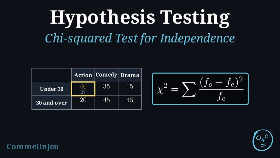
A survey asked 200 people about their preferred type of movie and their age group. The results are shown below: | Action | Comedy | Drama | |
| Under 30 | 40 | 35 | 15 |
| 30 and over | 20 | 45 | 45 |
- Step 1: Hypotheses
\(H_0\): Age group and movie preference are independent.
\(H_1\): Age group and movie preference are not independent (they are associated). - Step 2: Calculator
Enter the \(2 \times 3\) matrix into the calculator and run the \(\chi^2\)-Test.- \(\chi^2_{calc} \approx 21.1\)
- \(\mathrm{d}f = (2-1)(3-1) = 2\)
- \(p\text{-value} \approx 0.000026\) (about \(2.6 \times 10^{-5}\))
- Step 3: Conclusion
\(0.000026 < 0.05\). Since \(p < \alpha\), we reject \(H_0\).
There is strong evidence to suggest that movie preference depends on age group.
Skills to practice
- Finding Expected Frequencies and Degrees of Freedom
II
Toolbox: Normal Probabilities and the Inverse Normal
Recappreviously studied — click to reread
Method — Calculating a Normal Probability with Technology
For \(X \sim \mathcal{N}(\mu, \sigma^2)\), the probability of an interval is an area under the normal curve, an integral of the density whose antiderivative cannot be written with the usual functions (polynomials, exponentials, logarithms): the normal cumulative distribution function of a graphing calculator computes it. Its name depends on the model: Normal C.D, normalcdf, normCdf. - State the model: \(X \sim \mathcal{N}(\mu, \sigma^2)\), with its mean \(\mu\) and its standard deviation \(\sigma\) — not the variance \(\sigma^2\): for \(X \sim \mathcal{N}(50, 16)\), \(\sigma = 4\).
- Sketch and shade first: draw a bell curve centred at \(\mu\), mark the bound or bounds, and shade the region of the event. The sketch predicts the size of the answer: a region that contains the mean and most of the curve has a probability close to \(1\), a region that lies on one side of \(\mu\) a probability less than \(0.5\), and a region far in one tail a probability close to \(0\).
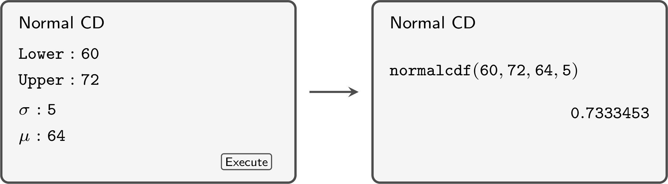
- Enter the bounds of the region, as in the table below, then \(\mu\) and \(\sigma\), each in the field that carries its name: the order of the fields depends on the model, and the command
normalcdftakes the lower bound, the upper bound, \(\mu\), then \(\sigma\). A region with no left end takes as its lower bound a negative number so large that it lies very many standard deviations below the mean, such as \(-10^{99}\), and a region with no right end a positive number as large, such as \(10^{99}\), as its upper bound. - Compare the screen with the sketch, and report the probability to \(3\) significant figures, unless the question asks otherwise.
| Event | Lower bound | Upper bound |
| \(a < X < b\) | \(a\) | \(b\) |
| \(X < b\) | \(-10^{99}\) | \(b\) |
| \(X > a\) | \(a\) | \(10^{99}\) |
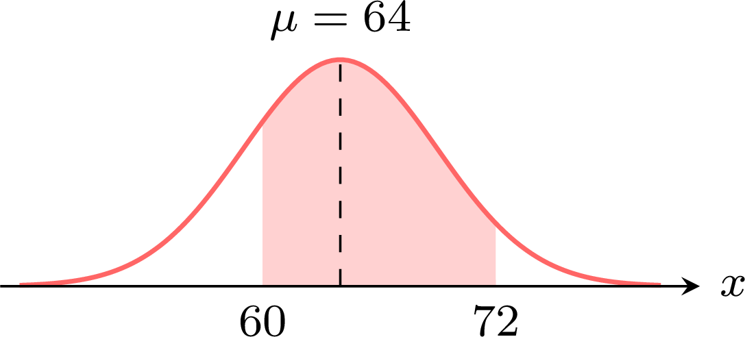
The sketch and the mock-up show the computation of \(P(60 < X < 72)\) for \(X \sim \mathcal{N}(64, 5^2)\): the region contains the mean and most of the curve, and the screen gives \(P(60 < X < 72) \approx 0.733\).
Method — Finding a Value with the Inverse Normal Function
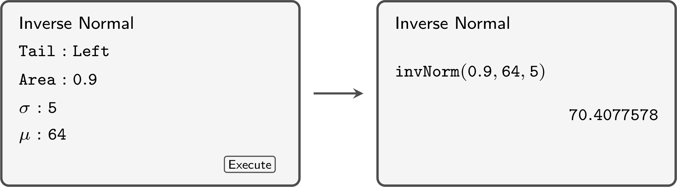
The reverse question gives a probability and asks for a value of \(X\). The inverse normal function of the calculator (Inverse Normal, invNorm) returns the value \(k\) such that \(P(X < k) = p\), for \(0 < p < 1\), from the area \(p\) to the left of \(k\), \(\sigma\) and \(\mu\). - State the model \(X \sim \mathcal{N}(\mu, \sigma^2)\) and name the unknown value \(k\).
- Sketch and shade: place \(k\) on the side of \(\mu\) that the probability indicates — a left area less than \(0.5\) puts \(k\) below the mean — and shade the given area.
- Turn the condition into a left area. The condition \(P(X < k) = p\) is entered as it is; \(P(X > k) = q\) becomes \(P(X < k) = 1 - q\). An interval centred on \(\mu\) that contains the proportion \(p\) of the values leaves \(\frac{1 - p}{2}\) in each tail: its ends are the values with left areas \(\frac{1 - p}{2}\) and \(\frac{1 + p}{2}\).
- Enter the area, \(\mu\) and \(\sigma\), each in its field (the command
invNormtakes the area, \(\mu\), then \(\sigma\); the tail is set to the left, on the models that ask for one), then check the position of \(k\) against the sketch and report it to \(3\) significant figures, or to the precision of the data.
Example
The scores \(X\) on an entrance test are normally distributed with mean \(500\) and standard deviation \(80\). - A scholarship is offered to the top \(12\pourcent\) of the candidates. Find the minimum score for a scholarship.
- The lowest \(5\pourcent\) of the candidates are offered extra support. Find the score below which a candidate is offered support.
The model is \(X \sim \mathcal{N}(500, 80^2)\). 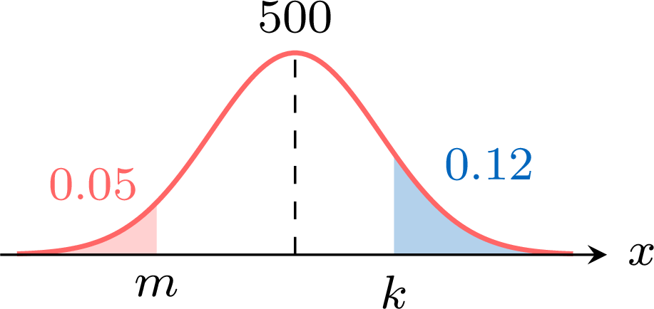
- Let \(k\) be the minimum score: \(P(X > k) = 0.12\). The right tail is small, so \(k\) lies above the mean. As a left area, $$\begin{aligned}[t] P(X < k) &= 1 - P(X > k) && \text{(complementary event)}\\ &= 1 - 0.12\\ &= 0.88. \end{aligned}$$ The inverse normal function with area \(0.88\), \(\sigma = 80\) and \(\mu = 500\) gives \(593.9989\ldots\): the minimum score for a scholarship is about \(594\).
- Let \(m\) be the score: \(P(X < m) = 0.05\), a left tail, so \(m\) lies below the mean. The inverse normal function with area \(0.05\), \(\sigma = 80\) and \(\mu = 500\) gives \(368.4117\ldots\): a candidate who scores below about \(368\) is offered support.
Skills to practice
- Calculating Normal Probabilities and Values
III
Exam-Style Questions
Skills to practice
- Working with Technology: Statistics and Probability
- Working with Technology: Further Statistics and Probability
Jump to section