International Baccalaureate · DP 2: Applications and Interpretation HL

Markov Chains

⌚ ~98 min ▢ 10 blocks ✓ 53 exercises ➣ Prerequisites : Matrices, Eigenvalues and Eigenvectors, Conditional Probability

I Markov Chains

I.1 Markov Chain

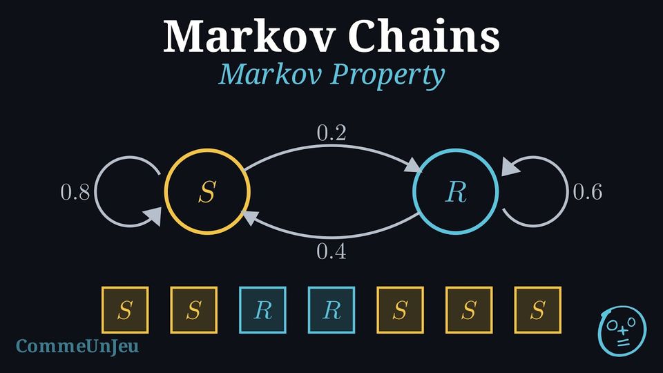
In many real-world models, we assume deterministic outcomes based on formulas. However, many systems involve random variation.
A stochastic model uses probability to predict outcomes where randomness is present.
A Markov chain is a specific type of stochastic model that describes a sequence of events where the probability of each event depends only on the state attained in the previous event. This is known as the memoryless or Markov property.

Report an error

Definition

A Markov chain is a sequence of random variables describing a system that transitions between different states. The key property is that the probability of moving to the next state depends only on the current state and not on the sequence of events that preceded it.

Definition — Transition Diagram

A transition diagram illustrates the states of a system and the probabilities of moving from one state to another.

States are represented by circles (nodes).
Arrows show movement (transitions) between states.
Each arrow is labelled with a transition probability.
The sum of probabilities on outgoing arrows from any state must equal 1.

Example

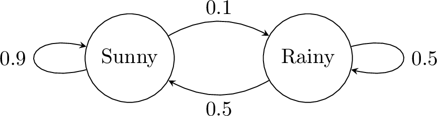
If it is Sunny today, there is a $0.9$ probability it will be Sunny tomorrow (loop) and $0.1$ probability it will be Rainy.
If it is Rainy today, there is a $0.5$ probability it will be Sunny tomorrow and $0.5$ probability it will be Rainy.

Skills to practice

Reading Transition Diagrams

I.2 Matrix Representation

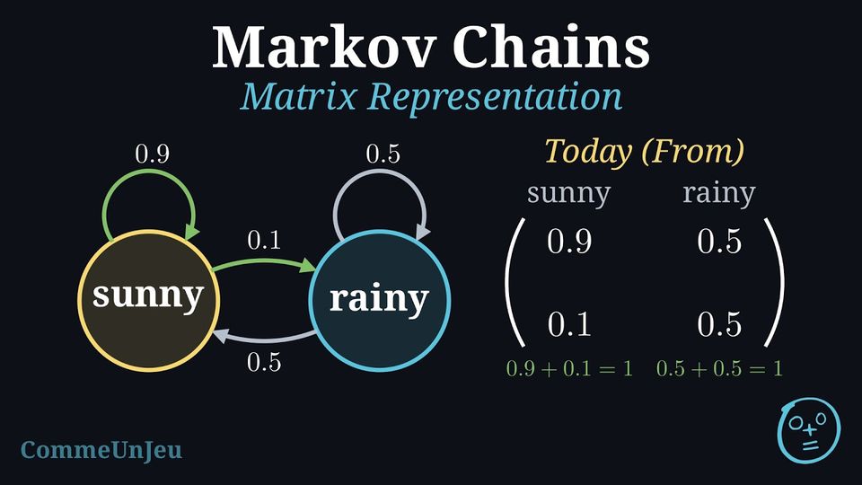
A powerful method for studying Markov chains is to represent the probabilities and states using matrices. This allows for rapid calculation of future states using matrix multiplication.

Report an error

Definition — State Vector

The state vector $\mathbf{s}_n$ is a column vector that shows the probability distribution of the system at time step $n$.

It represents the probability or proportion of being in each state.
The sum of the elements in a state vector is always 1.
The initial state is denoted by $\mathbf{s}_0$.

Example

If today is certainly Sunny, the initial state matrix is $\mathbf{s}_0 = \begin{pmatrix} 1 \\ 0 \end{pmatrix}$.

Definition — Transition Matrix

The transition matrix $\mathbf{T}$ organizes the transition probabilities into a square matrix.
In a transition matrix $\mathbf{T} = (t_{ij})$:

The columns represent the current state (From).
The rows represent the next state (To).
The entry $t_{ij}$ represents the probability of moving to state $i$ from state $j$.
The sum of each column must be 1.

Example

For the weather example: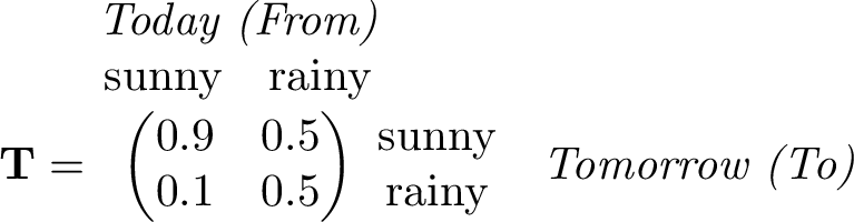

The States Are Events

Let $X_n$ be the state of the system after $n$ steps, the states being numbered $1, 2, \dots, k$ ($X_0$ is the initial state): $X_n$ is a random variable. For each state $j$, $(X_n = j)$ is an event, the set of the outcomes in which the system is in state $j$ after $n$ steps. For a fixed $n$, the $k$ events $(X_n = 1), \dots, (X_n = k)$ form a partition of the sample space $U$, since after $n$ steps the system is in exactly one state. The vectors and the matrix of the chain are read with these events:

the state vector $\mathbf{s}_n$ is the probability distribution of $X_n$: its entry in row $i$ is $P(X_n = i)$;
the entry $t_{ij}$ of the transition matrix is a conditional probability, $t_{ij} = \PCond{X_{n+1} = i}{X_n = j}$: the probability that the system is in state $i$ at the next step, given that it is in state $j$ now (defined when $P(X_n = j) > 0$).

The chain is homogeneous when a single transition matrix $\mathbf{T}$, given by the model, serves for every step: its entries are non-negative, each of its columns sums to $1$, and $t_{ij} = \PCond{X_{n+1} = i}{X_n = j}$ at every step $n$ such that $P(X_n = j) > 0$. When $P(X_n = j) > 0$, the column sum is no extra assumption: given $(X_n = j)$, the events $(X_{n+1} = 1), \dots, (X_{n+1} = k)$ again form a partition, so their conditional probabilities add up to $1$.

Report an error

Skills to practice

Defining and Validating State Vectors
Building and Interpreting Transition Matrices

II State Vectors and Future Probabilities

II.1 Calculating Future States

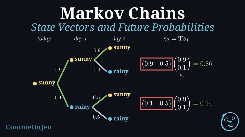
Proposition — The Next State Vector

For a homogeneous Markov chain with states $1, \dots, k$, transition matrix $\mathbf{T}$ and state vectors $\mathbf{s}_0, \mathbf{s}_1, \mathbf{s}_2, \dots$: $$\textcolor{colorprop}{\mathbf{s}_{n+1} = \mathbf{T}\mathbf{s}_n} \ \text{ for every } n \geq 0, \qquad \text{hence} \qquad \textcolor{colorprop}{\mathbf{s}_n = \mathbf{T}^n\mathbf{s}_0} \ \text{ for every } n \geq 1.$$

Proof

The step from $n$ to $n + 1$. Let $n \geq 0$ and let $i$ be a state. The events $(X_n = 1), \dots, (X_n = k)$ form a partition of the sample space, so, by the Proposition “Partition Induced on an Event”, the event $(X_{n+1} = i)$ is cut into the pieces $(X_{n+1} = i) \cap (X_n = j)$, for $j = 1, \dots, k$, which are pairwise mutually exclusive. For each state $j$, two cases arise:

if $P(X_n = j) > 0$, the Joint Probability Formula gives $P\big((X_{n+1} = i) \cap (X_n = j)\big) = P(X_n = j) \times \PCond{X_{n+1} = i}{X_n = j} = t_{ij}\,P(X_n = j)$;
if $P(X_n = j) = 0$, the conditional probability given $(X_n = j)$ is not defined; but the piece is contained in $(X_n = j)$, so, by Axiom 1 and the Proposition “Monotonicity”, its probability lies between $0$ and $P(X_n = j) = 0$: it is $0$, which is again $t_{ij}\,P(X_n = j) = t_{ij} \times 0$.

So, for every state $i$, $$\begin{aligned}[t] P(X_{n+1} = i) &= \sum_{j=1}^{k} P\big((X_{n+1} = i) \cap (X_n = j)\big) && \text{(additivity over the pieces)}\\ &= \sum_{j=1}^{k} t_{ij}\,P(X_n = j) && \text{(the two cases above)}\\ &= t_{i1}P(X_n = 1) + t_{i2}P(X_n = 2) + \dots + t_{ik}P(X_n = k). \end{aligned}$$ This is the law of total probability, written so that it also covers the states of probability $0$. The left-hand side is the entry in row $i$ of $\mathbf{s}_{n+1}$; the right-hand side is row $i$ of $\mathbf{T}$ multiplied by the column $\mathbf{s}_n$, that is, the entry in row $i$ of $\mathbf{T}\mathbf{s}_n$. The two columns have the same entries: $\mathbf{s}_{n+1} = \mathbf{T}\mathbf{s}_n$. The formula $\mathbf{s}_n = \mathbf{T}^n\mathbf{s}_0$, by induction. Let $\mathcal{P}(n)$ be the proposition “$\mathbf{s}_n = \mathbf{T}^n\mathbf{s}_0$”.

Base case: the first part with $n = 0$ gives $\mathbf{s}_1 = \mathbf{T}\mathbf{s}_0 = \mathbf{T}^1\mathbf{s}_0$, so $\mathcal{P}(1)$ is true.
Inductive step: assume $\mathcal{P}(m)$ for some $m \geq 1$ (inductive hypothesis). Then $$\begin{aligned}[t] \mathbf{s}_{m+1} &= \mathbf{T}\mathbf{s}_m && \text{(first part)}\\ &= \mathbf{T}(\mathbf{T}^m\mathbf{s}_0) && \text{(by the inductive hypothesis)}\\ &= \mathbf{T}^{m+1}\mathbf{s}_0 && \text{(associativity of the matrix product)} \end{aligned}$$ so $\mathcal{P}(m+1)$ is true.

Since $\mathcal{P}(1)$ is true and $\mathcal{P}(m) \Rightarrow \mathcal{P}(m+1)$, by the principle of mathematical induction, $\mathbf{s}_n = \mathbf{T}^n\mathbf{s}_0$ for all $n \geq 1$.

Method — Calculating Future States

To predict the probability distribution of the system after $n$ steps, we multiply the transition matrix by the state vector repeatedly.
The general formula is:$$ \mathbf{s}_n = \mathbf{T}^n \mathbf{s}_0 $$ where $\mathbf{T}$ is the transition matrix and $\mathbf{s}_0$ is the initial state vector.

$\mathbf{s}_1 = \mathbf{T} \mathbf{s}_0$ (State after 1 step)
$\mathbf{s}_2 = \mathbf{T} \mathbf{s}_1 = \mathbf{T}(\mathbf{T}\mathbf{s}_0) = \mathbf{T}^2 \mathbf{s}_0$ (State after 2 steps)

Example

Using the weather matrix $\mathbf{T} = \begin{pmatrix} 0.9 & 0.5 \\ 0.1 & 0.5 \end{pmatrix}$ and assuming it is Sunny today ($\mathbf{s}_0 = \begin{pmatrix} 1 \\ 0 \end{pmatrix}$), calculate the probabilities for the weather in 2 days.

Answer

$$ \begin{aligned} \mathbf{s}_2 &= \mathbf{T}^2 \mathbf{s}_0\\ &= \begin{pmatrix} 0.9 & 0.5 \\ 0.1 & 0.5 \end{pmatrix}^2 \begin{pmatrix} 1 \\ 0 \end{pmatrix} \\ &= \begin{pmatrix} 0.9 & 0.5 \\ 0.1 & 0.5 \end{pmatrix} \begin{pmatrix} 0.9 & 0.5 \\ 0.1 & 0.5 \end{pmatrix} \begin{pmatrix} 1 \\ 0 \end{pmatrix}\\ &= \begin{pmatrix} (0.9)(0.9)+(0.5)(0.1) & (0.9)(0.5)+(0.5)(0.5) \\ (0.1)(0.9)+(0.5)(0.1) & (0.1)(0.5)+(0.5)(0.5) \end{pmatrix} \begin{pmatrix} 1 \\ 0 \end{pmatrix}\\ &= \begin{pmatrix} 0.86 & 0.70 \\ 0.14 & 0.30 \end{pmatrix} \begin{pmatrix} 1 \\ 0 \end{pmatrix}\\ &= \begin{pmatrix} 0.86 \\ 0.14 \end{pmatrix}. \end{aligned} $$ Interpretation: There is an $86\pourcent$ chance it will be Sunny and a $14\pourcent$ chance it will be Rainy in 2 days.

Example

Each month, the $8000$ commuters of a town travel by bus, by car or by bike. Of the bus users, $70\pourcent$ keep the bus the next month, $20\pourcent$ change to the car and $10\pourcent$ to the bike. Of the car users, $10\pourcent$ change to the bus, $80\pourcent$ keep the car and $10\pourcent$ change to the bike. Of the bike users, $20\pourcent$ change to the bus, $10\pourcent$ to the car and $70\pourcent$ keep the bike. This month, $3000$ commuters take the bus, $4000$ the car and $1000$ the bike.

Write the transition matrix $\mathbf{T}$, with the states in the order bus, car, bike.
Find, by hand, the expected number of commuters in each group next month.
Using technology, find $\mathbf{T}^2$ and interpret the entry in row $3$ and column $1$.
Using technology, find the expected number of commuters in each group in $6$ months, to the nearest whole number.

Answer

Column $j$ lists the probabilities of moving from state $j$ to each state: $$\mathbf{T} = \begin{pmatrix} 0.7 & 0.1 & 0.2 \\ 0.2 & 0.8 & 0.1 \\ 0.1 & 0.1 & 0.7 \end{pmatrix},$$ each column summing to $1$.
With the numbers of commuters instead of probabilities, the column $\mathbf{s}_0$ is a vector of counts, whose entries add up to $8000$ instead of $1$: $\mathbf{s}_0 = \begin{pmatrix} 3000 \\ 4000 \\ 1000 \end{pmatrix}$. Each entry of $\mathbf{T}\mathbf{s}_0$ adds, over the three groups, the number of commuters in the group times the probability of moving to the state of the row, so it is the expected number in that state: $$\mathbf{s}_1 = \mathbf{T}\mathbf{s}_0 = \begin{pmatrix} 0.7 \times 3000 + 0.1 \times 4000 + 0.2 \times 1000 \\ 0.2 \times 3000 + 0.8 \times 4000 + 0.1 \times 1000 \\ 0.1 \times 3000 + 0.1 \times 4000 + 0.7 \times 1000 \end{pmatrix} = \begin{pmatrix} 2700 \\ 3900 \\ 1400 \end{pmatrix}.$$ About $2700$ commuters are expected on the bus, $3900$ in a car and $1400$ on a bike; the total is still $8000$.
The calculator gives $$\mathbf{T}^2 = \begin{pmatrix} 0.53 & 0.17 & 0.29 \\ 0.31 & 0.67 & 0.19 \\ 0.16 & 0.16 & 0.52 \end{pmatrix}.$$ Since $\mathbf{s}_2 = \mathbf{T}^2\mathbf{s}_0$, $\mathbf{T}^2$ is the transition matrix over two months: the entry $0.16$ in row $3$ and column $1$ is the probability that a commuter who takes the bus this month rides a bike two months later.
By the Method “Calculating Future States”, $\mathbf{s}_6 = \mathbf{T}^6\mathbf{s}_0$, and the calculator gives $$\mathbf{s}_6 = \begin{pmatrix} 2476.672 \\ 3569.984 \\ 1953.344 \end{pmatrix}.$$ In $6$ months, about $2477$ commuters are expected on the bus, $3570$ in a car and $1953$ on a bike.

Skills to practice

Predicting States with Technology
Calculating and Predicting States after One or Two Steps

III Steady State

III.1 Steady State

Definition — Steady State Vector

For many regular Markov chains (a chain is regular if some power of $\mathbf{T}$ has all-positive entries), as the number of steps increases ($n \to \infty$), the state vector $\mathbf{s}_n$ converges to a constant vector $\mathbf{s}$, regardless of the initial state $\mathbf{s}_0$.
This vector $\mathbf{s}$ is called the steady state vector (or stationary distribution).
It satisfies the equilibrium equation:$$ \mathbf{T} \mathbf{s} = \mathbf{s} $$ Algebraically, $\mathbf{s}$ is an eigenvector of $\mathbf{T}$ corresponding to the eigenvalue $\lambda = 1$. The sum of the elements of $\mathbf{s}$ must be 1.

Method — Finding the Steady State

To find the steady state vector $\mathbf{s} = \begin{pmatrix} x \\ y \end{pmatrix}$:

Set up the matrix equation $\mathbf{T}\mathbf{s} = \mathbf{s}$.
Convert this into a system of linear equations.
Use the additional constraint $x + y = 1$ (for a 2-state system) to solve for $x$ and $y$.

Example

A city operates a bike-sharing system with two main zones: the City Centre (C) and the Train Station (S).
Bikes are rented and returned daily. The transition matrix $\mathbf{T}$ represents the probability of a bike moving between zones or staying in the same zone by the end of the day:$$ \mathbf{T} = \begin{pmatrix} 0.8 & 0.3 \\ 0.2 & 0.7 \end{pmatrix} $$

Find the steady state vector $\mathbf{s} = \begin{pmatrix} x \\ y \end{pmatrix}$ algebraically.
If the city owns $1000$ bikes in total, determine how they should be distributed between the City Centre and the Train Station in the long run to meet demand.

Answer

Find an eigenvector for $\lambda = 1$:
$$\begin{aligned} \mathbf{T}\mathbf{s} &= \mathbf{s}\\ \begin{pmatrix} 0.8 & 0.3 \\ 0.2 & 0.7 \end{pmatrix}\begin{pmatrix} x \\ y \end{pmatrix} &= \begin{pmatrix} x \\ y \end{pmatrix}\\ \begin{pmatrix} 0.8x+0.3y \\ 0.2x+0.7y \end{pmatrix} &= \begin{pmatrix} x \\ y \end{pmatrix}\\ \end{aligned}$$ This gives $0.8x+0.3y = x$ and $0.2x+0.7y=y$.
Simplifying, we get $-0.2x+0.3y = 0$ and $0.2x-0.3y=0$.
Thus $0.2x = 0.3y$, which implies $2x = 3y$.
Letting $y = 2t$, we have $x = 3t$, so: $$ \mathbf{s} = \begin{pmatrix} 3t \\ 2t \end{pmatrix}$$ Since $\mathbf{s}$ is a state vector, the sum of its components must be 1: $$ 3t + 2t = 1 \implies 5t = 1 \implies t = \frac{1}{5} $$ $$ \mathbf{s} = \begin{pmatrix} 3 \cdot \frac{1}{5} \\ 2 \cdot \frac{1}{5} \end{pmatrix} = \begin{pmatrix} 0.6 \\ 0.4 \end{pmatrix} $$
In the long run, $60\pourcent$ of the bikes will be at the City Centre and $40\pourcent$ at the Train Station.
- City Centre: $1000 \times 0.6 = 600$ bikes.
- Train Station: $1000 \times 0.4 = 400$ bikes.

Method — Long-Term Probabilities by Repeated Multiplication

For a regular chain, $\mathbf{s}_n = \mathbf{T}^n\mathbf{s}_0$ approaches the steady state vector $\mathbf{s}$ as $n$ increases, whatever $\mathbf{s}_0$. Taking for $\mathbf{s}_0$ the state vector of a system certainly in state $j$, $\mathbf{s}_n$ is column $j$ of $\mathbf{T}^n$: every column of $\mathbf{T}^n$ approaches $\mathbf{s}$.

Check that the chain is regular: some power of $\mathbf{T}$ has all its entries positive (often $\mathbf{T}$ itself, or $\mathbf{T}^2$).
Enter $\mathbf{T}$ in the matrix editor, then compute $\mathbf{T}^n$ for increasing values of $n$, for instance $10$, $20$ and $50$.
Stop when the entries no longer change at the accuracy required, from one computed power to the next and when $n$ is doubled (for instance from $\mathbf{T}^{50}$ to $\mathbf{T}^{100}$): the columns of $\mathbf{T}^n$ are then equal at that accuracy, and each of them approximates the steady state vector $\mathbf{s}$.
Report $\mathbf{s}$ to the accuracy asked (3 significant figures otherwise). When exact values are required, solve $\mathbf{T}\mathbf{s} = \mathbf{s}$ with the sum of the entries equal to $1$ (Method “Finding the Steady State”).

With numbers of individuals in $\mathbf{s}_0$, $\mathbf{T}^n\mathbf{s}_0$ approaches the steady state vector multiplied by the total number.

Example

For the weather chain $\mathbf{T} = \begin{pmatrix} 0.9 & 0.5 \\ 0.1 & 0.5 \end{pmatrix}$ (states sunny, rainy):

Using technology, compute $\mathbf{T}^5$, $\mathbf{T}^{10}$ and $\mathbf{T}^{20}$, and estimate the long-term probability that a day is sunny.
Find the steady state exactly, and compare.

Answer

All the entries of $\mathbf{T}$ are positive, so the chain is regular. With $\mathbf{T}$ stored in the matrix editor under the name A, the calculator gives, to $4$ decimal places, $$\mathbf{T}^5 = \begin{pmatrix} 0.8350 & 0.8248 \\ 0.1650 & 0.1752 \end{pmatrix}, \qquad \mathbf{T}^{10} = \begin{pmatrix} 0.8334 & 0.8332 \\ 0.1666 & 0.1668 \end{pmatrix},$$ $$\mathbf{T}^{20} = \begin{pmatrix} 0.8333 & 0.8333 \\ 0.1667 & 0.1667 \end{pmatrix}.$$ From $n = 20$, the two columns agree to $4$ decimal places: whatever the weather today, the probability that a day far ahead is sunny is about $0.833$, and rainy about $0.167$.
By the Method “Finding the Steady State”, $\mathbf{T}\mathbf{s} = \mathbf{s}$ with $\mathbf{s} = \begin{pmatrix} x \\ y \end{pmatrix}$ gives $0.9x + 0.5y = x$, that is $0.5y = 0.1x$, so $x = 5y$. With $x + y = 1$: $6y = 1$, $y = \frac{1}{6}$ and $x = \frac{5}{6}$. Hence $\mathbf{s} = \begin{pmatrix} \frac{5}{6} \\ \frac{1}{6} \end{pmatrix}$, and $\frac{5}{6} = 0.8333\ldots$, $\frac{1}{6} = 0.1666\ldots$: the columns of $\mathbf{T}^{20}$ are this vector rounded.

Example

For the $8000$ commuters who travel by bus, by car or by bike, with the transition matrix $$\mathbf{T} = \begin{pmatrix} 0.7 & 0.1 & 0.2 \\ 0.2 & 0.8 & 0.1 \\ 0.1 & 0.1 & 0.7 \end{pmatrix}:$$

Find the steady state vector $\mathbf{s} = \begin{pmatrix} x \\ y \\ z \end{pmatrix}$ exactly, by solving $\mathbf{T}\mathbf{s} = \mathbf{s}$ with $x + y + z = 1$.
Deduce the expected number of commuters in each group in the long run, and check with technology.

Answer

$\mathbf{T}\mathbf{s} = \mathbf{s}$ gives, row by row after subtracting $x$, $y$, $z$: $$\begin{cases} -0.3x + 0.1y + 0.2z = 0 \\ 0.2x - 0.2y + 0.1z = 0 \\ 0.1x + 0.1y - 0.3z = 0 \end{cases}$$ The three equations add up to $0 = 0$, since each column of $\mathbf{T}$ sums to $1$: one of them brings no new information. The third is replaced by the condition $x + y + z = 1$: $$\begin{cases} -0.3x + 0.1y + 0.2z = 0 \\ 0.2x - 0.2y + 0.1z = 0 \\ x + y + z = 1 \end{cases}$$ By the Method “Solving a Larger System with Technology”, with $\mathbf{A} = \begin{pmatrix} -0.3 & 0.1 & 0.2 \\ 0.2 & -0.2 & 0.1 \\ 1 & 1 & 1 \end{pmatrix}$ ($\det(\mathbf{A}) = 0.16 \neq 0$) and $\mathbf{B} = \begin{pmatrix} 0 \\ 0 \\ 1 \end{pmatrix}$, the calculator gives $\mathbf{A}^{-1}\mathbf{B} = \begin{pmatrix} 0.3125 \\ 0.4375 \\ 0.25 \end{pmatrix}$, so $$\mathbf{s} = \begin{pmatrix} \frac{5}{16} \\ \frac{7}{16} \\ \frac{1}{4} \end{pmatrix}.$$ The check in the three equations, with these exact values, shows that the fractions are exact: $-0.3 \times 0.3125 + 0.1 \times 0.4375 + 0.2 \times 0.25 = -0.09375 + 0.04375 + 0.05 = 0$, $0.2 \times 0.3125 - 0.2 \times 0.4375 + 0.1 \times 0.25 = 0.0625 - 0.0875 + 0.025 = 0$ and $0.3125 + 0.4375 + 0.25 = 1$.
In the long run, the numbers are $8000\,\mathbf{s}$: $8000 \times \frac{5}{16} = 2500$ by bus, $8000 \times \frac{7}{16} = 3500$ by car and $8000 \times \frac{1}{4} = 2000$ by bike. The chain is regular (all the entries of $\mathbf{T}$ are positive), and the calculator gives $\mathbf{T}^{20}\mathbf{s}_0 \approx \begin{pmatrix} 2499.9 \\ 3500.1 \\ 2000.0 \end{pmatrix}$ for $\mathbf{s}_0 = \begin{pmatrix} 3000 \\ 4000 \\ 1000 \end{pmatrix}$, in agreement.

Example

A ferry sails between two ports, $P$ and $Q$, and is always at the other port the next day: its transition matrix is $\mathbf{T_1} = \begin{pmatrix} 0 & 1 \\ 1 & 0 \end{pmatrix}$. The ferry is at $P$ today. Describe $\mathbf{s}_n$, and decide whether the chain is regular. Check that $\mathbf{s} = \begin{pmatrix} 0.5 \\ 0.5 \end{pmatrix}$ satisfies $\mathbf{T_1}\mathbf{s} = \mathbf{s}$, and explain why, for a ferry that starts at $P$, it does not give the probability of being at each port on a given day far ahead.
Let $\mathbf{T_2} = \begin{pmatrix} 0 & 0.5 \\ 1 & 0.5 \end{pmatrix}$. Compute $\mathbf{T_2}^2$, deduce that the chain is regular, and find its steady state.

Answer

With $\mathbf{s}_0 = \begin{pmatrix} 1 \\ 0 \end{pmatrix}$: $\mathbf{s}_1 = \mathbf{T_1}\mathbf{s}_0 = \begin{pmatrix} 0 \\ 1 \end{pmatrix}$, $\mathbf{s}_2 = \mathbf{T_1}\mathbf{s}_1 = \begin{pmatrix} 1 \\ 0 \end{pmatrix}$, and so on: $\mathbf{s}_n$ alternates between $\begin{pmatrix} 1 \\ 0 \end{pmatrix}$ (even $n$) and $\begin{pmatrix} 0 \\ 1 \end{pmatrix}$ (odd $n$), and approaches no vector. Moreover $\mathbf{T_1}^2 = \begin{pmatrix} 0 \times 0 + 1 \times 1 & 0 \times 1 + 1 \times 0 \\ 1 \times 0 + 0 \times 1 & 1 \times 1 + 0 \times 0 \end{pmatrix} = \mathbf{I_2}$, so the powers of $\mathbf{T_1}$ are $\mathbf{T_1}$ and $\mathbf{I_2}$ in turn, both with zero entries: the chain is not regular. Yet $\mathbf{T_1}\begin{pmatrix} 0.5 \\ 0.5 \end{pmatrix} = \begin{pmatrix} 0.5 \\ 0.5 \end{pmatrix}$: this vector gives the proportion of days the ferry spends at each port over a long period, not the probability of being at $P$ on a given day, which is $1$ or $0$ for a ferry that starts at $P$. (It would stay the day-by-day distribution only if the starting port were itself chosen with probabilities $0.5$ and $0.5$.)
$$\mathbf{T_2}^2 = \begin{pmatrix} 0 \times 0 + 0.5 \times 1 & 0 \times 0.5 + 0.5 \times 0.5 \\ 1 \times 0 + 0.5 \times 1 & 1 \times 0.5 + 0.5 \times 0.5 \end{pmatrix} = \begin{pmatrix} 0.5 & 0.25 \\ 0.5 & 0.75 \end{pmatrix}.$$ All the entries of $\mathbf{T_2}^2$ are positive, so the chain is regular, although $\mathbf{T_2}$ has a zero entry. By the Method “Finding the Steady State”, $0 \times x + 0.5y = x$ gives $y = 2x$, and $x + y = 1$ gives $3x = 1$: $\mathbf{s} = \begin{pmatrix} \frac{1}{3} \\ \frac{2}{3} \end{pmatrix}$. By repeated multiplication, $\mathbf{T_2}^{20} \approx \begin{pmatrix} 0.3333 & 0.3333 \\ 0.6667 & 0.6667 \end{pmatrix}$ confirms it.

Skills to practice

Recognising a Regular Chain
Finding a Steady State Exactly
Finding and Using a Steady State

IV Going further

Skills to practice

Diagnosing and Correcting
Solving Problems with Markov Chains
Quiz