International Baccalaureate · DP 2: Applications and Interpretation HL

Graph Theory

⌚ ~186 min ▢ 21 blocks ✓ 81 exercises ➣ Prerequisites : Matrices, Markov Chains

I Graphs

I.1 Vocabulary

Recappreviously studied — click to reread

Graphs are used to show how things are connected. They can be used to help solve problems in train scheduling, traffic flow, bed usage in hospitals, and project management.
The theory of graphs was developed centuries ago, but the application of the theoretical ideas is relatively recent. Real progress was made during and after the Second World War as mathematicians, industrial technicians, and members of the armed services worked together to improve military operations.

Report an error

Definition — Graph

A graph (or network) is a structure which shows the physical connections or relationships between things of interest.
The things of interest are represented by vertices (singular: vertex), also called nodes or points.
The connections or relationships are represented by edges, also called lines.
The number of vertices of a graph is called the order of the graph.

Definition — Degree of a Vertex

The degree of a vertex, denoted $\deg(v)$, is the number of edges connected to it.
If a loop exists (an edge connecting a vertex to itself), it contributes 2 to the degree of that vertex.

Proposition — Handshaking Lemma

In any graph, the sum of the degrees of all the vertices equals twice the number of edges: $$\sum_{v} \deg(v) = 2 \times (\text{number of edges}).$$ As a consequence, the number of vertices of odd degree is always even.

Proof

Each edge has two endpoints, so it contributes $1$ to the degree of each of them, that is $2$ in total to the sum of all the degrees (a loop contributes $2$ to the degree of its single vertex, which is again $2$). Summing over all the edges gives $\sum_v \deg(v) = 2 \times (\text{number of edges})$, an even number. Since the degrees of the even-degree vertices already sum to an even number, the degrees of the odd-degree vertices must also sum to an even number, which forces their count to be even.

Definition — Undirected Graph

In an undirected graph, movement is allowed in either direction along the edges. The relationship is symmetric.

Adjacent vertices are vertices connected by an edge.
Adjacent edges are edges which share a common vertex.

Definition — Directed Graph

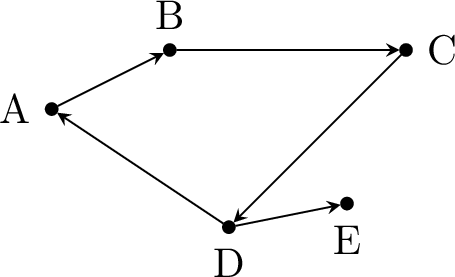
A directed graph (or digraph) contains arrows indicating the direction in which we can move along the arcs.

The in-degree is the number of arcs coming into the vertex.
The out-degree is the number of arcs going out from the vertex.

A loop (an arc from a vertex to itself) counts once in the in-degree and once in the out-degree of that vertex.

Example

In this graph, there is an arc from A to B, but no arc from B to A.

Definition — Subgraph

A subgraph is a graph that is made from a subset of the vertices and edges of another graph.

Definition — Simple Graph

A graph is called simple if it contains no loops and if there is a maximum of one edge joining any pair of distinct vertices.

Definition — Complete Graph

A complete graph is a simple undirected graph in which every vertex is connected by an edge to every other vertex.
The notation $K_n$ is used to describe the complete graph with $n$ vertices.

Skills to practice

Determining the Degree of Vertices

I.2 Walks and Connectedness

Recappreviously studied — click to reread

Definition — Walk, Trail, Path, Circuit and Cycle

A walk is a sequence of vertices such that each successive pair is adjacent.
A trail is a walk in which no edge is repeated.
A path is a walk in which no vertex is repeated.
A circuit is a trail that starts and ends at the same vertex (a closed trail).
A cycle is a circuit in which no vertex is repeated except the first, which is also the last.

Example

In this graph:

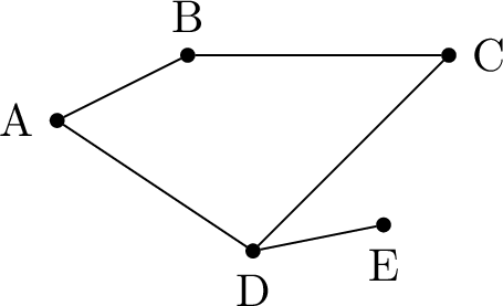
$A\rightarrow B\rightarrow C$ is a walk because there is an edge between $A$ and $B$ and an edge between $B$ and $C$.
$A\rightarrow B\rightarrow A$ is not a trail because the edge between $A$ and $B$ is repeated.
$A\rightarrow B\rightarrow C\rightarrow D\rightarrow A$ is not a path because the vertex $A$ is repeated.
$A\rightarrow B\rightarrow C\rightarrow D\rightarrow A$ is a circuit (and a cycle).

Definition — Connected Graph

A graph is called connected if it is possible to travel from any vertex to any other vertex via a sequence of edges.
The separate pieces of a graph that is not connected are its connected components.

Definition — Strongly Connected Graph

A directed graph is strongly connected if it is possible to travel from any vertex to any other vertex by following the directions of the arcs.
For undirected graphs, being connected is enough; strong connectivity is the directed analogue.

Skills to practice

Walks and Connectedness

I.3 Weighted Graphs

Recappreviously studied — click to reread

Definition — Weighted Graph

A weighted graph has numbers assigned to its edges. These numbers may represent the cost, time, or distance.

Skills to practice

Weighted Graphs

II Adjacency Matrices

II.1 Adjacency Matrix

Definition — Adjacency Matrix

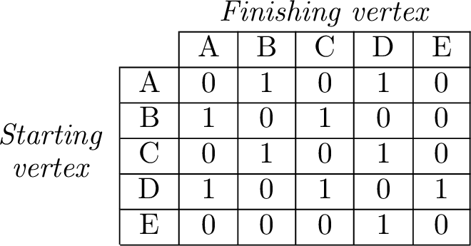
For a graph with $n$ vertices, the adjacency matrix $\mathbf{M}$ is an $n \times n$ matrix where the element $m_{ij}$ represents the number of direct edges from vertex $i$ to vertex $j$.

Example

The table below shows the number of 1-step walks between the vertices:

The adjacency matrix for the graph is therefore:$$ \mathbf{M} = \begin{pmatrix}0 & 1 & 0 & 1 & 0 \\ 1 & 0 & 1 & 0 & 0 \\ 0 & 1 & 0 & 1 & 0 \\ 1 & 0 & 1 & 0 & 1 \\ 0 & 0 & 0 & 1 & 0\end{pmatrix} $$ Since we do not usually write the labels for the vertices on the adjacency matrix, it is important to remember what the rows and columns refer to. To make this easier, we put them in alphabetical order.

Skills to practice

Checking Properties of Adjacency Matrices
Writing Adjacency Matrices

II.2 Matrix Powers with Technology

Recappreviously studied — click to reread

Method — Matrix Calculations with Technology

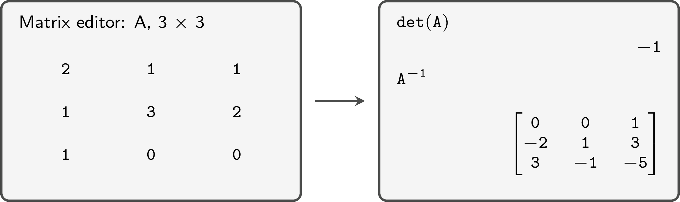
The matrix editor of a graphing calculator stores matrices under names ($\mathbf{A}$, $\mathbf{B}$, …); the main screen then calculates with these names.

Enter each matrix: choose its name, give its size (number of rows $\times$ number of columns), then type the entries row by row, each with its sign.
Write the calculation on the main screen with the stored names: $\mathbf{A} + \mathbf{B}$, $\mathbf{A} - \mathbf{B}$, $k\mathbf{A}$, $\mathbf{A}\mathbf{B}$, $\mathbf{A}^n$, $\det(\mathbf{A})$ (in the matrix menu) and $\mathbf{A}^{-1}$ (with the key $x^{-1}$).
Read the result entry by entry. When an exact answer is asked, convert the decimal entries into fractions with the fraction command, then check them exactly (step 5); round only the final answers.
Interpret an error message. A dimension error means that the operation is not defined for these sizes, for instance $\mathbf{A}\mathbf{B}$ when the number of columns of $\mathbf{A}$ differs from the number of rows of $\mathbf{B}$. A singular matrix error means that the square matrix has no inverse.
Check a result that matters: one entry of a product, row by column; for an inverse given with exact fractions, the product $\mathbf{A}\mathbf{A}^{-1}$ with these fractions must be exactly $\mathbf{I}$ (at least one row checked by hand).

The calculator also gives the determinant of a square matrix of order $3$ or more. It plays the same role as for order $2$ (admitted here): the matrix is invertible if and only if its determinant is not zero. The mock-up enters $\mathbf{A} = \begin{pmatrix} 2 & 1 & 1 \\ 1 & 3 & 2 \\ 1 & 0 & 0 \end{pmatrix}$, then computes $\det(\mathbf{A}) = -1 \neq 0$ and the inverse, whose entries here are whole numbers.

Skills to practice

Matrix Powers with Technology

II.3 Number of Walks of a Given Length

Proposition — Multi-step Walks

If $\mathbf{M}$ is the adjacency matrix, then the element $(i,j)$ of $\mathbf{M}^k$ gives the number of walks of length $k$ from vertex $i$ to vertex $j$.

Proof

We prove the statement by induction on the length $k$.
Base case $k=1$. By definition of the adjacency matrix, the element $(i,j)$ of $\mathbf{M}^1 = \mathbf{M}$ is the number of edges joining vertex $i$ to vertex $j$, which is exactly the number of walks of length $1$ from $i$ to $j$.
Induction step. Assume that for some $k \geq 1$, the element $(i,l)$ of $\mathbf{M}^k$ counts the walks of length $k$ from $i$ to $l$, for all vertices $i$ and $l$.
A walk of length $k+1$ from $i$ to $j$ is a walk of length $k$ from $i$ to some intermediate vertex $l$, followed by one edge from $l$ to $j$. For a fixed intermediate vertex $l$, the number of such walks is the product $(\mathbf{M}^k)_{il} \times m_{lj}$. Summing over all possible intermediate vertices: $$\begin{aligned}[t] \text{number of walks of length } k+1 \text{ from } i \text{ to } j &= \sum_{l} (\mathbf{M}^k)_{il} \, m_{lj} && \text{(count per intermediate vertex)} \\ &= (\mathbf{M}^k \mathbf{M})_{ij} && \text{(definition of the matrix product)} \\ &= (\mathbf{M}^{k+1})_{ij}. \end{aligned}$$ By induction, the result holds for every length $k \geq 1$.

Example

To understand why the powers of $\mathbf{M}$ count the multi-step walks, consider $\mathbf{M}^2$: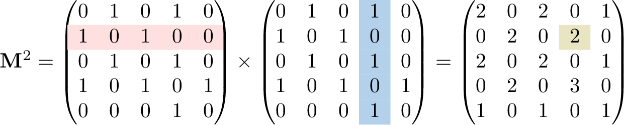

The element in row 2 column 4 of $\mathbf{M}^2$ shows there are two 2-step walks from B to D.
This value comes from the multiplication row 2 $\times$ column 4 as follows:

$1 \times 1 = 1$ walk from B to A $\times$ 1 walk from A to D
$0 \times 0 = 0$ walks from B to B $\times$ 0 walks from B to D
$1 \times 1 = 1$ walk from B to C $\times$ 1 walk from C to D
$0 \times 0 = 0$ walks from B to D $\times$ 0 walks from D to D
$0 \times 1 = 0$ walks from B to E $\times$ 1 walk from E to D

Adding these terms gives the two 2-step walks from B to D. The walks are $\text{B} \rightarrow \text{A} \rightarrow \text{D}$ and $\text{B} \rightarrow \text{C} \rightarrow \text{D}$.

Proposition — Walks of Bounded Length

Let $\mathbf{M}$ be the adjacency matrix of a graph and $k \geq 1$ a whole number. The element $(i,j)$ of $$\mathbf{S}_k = \mathbf{M} + \mathbf{M}^2 + \cdots + \mathbf{M}^k$$ gives the number of walks from vertex $i$ to vertex $j$ whose length is at least $1$ and at most $k$ (in a directed graph, the walks follow the arrows).
In particular, for $i \neq j$, the element $(i,j)$ of $\mathbf{S}_k$ is $0$ exactly when vertex $j$ cannot be reached from vertex $i$ in $k$ steps or fewer.

Proof

A walk of length at most $k$ has exactly one length $\ell$, with $1 \leq \ell \leq k$: the walks of different lengths are different walks, so their numbers add up. By the Multi-step Walks property, there are $(\mathbf{M}^{\ell})_{ij}$ walks of length $\ell$ from $i$ to $j$. Hence $$\begin{aligned}[t] \text{number of walks of length } 1 \text{ to } k &= (\mathbf{M})_{ij} + (\mathbf{M}^2)_{ij} + \cdots + (\mathbf{M}^k)_{ij} && \text{(sum over the lengths)} \\ &= (\mathbf{M} + \mathbf{M}^2 + \cdots + \mathbf{M}^k)_{ij} && \text{(sum of matrices, element by element)} \\ &= (\mathbf{S}_k)_{ij}. \end{aligned}$$ For $i \neq j$, this number is $0$ exactly when no walk of at most $k$ steps leads from $i$ to $j$, that is when $j$ cannot be reached from $i$ in $k$ steps or fewer.

Example

The one-way bus lines between four villages $P$, $Q$, $R$ and $S$ are shown below.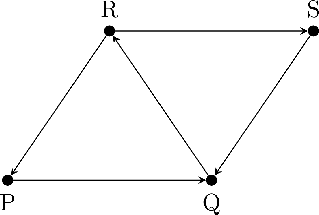

Write the adjacency matrix $\mathbf{M}$ and calculate $\mathbf{M} + \mathbf{M}^2$. Which villages cannot be reached from which with at most two bus rides?
Using technology, calculate $\mathbf{M} + \mathbf{M}^2 + \mathbf{M}^3$ and interpret the result.

Solution.

With the vertex order $P, Q, R, S$ (rows: departure, columns: arrival), and $\mathbf{M}^2$ obtained row by column: $$\mathbf{M} = \begin{pmatrix} 0 & 1 & 0 & 0 \\ 0 & 0 & 1 & 0 \\ 1 & 0 & 0 & 1 \\ 0 & 1 & 0 & 0 \end{pmatrix}, \qquad \mathbf{M}^2 = \begin{pmatrix} 0 & 0 & 1 & 0 \\ 1 & 0 & 0 & 1 \\ 0 & 2 & 0 & 0 \\ 0 & 0 & 1 & 0 \end{pmatrix},$$ $$\mathbf{M} + \mathbf{M}^2 = \begin{pmatrix} 0 & 1 & 1 & 0 \\ 1 & 0 & 1 & 1 \\ 1 & 2 & 0 & 1 \\ 0 & 1 & 1 & 0 \end{pmatrix}.$$ Outside the leading diagonal, the elements $(P,S)$ and $(S,P)$ are $0$: with at most two rides, $S$ cannot be reached from $P$, and $P$ cannot be reached from $S$. Every other village can be reached from every other one.
Technology gives $$\mathbf{M} + \mathbf{M}^2 + \mathbf{M}^3 = \begin{pmatrix} 1 & 1 & 1 & 1 \\ 1 & 2 & 1 & 1 \\ 1 & 2 & 2 & 1 \\ 1 & 1 & 1 & 1 \end{pmatrix}.$$ No element is $0$: every village can be reached from every other one with at most three rides. For instance, the element $(P,S)$ is $1$: the walk $P \to Q \to R \to S$.

The elements count walks, which may pass through a vertex twice: the element $(Q,Q)$ of $\mathbf{M}^3$ is $2$, for the round trips $Q \to R \to P \to Q$ and $Q \to R \to S \to Q$. To know the routes themselves, we list them on the graph.

Skills to practice

Interpreting Powers of the Adjacency Matrix
Counting Walks of Bounded Length
Determining the Number of Walks

II.4 Weighted Adjacency Tables

Definition — Weighted Adjacency Table

Let a weighted simple graph (no loop, at most one edge between two vertices) have its vertices listed in a fixed order. Its weighted adjacency table has one row and one column for each vertex: the entry in row $i$ and column $j$ is the weight of the edge joining $i$ to $j$ (a cost, a distance, a time), and a dash (—) shows that there is no such edge.
For an undirected graph, the table is symmetric about its leading diagonal: each edge appears twice, once in the row of each of its two endpoints.

Example

The weighted graph below shows the lengths, in kilometres, of the roads between five hamlets.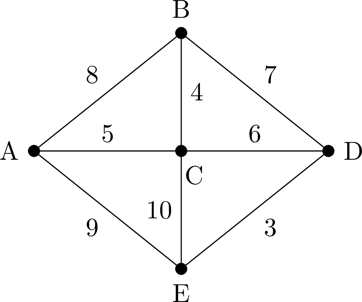

Write the weighted adjacency table of the graph.
Read the degree of $C$ and the total length of the roads from the table.

Solution.

Each edge gives two entries, one in the row of each endpoint:

A B C D E

A — 8 5 — 9

B 8 — 4 7 —

C 5 4 — 6 10

D — 7 6 — 3

E 9 — 10 3 —

The table is symmetric about its leading diagonal, as the graph is undirected.
The row of $C$ has $4$ entries ($5$, $4$, $6$, $10$), one for each edge at $C$: $\deg(C) = 4$.
Each road appears twice in the table, so we add the entries above the leading diagonal only: $$\begin{aligned}[t] \text{total length} &= (8 + 5 + 9) + (4 + 7) + (6 + 10) + 3 && \text{(rows } A, B, C, D \text{, above the diagonal)} \\ &= 22 + 11 + 16 + 3 \\ &= 52 \text{ km}. \end{aligned}$$

Skills to practice

Reading Weighted Adjacency Tables

II.5 Transition Matrix of a Graph

Adjacency matrices also let us study random walks on a graph: a token sits on a vertex and, at each step, moves along one of the edges at that vertex, each edge being equally likely. Random walks model a web surfer clicking links at random, a board-game piece, or a molecule moving through a network of cells.

Report an error

Definition — Transition Matrix of a Graph

Consider a random walk on a connected simple graph (strongly connected if the graph is directed), where at each step the token leaves the current vertex along one of its edges (or arcs), all equally likely.
The transition matrix $\mathbf{T}$ of the graph is the square matrix where the entry $t_{ij}$ is the probability of moving to vertex $i$ from vertex $j$:

$t_{ij} = \dfrac{1}{\deg(j)}$ if an edge joins $j$ to $i$ (in a digraph: an arc from $j$ to $i$, and $\deg(j)$ = out-degree of $j$);
$t_{ij} = 0$ otherwise.

Each column of $\mathbf{T}$ sums to $1$: the columns represent the current vertex (From), the rows the next vertex (To), matching the convention used for Markov chains.

Method — Constructing the Transition Matrix

Find the degree (out-degree for a digraph) of each vertex.
Fill column $j$: write $\dfrac{1}{\deg(j)}$ in each row $i$ such that an edge (or arc) goes from $j$ to $i$; write $0$ elsewhere.
Check that every column sums to $1$.

Example

A token performs a random walk on the following graph, starting at $A$.

The degrees are $\deg(A)=1$, $\deg(B)=2$, $\deg(C)=1$. From $A$ the token must move to $B$; from $B$ it moves to $A$ or $C$ with probability $\frac{1}{2}$ each; from $C$ it must move to $B$. With the vertex order $A, B, C$: $$\mathbf{T} = \begin{pmatrix} 0 & \frac{1}{2} & 0 \\ 1 & 0 & 1 \\ 0 & \frac{1}{2} & 0 \end{pmatrix}$$ We record the position probabilities in a column state vector $\mathbf{s}_n$; the initial state is $\mathbf{s}_0 = \begin{pmatrix} 1 \\ 0 \\ 0 \end{pmatrix}$. Then: $$\mathbf{s}_1 = \mathbf{T}\mathbf{s}_0 = \begin{pmatrix} 0 \\ 1 \\ 0 \end{pmatrix} \qquad \text{and} \qquad \mathbf{s}_2 = \mathbf{T}\mathbf{s}_1 = \begin{pmatrix} \frac{1}{2} \\ 0 \\ \frac{1}{2} \end{pmatrix}.$$ After one step the token is certainly at $B$; after two steps it is at $A$ or at $C$, each with probability $\frac{1}{2}$.

The long-run behaviour of a random walk — the proportion of time spent at each vertex — is studied with the tools of Markov chains: the walk is a Markov chain whose transition matrix is the one defined above. For a connected undirected graph, the long-run proportions are proportional to the degrees of the vertices: the token spends more time at the best-connected vertices.

Report an error

Skills to practice

Constructing the Transition Matrix of a Graph

III Trees and Minimum Spanning Trees

III.1 Trees and Spanning Trees

Definition — Tree

A tree is a connected graph with no cycles.

Example

Some examples of trees are shown below: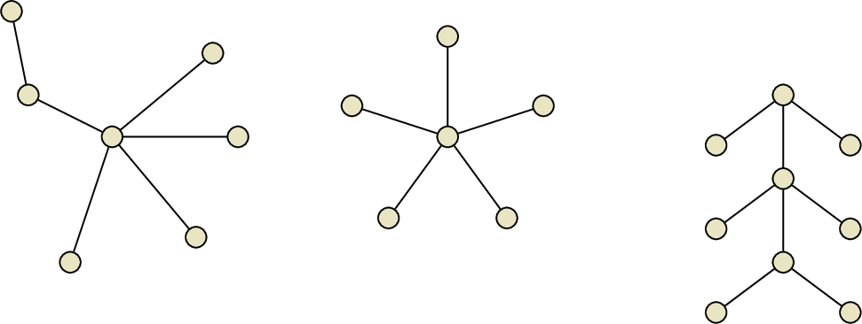

Definition — Spanning Tree

A spanning tree of a connected graph is a subgraph that contains all the vertices of the original graph and is a tree (connected and with no cycles).

Example

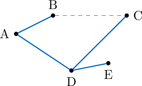
Consider the following graph $G$:

This graph has a cycle ($A-B-C-D-A$). To form a spanning tree, we must remove an edge to break the cycle while keeping all vertices connected.
For instance, if we remove the edge connecting $B$ and $C$, we get a spanning tree (highlighted in blue):

Skills to practice

Identifying Trees

III.2 Minimum Spanning Trees

Definition — Minimum Spanning Tree

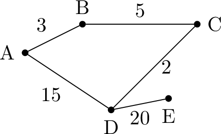
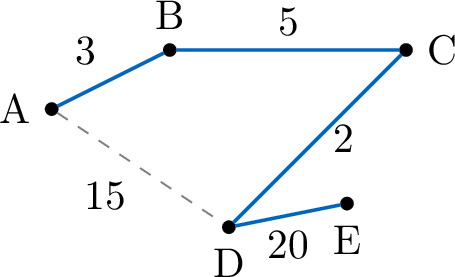
For a weighted connected graph, a minimum spanning tree (MST) is a spanning tree where the sum of the weights of the edges is minimised. It connects all vertices with the lowest possible total cost.

Example

Consider the weighted graph below. The Minimum Spanning Tree is:

The total weight of the Minimum Spanning Tree is $20 + 2 + 3 + 5 = 30$.

Method — Prim's Algorithm for MST

Start with any vertex.
Choose the edge with the lowest weight connecting a vertex in the tree to a vertex outside.
Add the chosen edge and the new vertex. Repeat until all vertices connected.

Example

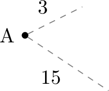
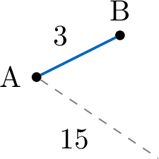
We apply Prim's algorithm to this graph.

Start at A. The edges connected to A are AB (3) and AD (15).
Choose AB (weight 3) as it is the lowest. Our tree is $\{A, B\}$.
Look at the edges connecting $\{A, B\}$ to the outside: AD (15) and BC (5).
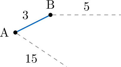
Choose BC (weight 5). Our tree is $\{A, B, C\}$.
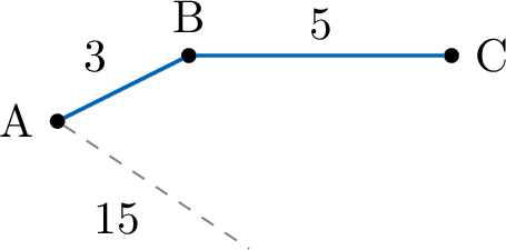
Look at the edges connecting $\{A, B, C\}$ to the outside: AD (15) and CD (2).
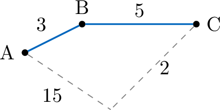
Choose CD (weight 2). Our tree is $\{A, B, C, D\}$.
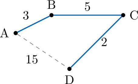
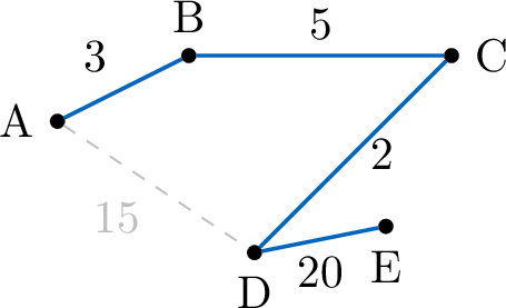
Look at the edges connecting $\{A, B, C, D\}$ to the outside: DE (20). Note that AD is now an internal edge (both endpoints are in the tree), so we ignore it.
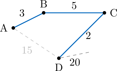
Choose DE (weight 20).

All vertices are connected. Total weight: $3 + 5 + 2 + 20 = 30$.

Method — Kruskal's Algorithm for MST

List (or sort) all edges in non-decreasing order of weight.
Start with an empty set of selected edges (a forest of isolated vertices).
Consider edges in that order. For each edge, add it if it connects two different components (i.e. it does not create a cycle); otherwise skip it.
Stop when $n-1$ edges have been selected (equivalently, when all $n$ vertices are connected).

Example

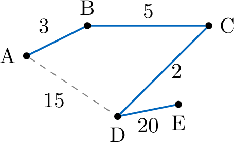
We apply Kruskal's algorithm to the same graph.

List all edges by weight (ascending):
- CD (2)
- AB (3)
- BC (5)
- AD (15)
- DE (20)
Select edges in order:
- Select CD (weight 2). No cycle.
- Select AB (weight 3). No cycle.
- Select BC (weight 5). No cycle.
- Consider AD (weight 15). Adding this edge would form a cycle ($A-B-C-D-A$). Reject.
- Select DE (weight 20). No cycle.

The algorithm stops when $n-1$ edges are selected (here, 4 edges).

Total weight: $2 + 3 + 5 + 20 = 30$.

Method — Prim's Algorithm on a Weighted Adjacency Table

Prim's algorithm can be run on the weighted adjacency table of a connected undirected graph, without drawing the graph:

Choose a starting vertex. Cross out its row and label its column $1$.
In the labelled columns, look at the entries that lie in rows not yet crossed out, and circle the smallest (if several are equal, choose any of them).
The circled entry joins the vertex of its column, already in the tree, to the vertex of its row, which is new: add this edge. Cross out the row of the new vertex and label its column with the next number.
Repeat steps 2 and 3 until every row is crossed out. The circled entries are the edges of a minimum spanning tree, and their sum is its weight.

The crossed-out rows are the vertices already in the tree, and the entries of the labelled columns in the other rows are the edges that leave the tree: each step adds the cheapest edge joining the tree to a new vertex, which is Prim's rule.

Example

The table gives the lengths, in kilometres, of the roads between five hamlets. Apply Prim's algorithm to the table, starting at $A$, to find a minimum spanning tree.

	A	B	C	D	E
A	—	8	5	—	9
B	8	—	4	7	—
C	5	4	—	6	10
D	—	7	6	—	3
E	9	—	10	3	—

Solution.

Start at $A$: cross out row $A$, label column $A$ with $1$. Column $A$, rows $B$ to $E$: $8$, $5$, —, $9$. The smallest is $5$, in row $C$: edge $AC$ ($5$).
Cross out row $C$, label column $C$ with $2$. Columns $A$ and $C$, rows $B$, $D$, $E$: $8$, —, $9$ and $4$, $6$, $10$. The smallest is $4$ (column $C$, row $B$): edge $CB$ ($4$).
Cross out row $B$, label column $B$ with $3$. Columns $A$, $C$, $B$, rows $D$, $E$: —, $9$; $6$, $10$; $7$, —. The smallest is $6$ (column $C$, row $D$): edge $CD$ ($6$).
Cross out row $D$, label column $D$ with $4$. Row $E$ in the labelled columns: $9$, $10$, —, $3$. The smallest is $3$ (column $D$): edge $DE$ ($3$).
Cross out row $E$, label column $E$ with $5$: every row is crossed out.

The table with its labels and the circled entries shown in colour:

	1	3	2	4	5
	A	B	C	D	E
A	—	8	5	—	9
B	8	—	4	7	—
C	5	4	—	6	10
D	—	7	6	—	3
E	9	—	10	3	—

The minimum spanning tree has the edges $AC$, $CB$, $CD$, $DE$, and its weight is $$5 + 4 + 6 + 3 = 18 \text{ km}.$$ Check with Kruskal's algorithm: the edges sorted by weight begin with $DE$ ($3$), $BC$ ($4$), $AC$ ($5$), $CD$ ($6$), and none of them closes a cycle: the same tree.

Skills to practice

Optimising Networks
Determining the Minimum Spanning Tree
Applying Prim's Algorithm to a Table

IV Eulerian Graphs

IV.1 Eulerian Trails and Circuits

Recappreviously studied — click to reread

Definition — Eulerian Graphs

An Eulerian circuit is a trail which traverses every edge of the graph exactly once and starts and ends at the same vertex.
An Eulerian trail traverses every edge exactly once but starts and ends at different vertices.

Proposition — Conditions for Eulerian Graphs

A connected undirected graph has an Eulerian circuit if and only if every vertex has an even degree.
A connected undirected graph has an Eulerian trail if and only if it has exactly two vertices of odd degree.

Proof

The degrees are necessary. Follow an Eulerian circuit. Each time it passes through a vertex, it arrives along one edge and leaves along another; at the vertex where it starts and ends, the first edge and the last edge form one more such pair. The circuit uses every edge exactly once, so the edges at each vertex are grouped in pairs: every degree is even. For an Eulerian trail, the same pairing works at every vertex except the start, whose first edge is alone, and the end, whose last edge is alone; the start and the end are different, so exactly these two vertices have an odd degree. The degrees are sufficient for a circuit. Let the graph be connected, with every degree even. Start at any vertex $A$ that has an edge, and walk along edges not yet used, as long as possible. The walk can only stop at $A$: each time it enters another vertex, it has used an odd number of the edges at that vertex (two at each earlier passage, one now), and the degree is even, so an unused edge remains to leave by. The walk is therefore a circuit $C$ (a trail that ends where it starts). If $C$ uses every edge, it is an Eulerian circuit. Otherwise some vertex $B$ of $C$ still has an unused edge. Indeed, take an unused edge: if one of its ends lies on $C$, that end will do; if not, the graph being connected, a path joins one of its ends to $A$, and the first edge of that path with one end on $C$ and the other end off $C$ is unused (an edge of $C$ has both ends on $C$), and it touches $C$. At each vertex, $C$ uses an even number of edges, so among the unused edges every degree is still even: a walk from $B$ along unused edges closes at $B$, giving a circuit $C'$. Inserting $C'$ into $C$ at $B$ gives a longer circuit. Repeating, the number of edges used grows each time, and the graph has finitely many edges: the process ends with a circuit that uses every edge, an Eulerian circuit. The degrees are sufficient for a trail. Let the graph be connected with exactly two vertices of odd degree, $P$ and $Q$. Add a new vertex $X$ joined to $P$ and to $Q$. The new graph is connected, and every degree is even ($P$ and $Q$ gain one, $X$ has degree $2$), so it has an Eulerian circuit, which may be started at $X$: it reads $X \to P \to \cdots \to Q \to X$ or the reverse. Removing $X$ and its two edges leaves a trail from $P$ to $Q$ that uses every edge of the original graph exactly once: an Eulerian trail.

Example

Consider the following undirected graph (a “bowtie” shape).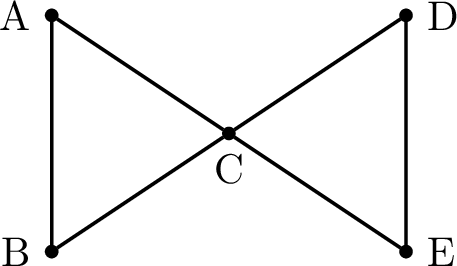

The degrees of the vertices (the number of edges connected to each) are:

$\deg(A) = 2$
$\deg(B) = 2$
$\deg(C) = 4$ (connected to A, B, D, E)
$\deg(D) = 2$
$\deg(E) = 2$

Since the graph is connected and all vertices have an even degree, the graph contains an Eulerian circuit.
One possible circuit is: $C \to A \to B \to C \to D \to E \to C$.

Skills to practice

Identifying Eulerian Circuits and Trails

IV.2 The Chinese Postman Problem

The Chinese Postman Problem was posed by the mathematician Kwan Mei-Ko. The problem asks: how can a postman deliver mail along every road in a network and return to the depot travelling the minimum possible distance?
Mathematically, this means traversing every edge of a weighted graph at least once and returning to the start.

Report an error

Method — The Chinese Postman Problem

The goal is to find the shortest closed walk that traverses every edge at least once.
If the graph is not Eulerian, we must repeat edges to make all vertices even-degree.

Identify all vertices with odd degrees.
Find all possible pairings of these odd vertices.
For each pair, find the shortest path between them.
Select the pairing that adds the minimum total weight.
Add this weight to the total weight of the graph.

Example

Solve the Chinese Postman Problem for the following weighted graph.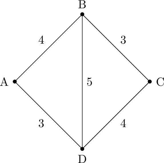

Total weight of the graph: $4+3+4+3+5 = 19$.
Identify odd degrees:
- $\deg(A)=2$, $\deg(C)=2$ (Even).
- $\deg(B)=3$, $\deg(D)=3$ (Odd).
The odd vertices are B and D.
Find shortest path between odd vertices: The odd vertices must be paired. Since there are only two, the pair is (B, D).
Paths from B to D:
- Direct: B $\to$ D (weight 5).
- Via A: B $\to$ A $\to$ D (weight $4+3=7$).
- Via C: B $\to$ C $\to$ D (weight $3+4=7$).
The shortest path is the direct edge BD with weight 5.
Calculate optimal distance: Total = Graph Weight + Shortest Path Addition Total = $19 + 5 = 24$.

To minimise distance, the postman must traverse the edge BD twice.
One possible optimal walk is:$$ A \to B \to D \to B \to C \to D \to A $$

Why the Pairing Works

A closed route arrives at a vertex as many times as it leaves it, so it uses an even number of edge-ends at every vertex. Travelling an edge a second time amounts to adding a copy of that edge to the graph. The copies must therefore make every vertex even: an odd number of copies meets at each odd vertex, so the copied edges can be split into routes that join the odd vertices in pairs (and possibly closed loops, which only add length, since the weights are positive). Replacing each of these routes by a shortest path between its two ends cannot increase the total, so an optimal route repeats shortest paths, and we compare the ways of pairing the odd vertices: with $2$ odd vertices there is $1$ pairing; with $4$ odd vertices $W$, $X$, $Y$, $Z$ there are $3$ pairings, $\{WX, YZ\}$, $\{WY, XZ\}$ and $\{WZ, XY\}$. With the copies of the best pairing, every degree is even: an Eulerian circuit exists, and it is an optimal route.
If the route may start and finish at different vertices, it is an Eulerian trail of the graph with its copies, so its two ends are the two vertices left odd. With $4$ odd vertices, the best choice takes two of them as the ends and joins only the other two by a shortest path: ending at an even vertex would leave at least one pair of odd vertices to join as well, which cannot cost less.

Report an error

Example

An inspector must walk along every path of the park shown below, starting and finishing at the entrance $A$. The lengths are in hundreds of metres.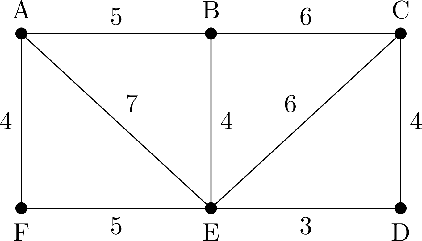

Find the length of the shortest route and the paths walked twice.
The inspector may now finish at any vertex. Where should the route end, and how long is it?

Solution.

The degrees are $\deg(A) = \deg(B) = \deg(C) = 3$, $\deg(D) = \deg(F) = 2$, $\deg(E) = 5$: the four odd vertices are $A$, $B$, $C$, $E$. The total length of the paths is $5+6+4+3+5+4+4+7+6 = 44$.
Shortest paths between odd vertices: $AB = 5$, $AC = 11$ (via $B$), $AE = 7$, $BC = 6$, $BE = 4$, $CE = 6$. The three pairings: $$\begin{aligned}[t] \{AB, CE\} &: 5 + 6 = \mathbf{11} \\ \{AC, BE\} &: 11 + 4 = 15 \\ \{AE, BC\} &: 7 + 6 = 13 \end{aligned}$$ The best pairing repeats the paths $AB$ and $CE$: $$44 + 11 = 55 \text{ hundreds of metres, i.e. } 5.5 \text{ km}.$$ One such route: $A \to B \to C \to D \to E \to C \to E \to B \to A \to F \to E \to A$.
The route starts at $A$, which is odd; the best choice ends it at another odd vertex, and the remaining two are joined by a shortest path: $$\begin{aligned}[t] \text{end at } B &: \text{repeat } CE,\ 44 + 6 = 50 \\ \text{end at } C &: \text{repeat } BE,\ 44 + 4 = \mathbf{48} \\ \text{end at } E &: \text{repeat } BC,\ 44 + 6 = 50 \end{aligned}$$ The route should end at $C$; it is $4.8$ km long, for instance $A \to F \to E \to A \to B \to E \to B \to C \to E \to D \to C$.

Skills to practice

Solving the Chinese Postman Problem

V Hamiltonian Graphs

V.1 Hamiltonian Paths and Cycles

Definition — Hamiltonian Cycle and Path

A Hamiltonian cycle is a cycle that visits every vertex of the graph exactly once.
A Hamiltonian path visits every vertex exactly once but does not necessarily return to the start.

Example

Consider the following graph.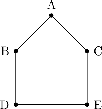

A Hamiltonian Path: $D \to B \to A \to C \to E$. (It visits every vertex exactly once, but does not return to $D$).
A Hamiltonian Cycle: $A \to B \to D \to E \to C \to A$. (It visits every vertex exactly once and returns to the start).

The Travelling Salesman Problem (TSP) describes a classic optimisation scenario: A salesman must leave his home town, visit a specific set of other towns exactly once, and then return home. The objective is to find the walk that minimises the total distance travelled.
In Graph Theory terms, this amounts to finding the Hamiltonian Cycle with the minimum total weight in a complete weighted graph.

Report an error

Skills to practice

Identifying Hamiltonian Paths and Cycles

V.2 The Travelling Salesman Problem

Method — The Travelling Salesman Problem (TSP)

The goal is to find the Hamiltonian cycle with the minimum total weight in a complete weighted graph.
Since finding the exact solution is hard, we find bounds:

Upper Bound (Nearest Neighbour Algorithm): Start at a vertex, always move to the nearest unvisited vertex, and return to the start at the end.
Lower Bound (Deleted Vertex Algorithm):
1. Delete a vertex $V$ and its edges.
2. Find the MST of the remaining graph.
3. Add the two shortest edges from $V$ to the MST weight.

Example

Find the bounds for the optimal tour starting at A for the following graph.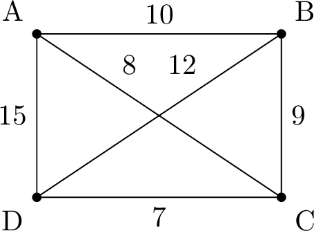

Upper Bound (Nearest Neighbour from A):
- Start at A. Nearest unvisited neighbours: B(10), C(8), D(15). Choose C.
- From C. Unvisited: B(9), D(7). Choose D.
- From D. Unvisited: B(12). Choose B.
- From B, return to start (A). Weight 10.
- Walk: $A \to C \to D \to B \to A$.
- Total Weight: $8 + 7 + 12 + 10 = 37$.
Lower Bound (Delete Vertex A):
- Remove A. Remaining vertices: B, C, D. Edges: BC(9), CD(7), BD(12).
- MST of remainder: Select CD(7), then BC(9). Total = 16.
- Edges from A: AB(10), AC(8), AD(15). Two shortest are 8 and 10.
- Total Weight: $16 + 8 + 10 = 34$.

The optimal solution is between 34 and 37.

Practical and Classical TSP

The TSP described above is the classical TSP: the graph is complete and each vertex is visited exactly once. In a real road network — the practical TSP — some towns are not directly connected, and the best route may pass through a town more than once.
To convert a practical problem into a classical one, we build the table of least distances: for every pair of vertices, we record the length of the shortest route between them (direct or through intermediate vertices). This table defines a complete weighted graph, on which the classical TSP is solved; an “edge” of the completed graph may represent a route through intermediate towns, which are then revisited in the real network.

Report an error

Example

Convert the following practical network into a complete graph using the table of least distances.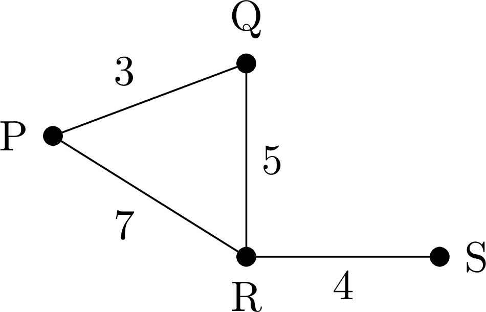

The pairs $P$–$S$ and $Q$–$S$ have no direct edge, so we compute their shortest routes:

$P \to S$: via $R$, $7 + 4 = 11$; via $Q$ and $R$, $3 + 5 + 4 = 12$. Shortest: $\mathbf{11}$.
$Q \to S$: via $R$, $5 + 4 = \mathbf{9}$.
$P \to R$: direct $7$; via $Q$, $3 + 5 = 8$. Shortest: the direct edge, $\mathbf{7}$.

	P	Q	R	S
P	—	3	7	11
Q	3	—	5	9
R	7	5	—	4
S	11	9	4	—

The classical TSP is now solved on this complete graph; the entry $P$–$S = 11$ means “travel through $R$”, so $R$ is revisited in the real network.

Skills to practice

Finding Optimal Tour Bounds

VI Going further

Skills to practice

Diagnosing and Correcting
Solving Problems with Graphs
Quiz

	1	3	2	4	5
	A	B	C	D	E
A	—	8	5	—	9
B	8	—	4	7	—
C	5	4	—	6	10
D	—	7	6	—	3
E	9	—	10	3	—

	1	3	2	4	5
	A	B	C	D	E
A	—	8	5	—	9
B	8	—	4	7	—
C	5	4	—	6	10
D	—	7	6	—	3
E	9	—	10	3	—

	1	3	2	4	5
	A	B	C	D	E
A	—	8	5	—	9
B	8	—	4	7	—
C	5	4	—	6	10
D	—	7	6	—	3
E	9	—	10	3	—