International Baccalaureate · DP 2: Applications and Interpretation HL

Hypothesis Testing

⌚ ~186 min ▢ 21 blocks ✓ 88 exercises ➣ Prerequisites : Estimation and Confidence Intervals

I The Logic of a Test

I.1 Null and Alternative Hypotheses

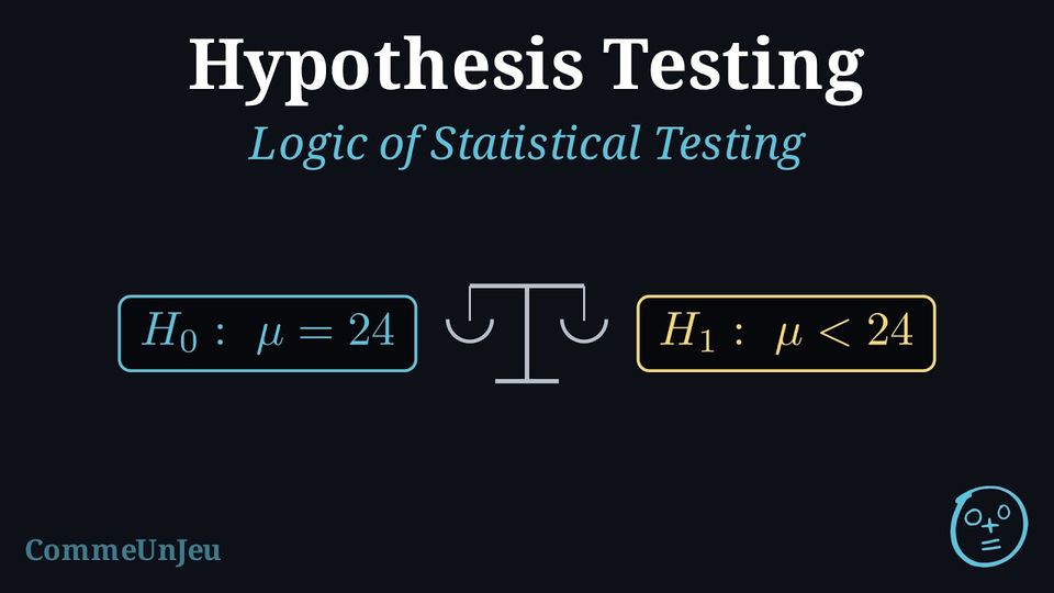
Statistical testing functions much like a court trial.

The Assumption (Innocence): We start by assuming there is no effect or no difference until proven otherwise.
The Evidence (Data): We collect data from a sample.
The Verdict: If the evidence is strong enough (beyond reasonable doubt), we reject the initial assumption.

Important: In hypothesis testing, we never “prove” $H_0$ is true. We either reject $H_0$ or fail to reject it because the evidence is not strong enough.

Report an error

Definition — Null and Alternative Hypotheses

The Null Hypothesis ($H_0$) represents the status quo, “no difference,” or “no effect.” For tests on a numerical parameter, it includes an equality ($\mu = k$, $\mu \leq k$, or $\mu \geq k$); for chi-squared tests, $H_0$ states independence or a given distribution.
The Alternative Hypothesis ($H_1$) is the claim we are trying to find evidence for. It uses strict inequalities ($\mu \neq k$, $\mu > k$, or $\mu < k$).

Example

A company claims that the average battery life of their new phone is 24 hours. A consumer group suspects the battery life is actually shorter. Write the null and alternative hypotheses.

Answer

Let $\mu$ be the true mean battery life.

$H_0: \mu = 24$ (The company's claim is true; there is no difference).
$H_1: \mu < 24$ (The consumer group's suspicion; the mean is less than claimed).

Skills to practice

Choosing the Hypotheses
Formulating Null and Alternative Hypotheses

I.2 p-value and Significance Level

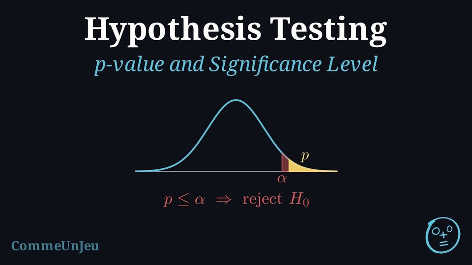
Definition — p-value and $\alpha$

The significance level ($\alpha$) is the threshold for evidence (usually $0.05$, $0.01$, or $0.10$). It is the maximum probability, accepted in advance, of rejecting $H_0$ when it is actually true (a Type I error).
The p-value is the probability of obtaining sample results at least as extreme as the ones observed, assuming $H_0$ is true.

A small p-value means the data would be very unlikely if $H_0$ were true, so it is evidence against $H_0$.
Decision Rule:

If $p\text{-value} \leq \alpha \implies$ Reject $H_0$. (The result is statistically significant).
If $p\text{-value} > \alpha \implies$ Fail to reject $H_0$. (Not enough evidence against $H_0$).

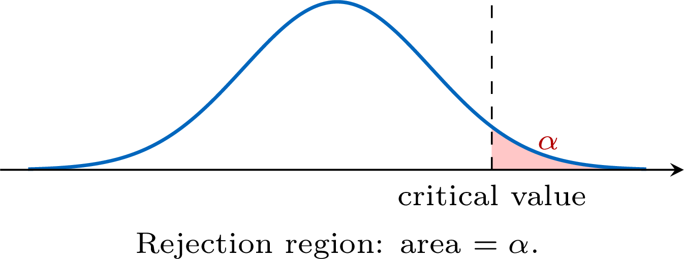
The decision rule has a clear visual meaning. If $H_0$ is true, the test statistic follows a known distribution. The p-value is the area in the tail beyond the observed statistic — the probability of a result at least as extreme. The rejection region is the set of most-extreme values whose total area is exactly $\alpha$. Rejecting $H_0$ when the statistic lands in the rejection region is the same decision as rejecting when the p-value is at most $\alpha$.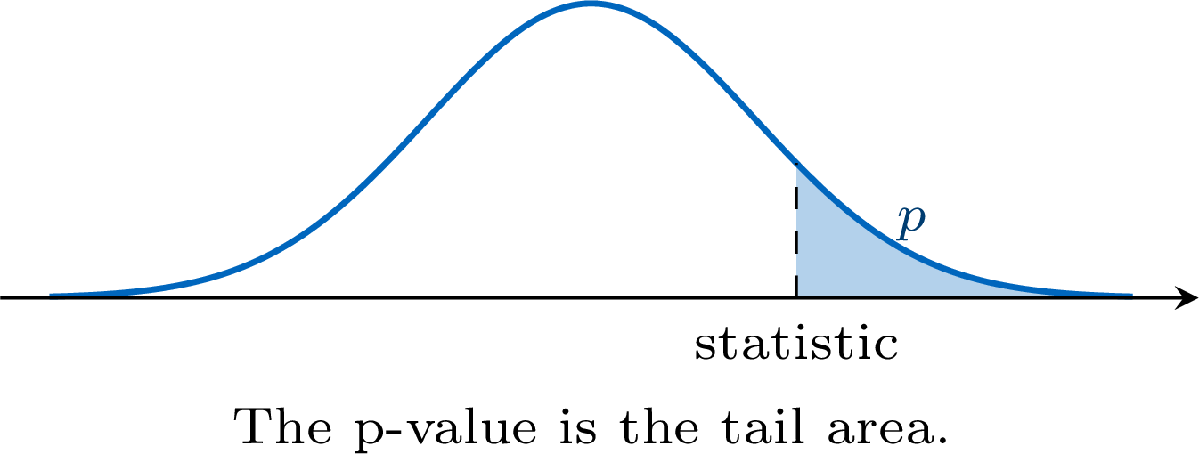

\hspace{0.4cm}

Report an error

Example

A researcher performs a hypothesis test to check if a new fertilizer increases plant growth.
The calculated $p$-value is $0.042$.
Make a conclusion for the following significance levels:

$\alpha = 0.05$ ($5\pourcent$ significance level).
$\alpha = 0.01$ ($1\pourcent$ significance level).

Answer

For $\alpha = 0.05$: $$ p\text{-value} = 0.042 < 0.05 $$ Since the $p$-value is smaller than $\alpha$, the result is statistically significant at the 5$\pourcent$ level. We reject the null hypothesis ($H_0$). There is sufficient evidence at the 5$\pourcent$ significance level to support the claim.
For $\alpha = 0.01$: $$ p\text{-value} = 0.042 \geq 0.01 $$ Since the $p$-value is greater than $\alpha$, the result is not statistically significant at this level. We fail to reject the null hypothesis ($H_0$). There is not enough evidence at the 1$\pourcent$ significance level to support the claim.

Skills to practice

Deciding from a p-value
Interpreting the p-value

I.3 The Five Steps of a Test

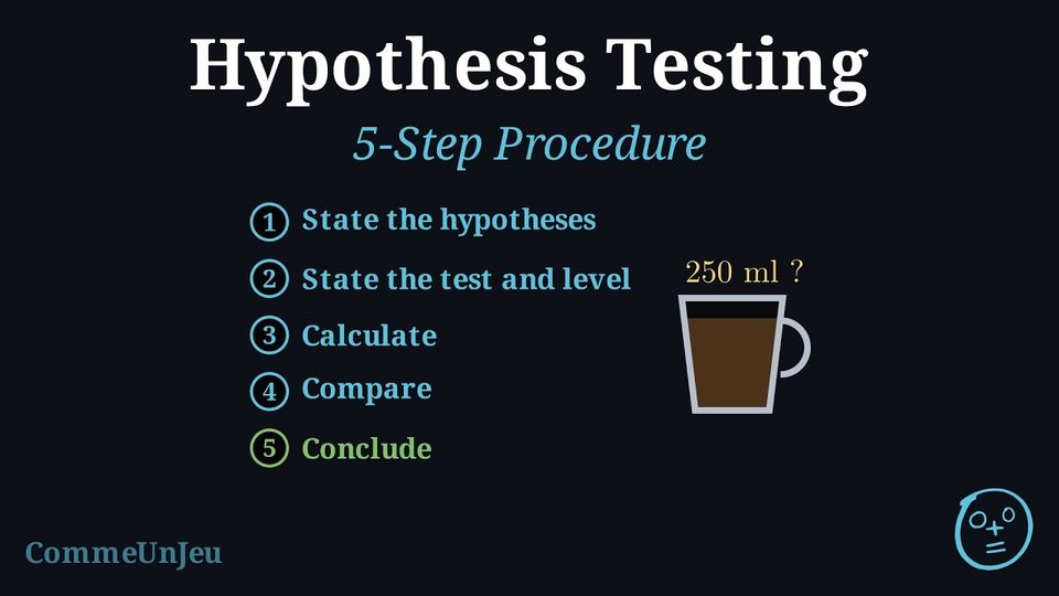
Method — Performing a Hypothesis Test

State the Hypotheses: Define the parameter (e.g., $\mu$) and write $H_0$ and $H_1$.
State the Test and Level: Identify the test (e.g., t-test) and the significance level $\alpha$.
Calculate Statistics: Use the GDC to find the test statistic and the p-value.
Compare: Explicitly compare the p-value to $\alpha$ (usually check whether $p \leq \alpha$ or $p > \alpha$).
Conclude: Write a conclusion in the context of the problem, referring to the original claim.

Example

(This example uses the one-sample t-test; the focus here is the five-step logic.)
A coffee machine is supposed to dispense $250$ ml per cup. A manager suspects it is dispensing less. He measures a sample of 10 cups and finds a mean of $\bar{x} = 248$ ml with a standard deviation of $s_{n-1} = 3$ ml.
Test the manager's suspicion at the $5\pourcent$ significance level.

Answer

Let $\mu$ be the population mean volume of coffee.

$H_0: \mu = 250$ and $H_1: \mu < 250$.
One-sample t-test at $\alpha = 0.05$.
Using GDC (T-Test with $\mu_0=250, \bar{x}=248, s=3, n=10, <\mu_0$):
$t \approx -2.108$ and $p\text{-value} \approx 0.032$.
Since $0.032 < 0.05$, we reject $H_0$.
There is sufficient evidence to suggest the machine is dispensing less than 250 ml.

Skills to practice

Identifying the Steps of a Hypothesis Test

I.4 Type I and Type II Errors

Definition — Error Types

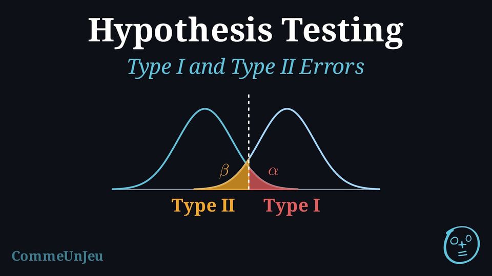
When making a decision based on a statistical test, there is always a risk of error.

Type I Error: Rejecting $H_0$ when $H_0$ is actually true (False Positive). When $H_0$ is true, this error is the event “reject $H_0$”; its probability is at most the significance level $\alpha$: equal to $\alpha$ for a $z$-test, and equal to the actual significance level of the test, which can be smaller than $\alpha$, for a binomial or a Poisson test.
Type II Error: Failing to reject $H_0$ when $H_0$ is actually false (False Negative). When $H_0$ is false, this error is the event “do not reject $H_0$”; its probability is denoted $\beta$.

	$H_0$ is True	$H_0$ is False
Reject $H_0$	Type I Error	Correct Decision
Fail to Reject $H_0$	Correct Decision	Type II Error

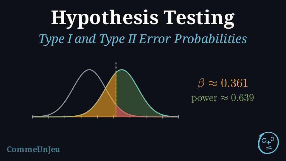
The two errors can be seen at once. The left curve is the distribution of the statistic when $H_0$ is true; the right curve when $H_0$ is false. The critical value (dashed) splits the axis into “reject” (right) and “do not reject” (left). The probability of a Type~I error is the area under the $H_0$ curve on the reject side ($\alpha$); the probability of a Type~II error is the area under the $H_1$ curve on the do-not-reject side ($\beta$). The event “reject $H_0$” is the same set of values of the statistic in both pictures; what changes from one curve to the other is the probability attached to it. Moving the critical value to shrink one area enlarges the other.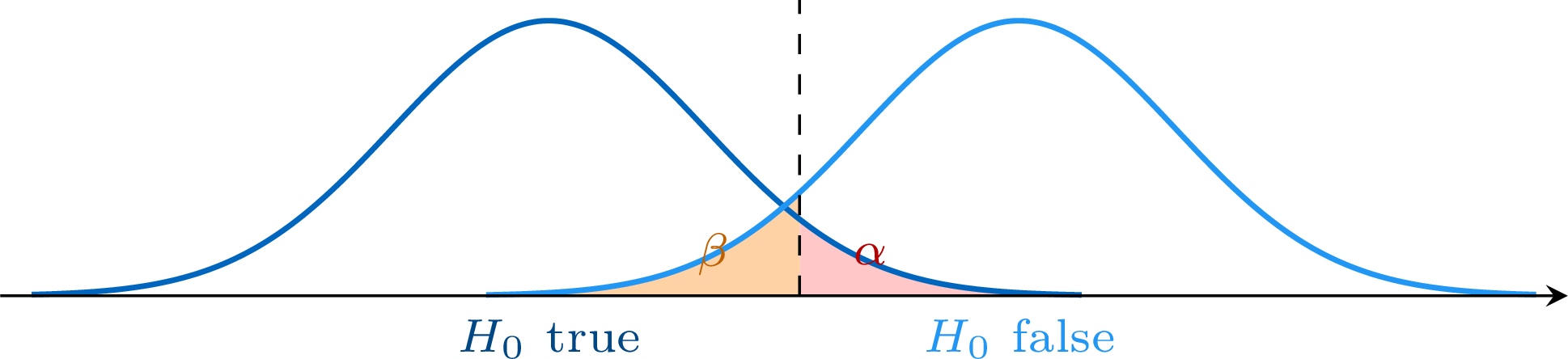

Report an error

Example

A factory produces parachutes. The null hypothesis states that a batch of parachutes is safe.

$H_0$: The parachutes are safe.
$H_1$: The parachutes are defective.

Describe the Type I and Type II errors. Which error is more dangerous in this context?

Answer

Type I Error: The inspector concludes the parachutes are defective (rejects $H_0$) when they are actually safe ($H_0$ is true). Consequence: Financial loss from stopping production or destroying good products.
Type II Error: The inspector concludes the parachutes are safe (fails to reject $H_0$) when they are actually defective ($H_0$ is false). Consequence: Potentially fatal accidents.

In this context, a Type II error is much more dangerous because human lives are at risk.

Skills to practice

Interpreting Type I and Type II Errors in Context

II The z-test and Critical Regions

II.1 The z-test for a Mean

When the Standard Deviation Is Known

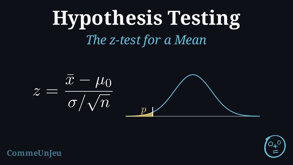
A test on a mean compares the mean $\bar{x}$ of a sample with the value $\mu_0$ that $H_0$ claims. How far $\bar{x}$ may fall from $\mu_0$ by chance alone depends on the spread of the population. Sometimes this spread is known: a filling machine whose standard deviation has been measured over years of production, or an instrument whose precision is certified, keeps its standard deviation $\sigma$ even when its mean drifts. Then the distribution of the sample mean needs no estimate of the spread. For a normal population, $\overline{X} \sim \mathcal{N}\left(\mu, \dfrac{\sigma^2}{n}\right)$ (sum and mean of normal variables); for any population and a large sample, $\overline{X}$ is approximately normal with the same parameters (central limit theorem). Standardising $\overline{X}$ with the value $\mu_0$ of $H_0$ gives a statistic whose distribution is known when $H_0$ is true: the standard normal distribution, exactly for a normal population and approximately for a large sample. When $\sigma$ is unknown, it is estimated from the sample, and the $t$-tests of the next section take over.

Report an error

Definition — The $z$-test for a Mean

A population has an unknown mean $\mu$ and a known standard deviation $\sigma$; the population is normal, or the sample is large (commonly $n \geq 30$, more when the population is strongly skewed). For a random sample of size $n$ with mean $\bar{x}$, the $z$-test of $H_0 : \mu = \mu_0$ uses the test statistic $$\textcolor{colordef}{z = \dfrac{\bar{x} - \mu_0}{\sigma / \sqrt{n}}},$$ which, when $H_0$ is true, is a value of $Z \sim \mathcal{N}(0, 1)$ (exactly for a normal population, approximately for a large sample). The p-value is a tail area of the standard normal distribution, in the direction of $H_1$:

$H_1$	$\mu > \mu_0$	$\mu < \mu_0$	$\mu \neq \mu_0$
$p\text{-value}$	$P(Z \geq z)$	$P(Z \leq z)$	$2\,P(Z \geq \|z\|)$

Method — Performing a $z$-test

Hypotheses: define $\mu$ in context, then write $H_0 : \mu = \mu_0$ and $H_1$, one-tailed ($\mu > \mu_0$ or $\mu < \mu_0$) when the question points in one direction, two-tailed ($\mu \neq \mu_0$) otherwise.
Conditions: check that $\sigma$ is known and that the population is normal or the sample large.
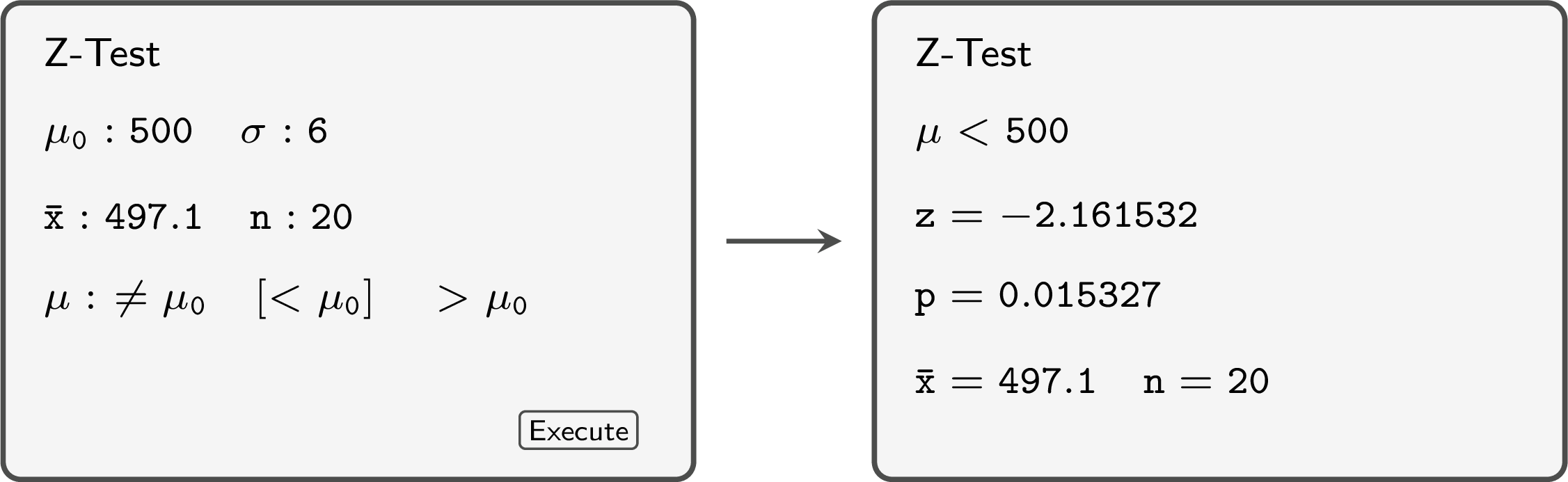
Statistic and p-value: compute $z = \dfrac{\bar{x} - \mu_0}{\sigma / \sqrt{n}}$, then the tail area with the normal cumulative distribution function of $\mathcal{N}(0, 1)$; or run the 1-sample $z$-test of the calculator (Z-Test), which takes $\mu_0$, $\sigma$, then $\bar{x}$ and $n$ (or the list of data) and the direction of $H_1$, and returns $z$ and the p-value.
Decision: reject $H_0$ if $p\text{-value} \leq \alpha$; otherwise do not reject it.
Conclusion: state what the decision means in the context of the question.

The mock-up shows the test of the next example: $\mu_0 = 500$, $\sigma = 6$, $\bar{x} = 497.1$, $n = 20$, $H_1 : \mu < 500$.

Example

The masses of the cereal boxes filled by a machine are normally distributed, with a standard deviation of $6$ g known from the long-run record of the machine. The boxes should contain $500$ g on average. After a repair, an inspector suspects that the mean mass has dropped. A random sample of $20$ boxes has a mean mass of $497.1$ g. Test the inspector's suspicion at the $5\pourcent$ significance level.

Answer

Let $\mu$ be the mean mass, in grams, of the boxes filled after the repair.

$H_0 : \mu = 500$ and $H_1 : \mu < 500$ (the suspicion points downwards: one-tailed test).
$\sigma = 6$ is known and the masses are normal: $z$-test at $\alpha = 0.05$.
With $\bar{x} = 497.1$ and $n = 20$: $$\begin{aligned}[t] z &= \frac{\bar{x} - \mu_0}{\sigma / \sqrt{n}} && \text{(test statistic of the } z\text{-test)} \\ &= \frac{497.1 - 500}{6 / \sqrt{20}} \\ &\approx \frac{-2.9}{1.3416} \approx -2.162, \end{aligned}$$ and $p\text{-value} = P(Z \leq -2.162) \approx 0.0153$ (the Z-Test of the calculator gives the same values).
$0.0153 \leq 0.05$: reject $H_0$.
At the $5\pourcent$ level, the data support the inspector: the mean mass of the boxes has dropped below $500$ g.

Skills to practice

Computing the z-statistic and the p-value
Performing a z-test

II.2 Critical Values and Critical Regions

Definition — Critical Region and Critical Value

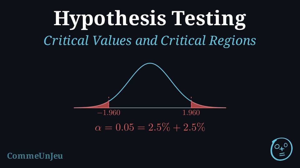
In a test at significance level $\alpha$:

the critical region is the set of values of the test statistic for which $H_0$ is rejected; the other values form the acceptance region, where $H_0$ is not rejected (which does not prove it);
a critical value is a boundary of the critical region.

For a $z$-test, the critical region is the tail, or the two tails, of $\mathcal{N}(0, 1)$ with total area $\alpha$, on the side of $H_1$. With $z_\alpha$ the number such that $P(Z \geq z_\alpha) = \alpha$:

$H_1$	$\mu > \mu_0$	$\mu < \mu_0$	$\mu \neq \mu_0$
critical region	$z \geq z_\alpha$	$z \leq -z_\alpha$	$z \leq -z_{\alpha/2}$ or $z \geq z_{\alpha/2}$

The statistic lies in the critical region exactly when the p-value is at most $\alpha$: the two ways of deciding always agree. The usual critical values are:

$\alpha$	$0.10$	$0.05$	$0.01$
one-tailed $z_\alpha$	$1.282$	$1.645$	$2.326$
two-tailed $z_{\alpha/2}$	$1.645$	$1.960$	$2.576$

Method — Finding a Critical Region

Critical value of $Z$: since $P(Z \leq z_\alpha) = 1 - \alpha$, the inverse normal function of the calculator with area $1 - \alpha$, $\mu = 0$ and $\sigma = 1$ gives $z_\alpha$; for a two-tailed test, the area is $1 - \dfrac{\alpha}{2}$.

Critical region for the sample mean: when $H_0$ is true, $\overline{X} \sim \mathcal{N}\left(\mu_0, \dfrac{\sigma^2}{n}\right)$ (exactly or approximately, as for $z$), so the critical region can be written directly for $\bar{x}$:

$\mu > \mu_0$	$\mu < \mu_0$	$\mu \neq \mu_0$
$\bar{x} \geq \mu_0 + z_\alpha\,\sigma/\sqrt{n}$	$\bar{x} \leq \mu_0 - z_\alpha\,\sigma/\sqrt{n}$	$\bar{x} \leq \mu_0 - z_{\alpha/2}\,\sigma/\sqrt{n}$ or $\bar{x} \geq \mu_0 + z_{\alpha/2}\,\sigma/\sqrt{n}$

The inverse normal function with mean $\mu_0$ and standard deviation $\dfrac{\sigma}{\sqrt{n}}$ gives these bounds in one step.

Decision: reject $H_0$ if the observed value lies in the critical region.

Example

A machine fills bottles with a volume that is normally distributed with standard deviation $12$ ml. The mean volume is set at $1000$ ml. Each morning, a random sample of $36$ bottles is measured to check that the setting has not moved in either direction, at the $5\pourcent$ significance level.

Find the critical region of the test for the mean volume $\bar{x}$ of the sample.
One morning, $\bar{x} = 1003.1$ ml. What is the decision?

Answer

Let $\mu$ be the mean volume, in ml: $H_0 : \mu = 1000$, $H_1 : \mu \neq 1000$, a two-tailed test.

The standard deviation of $\overline{X}$ is $\dfrac{\sigma}{\sqrt{n}} = \dfrac{12}{\sqrt{36}} = 2$, and $z_{0.025} \approx 1.960$ (inverse normal with area $0.975$). The critical values are $$\begin{aligned}[t] \mu_0 \pm z_{\alpha/2}\,\frac{\sigma}{\sqrt{n}} &= 1000 \pm 1.960 \times 2 && \text{(critical region for } \bar{x}\text{)} \\ &= 1000 \pm 3.92, \end{aligned}$$ so the critical region is $\bar{x} \leq 996.08$ or $\bar{x} \geq 1003.92$.
$996.08 < 1003.1 < 1003.92$: the observed mean is not in the critical region, so $H_0$ is not rejected: at the $5\pourcent$ level, there is not enough evidence that the setting has moved. Check with the statistic: $z = \dfrac{1003.1 - 1000}{2} = 1.55$ and $|1.55| < 1.960$, the p-value being $2\,P(Z \geq 1.55) \approx 0.121 > 0.05$.

Skills to practice

Finding Critical Values and Critical Regions

III The t-test

III.1 The One-Sample t-test

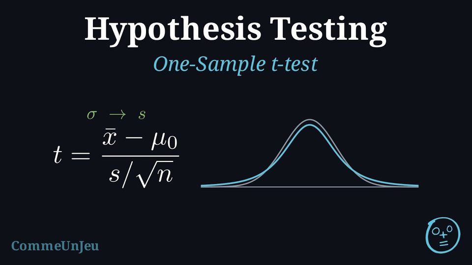
The t-test is one of the most commonly used statistical tests. It is used to determine if there is a significant difference between means, especially when the population variance is unknown and the sample size is small ($n < 30$).

Report an error

Definition — One-Sample t-test Formula

The one-sample t-test compares the mean of a single sample ($\bar{x}$) to a known or hypothesized population mean ($\mu_0$).
It is used when:

The data come from a random sample of quantitative (continuous) values.
The population follows a normal distribution (or the sample size is large, commonly $n \geq 30$, so that the distribution of $\bar{x}$ is approximately normal).
The population standard deviation $\sigma$ is unknown (we use the unbiased sample standard deviation $s = s_{n-1}$, the $s_x$ key of calculators).

The test statistic $t$ is calculated as:$$ t = \frac{\bar{x} - \mu_0}{s / \sqrt{n}} $$

Method — Steps for a One-Sample t-test using Calculator

Step 1: Write the Hypotheses
- $H_0: \mu = k$ (The population mean equals a specific value $k$).
- $H_1: \mu \neq k$ (or $\mu < k$, $\mu > k$ depending on the question).
Step 2: Enter data into GDC
- Enter the data into List 1 (or use summary statistics $\bar{x}, s, n$).
- Select T-Test (or 1-Sample t-test).
- Enter the value of $\mu_0$ (from $H_0$).
Step 3: Decision Rule
Compare the p-value with the significance level $\alpha$.
- If $p\text{-value} < \alpha$: Reject $H_0$.
- If $p\text{-value} \geq \alpha$: Fail to reject $H_0$.
Step 4: Conclusion
State whether there is sufficient evidence to support the alternative hypothesis, in context.

Example

A factory produces screws with a target length of 50 mm. A quality control manager takes a random sample of 15 screws and finds a mean length of 49.8 mm with a standard deviation of 0.5 mm.
Conduct a t-test at the 5$\pourcent$ significance level to see if the mean length is different from 50 mm.

Answer

Step 1: Hypotheses
- $H_0: \mu = 50$ (The mean is 50 mm).
- $H_1: \mu \neq 50$ (The mean is different from 50 mm).
Step 2: Calculator
Using GDC with inputs: $\mu_0=50, \bar{x}=49.8, s_x=0.5, n=15$. $$ t \approx -1.549 $$ $$ p\text{-value} \approx 0.144 $$
Step 3: Decision
$0.144 > 0.05$. Since $p > \alpha$, we fail to reject $H_0$.
Step 4: Conclusion
There is insufficient evidence at the 5$\pourcent$ level to claim that the mean length of the screws is different from 50 mm.

Skills to practice

Conducting One-Sample t-tests

III.2 The Two-Sample t-test

Definition — Two-Sample t-test Formula

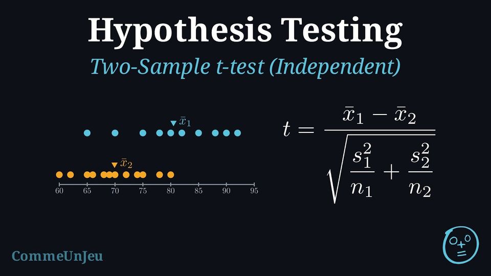
The two-sample t-test compares the means of two independent groups to see if they are significantly different.The test statistic is given by:$$ t = \frac{\bar{x}_1 - \bar{x}_2}{\sqrt{\frac{s_1^2}{n_1} + \frac{s_2^2}{n_2}}} $$ Where:

$\bar{x}_1, \bar{x}_2$ are the sample means.
$s_1^2, s_2^2$ are the sample variances.
$n_1, n_2$ are the sample sizes.

Assumptions: both groups are independent random samples from (approximately) normal populations, or both sample sizes are large. The calculator computes the degrees of freedom of this statistic automatically.

Definition — Pooled Two-Sample t-test

When the two independent samples come from normal populations with the same unknown variance $\sigma^2$, both samples estimate this one variance, and the pooled estimate combines them, each weighted by its number of degrees of freedom: $$\textcolor{colordef}{s_p^2 = \dfrac{(n_1 - 1)\,s_1^2 + (n_2 - 1)\,s_2^2}{n_1 + n_2 - 2}},$$ where $s_1^2$ and $s_2^2$ are the unbiased sample variances (computed with $n - 1$, the $s_x$ key of calculators squared). The pooled two-sample $t$-test of $H_0 : \mu_1 = \mu_2$ uses the statistic $$\textcolor{colordef}{t = \dfrac{\bar{x}_1 - \bar{x}_2}{s_p\sqrt{\dfrac{1}{n_1} + \dfrac{1}{n_2}}}},$$ which, when $H_0$ is true, follows the $t$-distribution with $n_1 + n_2 - 2$ degrees of freedom. On a calculator, it is the 2-sample $t$-test with the setting Pooled: Yes. The equal-variance assumption is made when the question states it, when a course or an examination sets it as the convention, or when the context makes it a reasonable modelling choice (two groups measured in the same way, with close sample standard deviations, which support it without proving it); otherwise, the unpooled statistic of the two-sample $t$-test is used.

Example

Seedlings of the same variety are grown with two nutrient solutions, $A$ and $B$, in two independent random samples. Their heights after four weeks, in cm, are:

solution $A$: $24.1$, $25.3$, $23.8$, $26.0$, $24.7$, $25.5$;
solution $B$: $22.9$, $23.5$, $24.0$, $22.4$, $23.8$, $23.1$, $24.2$.

Assuming that the heights are normally distributed with the same variance for both solutions, test at the $5\pourcent$ significance level whether solution $A$ gives a greater mean height.

Answer

Let $\mu_A$ and $\mu_B$ be the mean heights, in cm, with each solution.

$H_0 : \mu_A = \mu_B$ and $H_1 : \mu_A > \mu_B$ (one-tailed).
Normal populations with a common variance: pooled two-sample $t$-test at $\alpha = 0.05$.
From the lists: $\bar{x}_A = 24.9$, $s_A^2 = 0.724$ ($n_A = 6$); $\bar{x}_B \approx 23.414$, $s_B^2 \approx 0.4181$ ($n_B = 7$). $$\begin{aligned}[t] s_p^2 &= \frac{(n_A - 1)\,s_A^2 + (n_B - 1)\,s_B^2}{n_A + n_B - 2} && \text{(pooled estimate)} \\ &\approx \frac{5 \times 0.724 + 6 \times 0.4181}{11} \approx 0.5571, \\ t &= \frac{\bar{x}_A - \bar{x}_B}{s_p\sqrt{\frac{1}{n_A} + \frac{1}{n_B}}} && \text{(pooled statistic)} \\ &\approx \frac{24.9 - 23.414}{0.7464 \times 0.5563} \approx 3.58, \end{aligned}$$ with $6 + 7 - 2 = 11$ degrees of freedom. The calculator (2-sample $t$-test, Pooled: Yes, $\mu_1 > \mu_2$) gives $t \approx 3.578$ and $p\text{-value} \approx 0.00217$.
$0.00217 \leq 0.05$: reject $H_0$.
At the $5\pourcent$ level, the data show that solution $A$ gives taller seedlings on average.

Skills to practice

Conducting Pooled Two-Sample t-tests

III.3 The Paired t-test

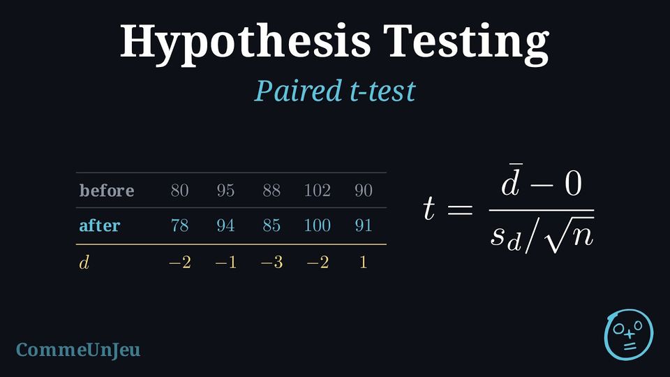
Definition — Paired t-test

The paired t-test compares the means of two dependent groups (e.g., “Before and After” measurements on the same subject or matched pairs).
It is used when:

The data consist of matched pairs $(x_1, x_2)$.
The differences $d = x_2 - x_1$ (or $x_1 - x_2$) are calculated.
The differences follow a normal distribution.

The test is essentially a one-sample t-test performed on the differences $d$, testing if the mean difference $\mu_d$ is zero.The test statistic is:$$ t = \frac{\bar{d} - 0}{s_d / \sqrt{n}} $$

Method — Steps for a Paired t-test

Step 1: Calculate Differences
Calculate the difference for each pair: $d_i = x_{2i} - x_{1i}$ (be consistent with the chosen order).
Step 2: Write the Hypotheses
Let $\mu_d$ be the population mean of the differences.
- $H_0: \mu_d = 0$ (No difference on average).
- $H_1: \mu_d \neq 0$ (or $\mu_d < 0$, $\mu_d > 0$).
Step 3: Enter data into GDC
- Enter the calculated differences into List 1 (or put raw data in L1, L2 and define L3 = L2 - L1).
- Select T-Test (1-Sample t-test) on the differences list.
- Set $\mu_0 = 0$.
Step 4: Decision and Conclusion
Compare the p-value to $\alpha$ and conclude in context.

Example

A weight-loss programme claims to reduce weight after one month. The weights of 5 participants are recorded before and after the programme.

Participant	1	2	3	4	5
Before (kg)	80	95	88	102	90
After (kg)	78	94	85	100	91

Test at the 5$\pourcent$ level if the programme effectively reduces weight.

Answer

Calculate Differences ($d = \text{After} - \text{Before}$): $$ d = \{78-80, 94-95, 85-88, 100-102, 91-90\} $$ $$ d = \{-2, -1, -3, -2, 1\} $$
Hypotheses:
Let $\mu_d$ be the mean difference.
- $H_0: \mu_d = 0$ (The programme has no effect).
- $H_1: \mu_d < 0$ (The programme reduces weight on average).
Calculator:
Perform a 1-Sample T-Test on the list of differences $\{-2, -1, -3, -2, 1\}$ with $\mu_0 = 0$ and test $< \mu_0$. $$ \bar{d} = -1.4, \quad s_d \approx 1.517 $$ $$ t \approx -2.06 $$ $$ p\text{-value} \approx 0.0540 $$
Conclusion:
$0.0540 > 0.05$. Since $p > \alpha$, we fail to reject $H_0$.
There is insufficient evidence at the 5$\pourcent$ level to conclude that the programme effectively reduces weight (although the mean difference is negative, the sample is small and the result is not statistically significant).

Skills to practice

Conducting Paired t-tests

III.4 Testing with a Confidence Interval

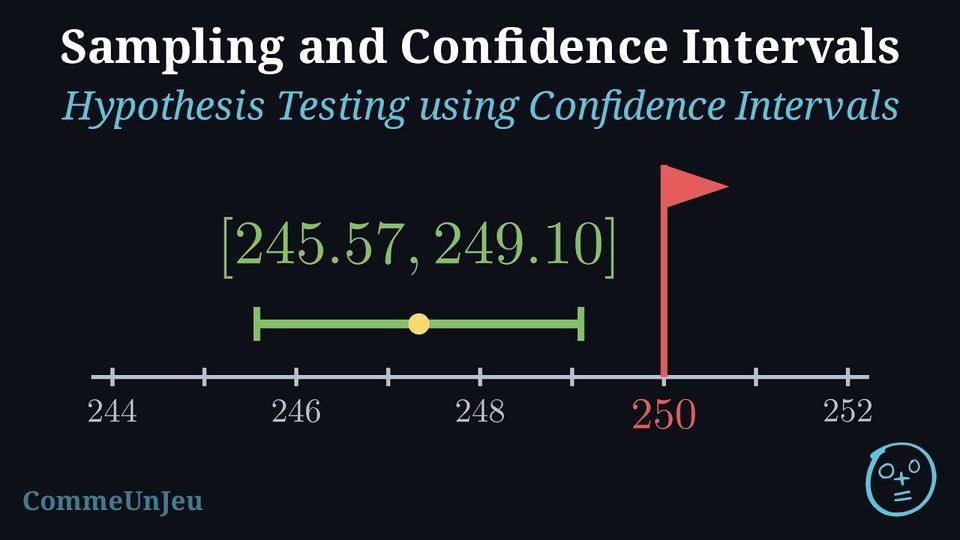
Confidence intervals can be used as a tool for hypothesis testing. If someone claims that the population mean is a specific value ($\mu_H$), we can check if this value is “plausible” by seeing whether it falls within our calculated confidence interval.
For a two-sided test at significance level $\alpha$ (e.g.\ $5\pourcent$), the $(1-\alpha)$ confidence interval (e.g.\ $95\pourcent$) gives the same decision as the corresponding hypothesis test $H_0 : \mu = \mu_H$ versus $H_1 : \mu \neq \mu_H$.

Report an error

Method — Hypothesis Test with CI

To test a claim that the population mean is $\mu_H$ at a significance level $\alpha$ (e.g., $5\pourcent$):

Construct the corresponding $(1-\alpha)$ confidence interval (e.g., $95\pourcent$) for $\mu$ based on sample data.
Decision rule:
- If $\mu_H$ is inside the interval, we do not reject the claim (the claim is plausible).
- If $\mu_H$ is outside the interval, we reject the claim (the result is statistically significant at level $\alpha$).

Example

A dairy states that its cartons contain $250$ ml of juice on average. A consumer group measures the contents, in millilitres, of $12$ cartons chosen at random: $$247, \ 251, \ 244, \ 249, \ 246, \ 250, \ 243, \ 248, \ 245, \ 252, \ 246, \ 247.$$ The contents are assumed to be normally distributed. Test the dairy's claim at the $5\pourcent$ significance level, using a $95\pourcent$ confidence interval for the mean content $\mu$.

Answer

The claim is $\mu = 250$; the test is two-sided ($H_1 : \mu \neq 250$), at the level $\alpha = 0.05$ that matches a $95\pourcent$ interval.

The population is normal and $\sigma$ is unknown: $t$-interval with $11$ degrees of freedom. With a calculator, $\bar{x} \approx 247.333$, $s_n \approx 2.7743$ and $t^* \approx 2.2010$, so $$E = t^* \frac{s_n}{\sqrt{n}} \approx 2.2010 \times \frac{2.7743}{\sqrt{12}} \approx 1.763,$$ and the interval is approximately $[245.57, 249.10]$ ml.
The claimed value $250$ lies outside the interval: the claim is rejected at the $5\pourcent$ level.
At the $5\pourcent$ level, the data show that the mean content of the cartons differs from $250$ ml; the interval suggests it is lower, between about $245.6$ ml and $249.1$ ml.

Skills to practice

Testing a Claim with a t-Interval

IV Tests for a Proportion and a Poisson Mean

IV.1 Test for a Proportion

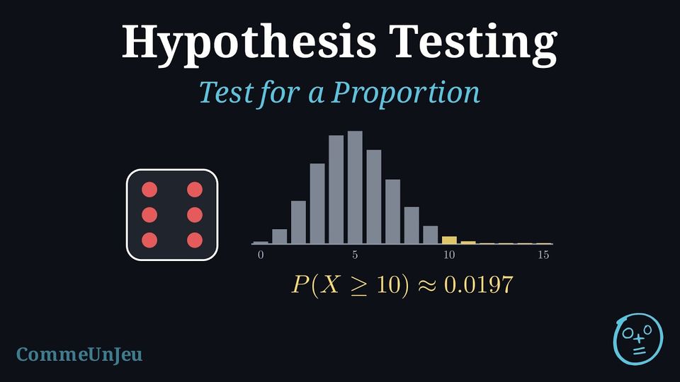
Testing with a Count

Some claims are about a proportion: the share of seeds that germinate, the probability that a die shows a six, the proportion of voters who support a candidate. A sample then gives a count: the number $X$ of successes among $n$ independent trials. If $H_0$ fixes the proportion at $p_0$, the distribution of $X$ is known exactly, $X \sim \mathcal{B}(n, p_0)$, and the count itself serves as the test statistic. Unlike a normal statistic, $X$ takes only whole values: its tail probabilities go up by jumps, so a set of extreme values can rarely have a probability of exactly $\alpha$. The critical region is the largest set of extreme values whose probability does not exceed $\alpha$, and that probability, the chance of rejecting $H_0$ when it is true, is the actual significance level of the test. The same reasoning applies to counts of events, modelled by a Poisson distribution.

Report an error

Definition — Test for a Proportion

Let $p$ be the probability of success in each of $n$ independent trials (or the proportion of successes in a population, sampled at random with a sample small compared with the population, so that the draws can be treated as independent), and $X$ the number of successes. The binomial test of $H_0 : p = p_0$ is one-tailed, against $H_1 : p > p_0$ or $H_1 : p < p_0$; when $H_0$ is true, $X \sim \mathcal{B}(n, p_0)$. For an observed count $x$:

$H_1$	$p > p_0$	$p < p_0$
$p\text{-value}$	$P(X \geq x)$	$P(X \leq x)$
critical region	$X \geq c$	$X \leq c$
choice of $c$	smallest $c$ with $P(X \geq c) \leq \alpha$	largest $c$ with $P(X \leq c) \leq \alpha$

The probability of the critical region under $H_0$ is the actual significance level: it is at most $\alpha$, and as close to $\alpha$ as the whole values of $X$ allow.

Method — Finding the Critical Region of a Discrete Test

When $H_0$ is true, $X \sim \mathcal{B}(n, p_0)$ or $X \sim \mathcal{P}(\lambda_0)$. The cumulative function of the calculator (binomcdf, poissoncdf) gives $P(X \leq k)$; a table of its values for $k = 0, 1, 2, \dots$ settles the region.

Lower tail ($H_1$ points down): read $P(X \leq k)$ in the table; $c$ is the last value of $k$ for which $P(X \leq k) \leq \alpha$, so that $P(X \leq c) \leq \alpha < P(X \leq c + 1)$.
Upper tail ($H_1$ points up): use $P(X \geq k) = 1 - P(X \leq k - 1)$; $c$ is the first value of $k$ for which $P(X \geq k) \leq \alpha$, so that $P(X \geq c) \leq \alpha < P(X \geq c - 1)$.
Actual level: report $P(X \leq c)$ or $P(X \geq c)$, the probability of the critical region under $H_0$.
Decision: reject $H_0$ if the observed count lies in the critical region — the same decision as $p\text{-value} \leq \alpha$.

If even the most extreme value has a probability greater than $\alpha$, the critical region is empty: with so few trials, the test can never reject $H_0$.

Example

A player suspects that a die shows a six more often than a fair die would. In $30$ rolls, it shows $10$ sixes. Test the player's suspicion at the $5\pourcent$ significance level.

Answer

Let $p$ be the probability that the die shows a six, and $X$ the number of sixes in $30$ rolls.

$H_0 : p = \dfrac{1}{6}$ (fair die) and $H_1 : p > \dfrac{1}{6}$.
The rolls are independent trials: under $H_0$, $X \sim \mathcal{B}\left(30, \dfrac{1}{6}\right)$; binomial test at $\alpha = 0.05$.
The observed count is $10$, and $H_1$ points up: $$\begin{aligned}[t] p\text{-value} &= P(X \geq 10) && \text{(upper tail)} \\ &= 1 - P(X \leq 9) \\ &\approx 1 - 0.9803 \approx 0.0197. \end{aligned}$$
$0.0197 \leq 0.05$: reject $H_0$.
At the $5\pourcent$ level, the data support the player: this die shows a six more often than a fair die. ($10$ sixes in $30$ rolls is twice the $5$ expected from a fair die.)

Example

A supplier states that $90\pourcent$ of its seeds germinate. A gardener suspects that the proportion is lower, and sows $40$ seeds to test the claim at the $5\pourcent$ significance level.

Find the critical region of the test and its actual significance level.
$33$ seeds germinate. What does the gardener conclude?

Answer

Let $p$ be the germination probability of a seed, and $X$ the number of the $40$ seeds that germinate: $H_0 : p = 0.9$, $H_1 : p < 0.9$, and under $H_0$, $X \sim \mathcal{B}(40, 0.9)$.

$H_1$ points down: the critical region is $X \leq c$, with $c$ the largest value such that $P(X \leq c) \leq 0.05$. The cumulative function gives:

$k$ $31$ $32$ $33$

$P(X \leq k)$ $0.0155$ $0.0419$ $0.0995$

$P(X \leq 32) \leq 0.05 < P(X \leq 33)$, so the critical region is $X \leq 32$, and the actual significance level is $P(X \leq 32) \approx 0.0419$.
$33$ is not in the critical region: $H_0$ is not rejected (equivalently, $p\text{-value} = P(X \leq 33) \approx 0.0995 > 0.05$). At the $5\pourcent$ level, the gardener has not shown that fewer than $90\pourcent$ of the seeds germinate.

Skills to practice

Finding Binomial p-values and Critical Regions
Testing a Proportion

IV.2 Test for a Poisson Mean

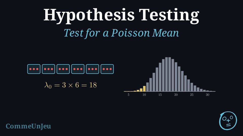
Definition — Test for a Poisson Mean

Events occur independently, one at a time, at a uniform average rate, and their number $X$ in an interval of observation is modelled by a Poisson distribution, $X \sim \mathcal{P}(\lambda)$, with $\lambda$ the mean number of events in that interval. The Poisson test of $H_0 : \lambda = \lambda_0$ is one-tailed, against $H_1 : \lambda > \lambda_0$ or $H_1 : \lambda < \lambda_0$. When $H_0$ is true, $X \sim \mathcal{P}(\lambda_0)$, where $\lambda_0$ is the mean for the whole interval of observation: a rate of $3$ events per month observed for $6$ months gives $\lambda_0 = 18$. The p-value, $P(X \geq x)$ or $P(X \leq x)$, and the critical region are found as for a proportion.

Example

Over many years, a road junction has had $3$ accidents per month on average, a record long enough for this rate to be treated as known. Traffic lights are then installed, and in the next $6$ months there are $10$ accidents. Assuming that accidents occur independently at a uniform rate, test at the $5\pourcent$ significance level whether the rate of accidents has decreased, then give the critical region of the test.

Answer

Let $\lambda$ be the mean number of accidents in $6$ months with the traffic lights, and $X$ the number of accidents in these $6$ months.

The old rate gives $\lambda_0 = 3 \times 6 = 18$: $H_0 : \lambda = 18$ and $H_1 : \lambda < 18$.
Under $H_0$, $X \sim \mathcal{P}(18)$; Poisson test at $\alpha = 0.05$.
$H_1$ points down: $p\text{-value} = P(X \leq 10) \approx 0.0304$ (cumulative function).
$0.0304 \leq 0.05$: reject $H_0$.
At the $5\pourcent$ level, the rate of accidents has decreased since the lights were installed.

Critical region: $P(X \leq 10) \approx 0.0304 \leq 0.05$ and $P(X \leq 11) \approx 0.0549 > 0.05$, so it is $X \leq 10$, with an actual significance level of $0.0304$; the observed $10$ lies in it, as the p-value showed.

Skills to practice

Finding Poisson p-values and Critical Regions
Testing a Poisson Mean

V Probabilities of Errors

V.1 Type I and Type II Error Probabilities

Definition — Probabilities of Errors and Power

For a test with critical region $C$:

The probability of a Type I error is the probability that the statistic lies in $C$ when $H_0$ is true. It equals $\alpha$ for a $z$-test, and the actual significance level, at most $\alpha$, for a binomial or Poisson test.
The probability $\beta$ of a Type II error is the probability that the statistic does not lie in $C$ when $H_1$ is true. Since $H_1$ allows many values of the parameter, $\beta$ is computed for one given value of the parameter under $H_1$.
The power of the test for that value is $1 - \beta$, the probability of rejecting $H_0$ when it is false.

For a fixed sample size, a smaller $\alpha$ gives a critical region that is no larger, hence a $\beta$ that is no smaller. A larger sample lowers $\beta$ at the same $\alpha$ for a $z$-test; for a discrete test, the jumps of the critical region can break this for one extra trial, but a substantially larger sample lowers $\beta$.

Method — Calculating Error Probabilities

Critical region: write it for the observed statistic, $\bar{x}$ for a $z$-test, the count $X$ for a binomial or Poisson test.
Type I error: its probability is that of the critical region under $H_0$: $\alpha$, or the actual significance level.
Type II error: take the distribution given by the stated value under $H_1$ — $\overline{X} \sim \mathcal{N}\left(\mu_1, \dfrac{\sigma^2}{n}\right)$, $X \sim \mathcal{B}(n, p_1)$ or $X \sim \mathcal{P}(\lambda_1)$ — and compute the probability that the statistic falls outside the critical region.
Interpretation: say in context what each error would mean and how likely it is.

Example

Bags of rice are filled with masses that are normally distributed with standard deviation $8$ g. The target mean is $500$ g, and overfilling costs money: each day, $16$ bags are weighed to test $H_0 : \mu = 500$ against $H_1 : \mu > 500$ at the $5\pourcent$ significance level.

Find the critical region for the mean mass $\bar{x}$ of the sample, and the probability of a Type I error.
The machine drifts to a mean of $504$ g. Find the probability of a Type II error, and the power of the test.

Answer

The standard deviation of $\overline{X}$ is $\dfrac{8}{\sqrt{16}} = 2$, and $z_{0.05} \approx 1.645$: $$\begin{aligned}[t] \mu_0 + z_\alpha\,\frac{\sigma}{\sqrt{n}} &\approx 500 + 1.6449 \times 2 && \text{(upper critical region)} \\ &\approx 503.29, \end{aligned}$$ so the critical region is $\bar{x} \geq 503.29$. For a $z$-test, $P(\text{Type I error}) = \alpha = 0.05$: on $5\pourcent$ of the days when the machine is well set, it is wrongly adjusted.
When $\mu = 504$, $\overline{X} \sim \mathcal{N}(504, 2^2)$, and a Type II error is a sample mean outside the critical region: $$\begin{aligned}[t] \beta &= P(\overline{X} < 503.29) && \text{(acceptance region, under } \mu = 504\text{)} \\ &= P\left(Z < \frac{503.29 - 504}{2}\right) \\ &\approx P(Z < -0.355) \approx 0.361. \end{aligned}$$ The power is $1 - \beta \approx 0.639$: a drift of $4$ g is missed on about $36\pourcent$ of the days.

Example

In the germination test of the previous section ($40$ seeds, $H_0 : p = 0.9$, $H_1 : p < 0.9$, $\alpha = 0.05$), the critical region is $X \leq 32$.

Find the probability of a Type I error.
In fact, only $80\pourcent$ of the seeds germinate. Find the probability of a Type II error, and interpret it.

Answer

Under $H_0$, $X \sim \mathcal{B}(40, 0.9)$ and $P(\text{Type I error}) = P(X \leq 32) \approx 0.0419$, the actual significance level, below $\alpha = 0.05$.
Now $X \sim \mathcal{B}(40, 0.8)$, and a Type II error is a count outside the critical region: $$\begin{aligned}[t] \beta &= P(X \geq 33) && \text{(acceptance region, under } p = 0.8\text{)} \\ &= 1 - P(X \leq 32) \\ &\approx 1 - 0.5629 \approx 0.437. \end{aligned}$$ Although the supplier's claim is false, the gardener has a probability of about $0.437$ of not rejecting it: $40$ seeds are too few to detect reliably a germination rate of $80\pourcent$ instead of $90\pourcent$.

Skills to practice

Calculating Error Probabilities
Interpreting Error Probabilities

VI Testing a Correlation Coefficient

VI.1 Testing $\rho \equal 0$

Definition — Pearson's Correlation Coefficient ($r$)

The Pearson's correlation coefficient ($r$) is a value in the range $[-1, 1]$ that quantifies the direction and strength of a linear relationship between two quantitative variables.

The sign of $r$ indicates the direction (positive or negative).
The magnitude (absolute value) of $r$ indicates the strength. An $|r|$ value close to 1 implies a strong linear correlation, while a value close to 0 implies a weak or no linear correlation.

Value of $\|r\|$	Strength of Correlation
$\|r\| = 1$	Perfect
$0.9 \le \|r\| < 1$	Very Strong
$0.7 \le \|r\| < 0.9$	Strong
$0.5 \le \|r\| < 0.7$	Moderate
$0.3 \le \|r\| < 0.5$	Weak
$0 \le \|r\| < 0.3$	Very Weak or None

A Correlation in a Sample

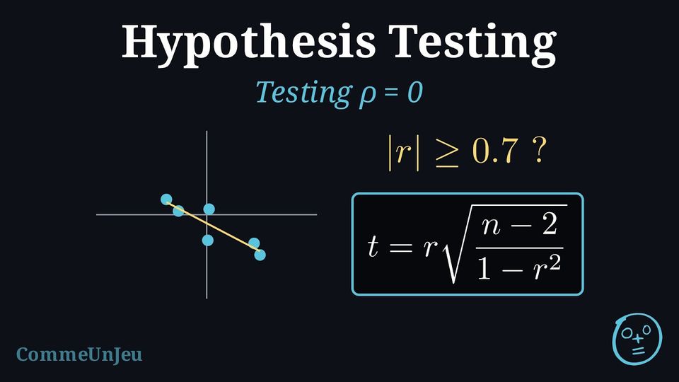
Pearson's coefficient $r$ measures the linear correlation of a sample of pairs. The same coefficient computed on every pair of the population is written $\rho$ (“rho”). A sample can show a strong $r$ even when $\rho = 0$: for two independent normal variables, a sample of $6$ pairs gives $|r| \geq 0.7$ about $12\pourcent$ of the time, a sample of $20$ pairs less than $0.1\pourcent$ of the time. Whether an observed $r$ is evidence of a real correlation therefore depends on the size of the sample, and it is decided by a test of $H_0 : \rho = 0$.

Report an error

Definition — Test for Zero Correlation

Let $(x_1, y_1), \dots, (x_n, y_n)$ be a random sample of $n$ pairs from a bivariate normal population, with population correlation coefficient $\rho$, and $r$ the sample correlation coefficient. The test of $H_0 : \rho = 0$ (no linear correlation) against $H_1 : \rho \neq 0$, $\rho > 0$ or $\rho < 0$ uses the statistic $$\textcolor{colordef}{t = r\sqrt{\dfrac{n - 2}{1 - r^2}}},$$ which, when $H_0$ is true, follows the $t$-distribution with $n - 2$ degrees of freedom. The p-value is its tail area in the direction of $H_1$ (both tails for $\rho \neq 0$).

Method — Testing $\rho \equal 0$ with Technology

Hypotheses: $H_0 : \rho = 0$ and $H_1$ as the question asks: $\rho > 0$ (a positive correlation), $\rho < 0$ (a negative one) or $\rho \neq 0$ (a correlation of either sign).
Data: enter the $x$-values in one list and the $y$-values in another.
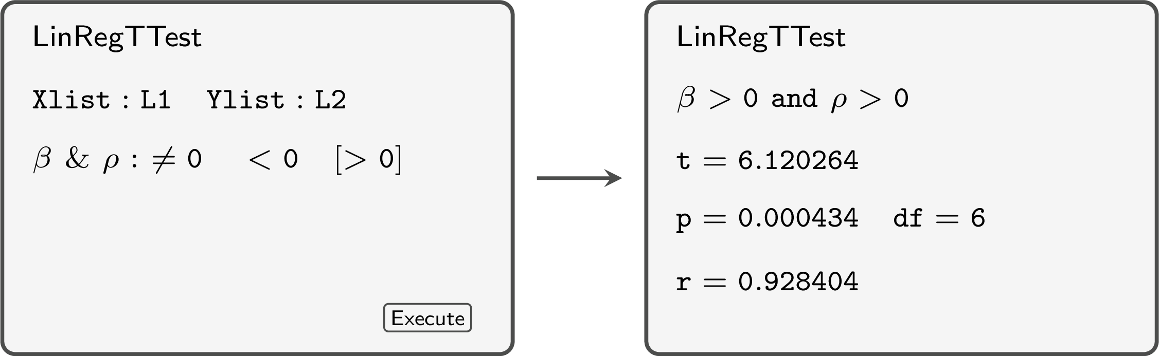
Test: run the linear regression $t$-test of the calculator (LinRegTTest), with the direction of $H_1$ (“$\beta$ and $\rho$”, where $\beta$ is the calculator's name for the gradient of the regression line, not the probability of a Type II error); it returns $t$, the p-value, the degrees of freedom $n - 2$ and $r$.
Decision and conclusion: reject $H_0$ if $p\text{-value} \leq \alpha$, and conclude in context about a linear correlation in the population — never about causation.

The mock-up shows the test of the next example.

Example

The table gives, for $8$ pupils chosen at random, the number of hours $x$ spent revising and the score $y$ obtained in a test.

$x$ (h)	$2$	$4$	$5$	$6$	$8$	$9$	$11$	$12$
$y$	$48$	$55$	$51$	$60$	$63$	$58$	$70$	$72$

Assuming a bivariate normal population, test at the $1\pourcent$ significance level whether there is a positive correlation between revision time and score.

Answer

Let $\rho$ be the correlation coefficient between revision time and score for all the pupils.

$H_0 : \rho = 0$ and $H_1 : \rho > 0$.
Bivariate normal population: test of $\rho = 0$ at $\alpha = 0.01$, with $8 - 2 = 6$ degrees of freedom.
The calculator (LinRegTTest, $\rho > 0$) gives $r \approx 0.928$ and $p\text{-value} \approx 0.000434$. By the formula: $$\begin{aligned}[t] t &= r\sqrt{\frac{n - 2}{1 - r^2}} && \text{(statistic of the test of } \rho = 0\text{)} \\ &\approx 0.9284\sqrt{\frac{6}{1 - 0.9284^2}} \approx 6.12. \end{aligned}$$
$0.000434 \leq 0.01$: reject $H_0$.
At the $1\pourcent$ level, there is a positive linear correlation between revision time and score in the population. The test says nothing about causation: other factors, such as motivation, may drive both.

Skills to practice

Testing $\rho \equal 0$ with Technology

VII Going further

Skills to practice

Problems: Testing Hypotheses
Quiz

\(H_1\)	\(\mu > \mu_0\)	\(\mu < \mu_0\)	\(\mu \neq \mu_0\)
\(p\text{-value}\)	\(P(Z \geq z)\)	\(P(Z \leq z)\)	\(2\,P(Z \geq \|z\|)\)

\(H_1\)	\(\mu > \mu_0\)	\(\mu < \mu_0\)	\(\mu \neq \mu_0\)
critical region	\(z \geq z_\alpha\)	\(z \leq -z_\alpha\)	\(z \leq -z_{\alpha/2}\) or \(z \geq z_{\alpha/2}\)

\(\alpha\)	\(0.10\)	\(0.05\)	\(0.01\)
one-tailed \(z_\alpha\)	\(1.282\)	\(1.645\)	\(2.326\)
two-tailed \(z_{\alpha/2}\)	\(1.645\)	\(1.960\)	\(2.576\)

\(\mu > \mu_0\)	\(\mu < \mu_0\)	\(\mu \neq \mu_0\)
\(\bar{x} \geq \mu_0 + z_\alpha\,\sigma/\sqrt{n}\)	\(\bar{x} \leq \mu_0 - z_\alpha\,\sigma/\sqrt{n}\)	\(\bar{x} \leq \mu_0 - z_{\alpha/2}\,\sigma/\sqrt{n}\) or \(\bar{x} \geq \mu_0 + z_{\alpha/2}\,\sigma/\sqrt{n}\)

\(H_1\)	\(p > p_0\)	\(p < p_0\)
\(p\text{-value}\)	\(P(X \geq x)\)	\(P(X \leq x)\)
critical region	\(X \geq c\)	\(X \leq c\)
choice of \(c\)	smallest \(c\) with \(P(X \geq c) \leq \alpha\)	largest \(c\) with \(P(X \leq c) \leq \alpha\)

	\(H_0\) is True	\(H_0\) is False
Reject \(H_0\)	Type I Error	Correct Decision
Fail to Reject \(H_0\)	Correct Decision	Type II Error

\(k\)	\(31\)	\(32\)	\(33\)
\(P(X \leq k)\)	\(0.0155\)	\(0.0419\)	\(0.0995\)

Value of \(\|r\|\)	Strength of Correlation
\(\|r\| = 1\)	Perfect
\(0.9 \le \|r\| < 1\)	Very Strong
\(0.7 \le \|r\| < 0.9\)	Strong
\(0.5 \le \|r\| < 0.7\)	Moderate
\(0.3 \le \|r\| < 0.5\)	Weak
\(0 \le \|r\| < 0.3\)	Very Weak or None

\(x\) (h)	\(2\)	\(4\)	\(5\)	\(6\)	\(8\)	\(9\)	\(11\)	\(12\)
\(y\)	\(48\)	\(55\)	\(51\)	\(60\)	\(63\)	\(58\)	\(70\)	\(72\)