International Baccalaureate · DP 2: Applications and Interpretation HL
Differential Equations
I
Differential Equations and Their Solutions
I.1
Fundamentals of Differential Equations
Definition — Differential Equation
A differential equation is an equation that contains an unknown function and one or more of its derivatives. - The order of a differential equation is the order of the highest derivative it contains.
- A general solution is a family of functions that satisfies the equation, typically involving one or more arbitrary constants.
- An initial condition is a specified value of the function or its derivatives at a particular point.
- A particular solution is a specific solution. It can be obtained by using one or more initial conditions (one per arbitrary constant) to determine the values of the arbitrary constants in the general solution.
Definition — Solution of a Differential Equation
A solution of a differential equation on an interval \(I\) is any function, differentiable on \(I\) as many times as the equation requires, that satisfies the equality for every \(x\) in \(I\).The order of a differential equation is the order of the highest derivative of the unknown function appearing in it (\(1\) for \(y'\), \(2\) for the second derivative \(y''\)): \(y' = 2y - 6\) is a first-order equation, \(y'' - y = 0\) a second-order equation.
Solving a differential equation means finding all the solution functions that satisfy the equality.
Example
The function \(x \mapsto e^{-x}\) is a solution of the equation \(y'' - y = 0\) because, for \(y(x) = e^{-x}\), we have \(y'(x) = -e^{-x}\) and \(y''(x) = e^{-x}\). Thus, \(y''(x) - y(x) = e^{-x} - e^{-x} = 0\).
Definition — Understanding Notations
It is crucial to understand that in a differential equation, \(y\) is a function, not a fixed number. Depending on the context (Mathematics, Physics, or Engineering), we use different notations for the unknown function and its derivative: - Lagrange notation: Uses a "prime" symbol (\(y'\)). This is the most common shorthand in Math.
- Leibniz notation: Uses a differential ratio (\(\dfrac{\mathrm{d}y}{\mathrm{d}t}\) or \(\dfrac{\mathrm{d}y}{\mathrm{d}x}\)). This explicitly shows which variable we are differentiating with respect to (usually time \(t\) or position \(x\)).
- Functional notation: Explicitly writes \(y(t)\) or \(y(x)\) to remind us that the value depends on the variable.
Example
The following three equations represent exactly the same relationship where \(y\) is a function of time \(t\): - Shorthand style: \(2y' + 3y = t\)
- Functional style: \(2y'(t) + 3y(t) = t\)
- Differential style (Leibniz): \(2\dfrac{\mathrm{d}y}{\mathrm{d}t} + 3y(t) = t\)
Example
An apple is dropped from rest at a height of 10 meters. Its vertical position, \(y(t)\), is governed by the second-order differential equation: $$\frac{d^2 y}{\mathrm{d}t^2}=-g$$ where \(g\) is the constant of gravitational acceleration. 
- State the initial conditions for position \(y(0)\) and velocity \(y'(0)\).
- Verify that the general solution to this equation is \(y(t) = -\frac{1}{2}gt^2 + At + B\).
- Use the initial conditions to find the particular solution for the apple's motion.
- Initial Conditions:
- The initial height is 10 meters, so \(y(0)=10\).
- The apple is dropped “from rest,” so its initial velocity is zero. Thus, \(y'(0)=0\).
- Verifying the General Solution: We need to show that the second derivative of \(y(t) = -\frac{1}{2}gt^2 + At + B\) is equal to \(-g\).
- First derivative (velocity): \(y'(t) = \dfrac{d}{\mathrm{d}t}\left(-\frac{1}{2}gt^2 + At + B\right) = -gt + A\).
- Second derivative (acceleration): \(y''(t) = \dfrac{d}{\mathrm{d}t}(-gt + A) = -g\).
- Finding the Particular Solution: We apply the initial conditions to the general solution and its first derivative.
- Using \(y(0)=10\): $$ y(0) = -\frac{1}{2}g(0)^2 + A(0) + B \implies 10 = B $$
- Using \(y'(0)=0\): $$ y'(0) = -g(0) + A \implies 0 = A $$
Skills to practice
- Defining and Verifying Differential Equations
- Checking Solutions of Differential Equations
- Modeling with Differential Equations
I.2
Slope Fields
While algebraic techniques give us formulas for solutions, a geometric approach can give us a powerful intuition for how solutions behave. A differential equation of the form \(\dfrac{\mathrm{d}y}{\mathrm{d}x} = f(x, y)\) is a machine that gives us the slope of a solution curve at any point \((x,y)\) where the expression is defined.
A slope field (or direction field) is a graphical representation of this information. At each point on a grid, we draw a small line segment with the slope given by the differential equation. The resulting field of slopes acts like a set of “currents” in a river. Any particular solution to the differential equation is a curve that “flows” along these currents, always tangent to the slope markers it passes through. 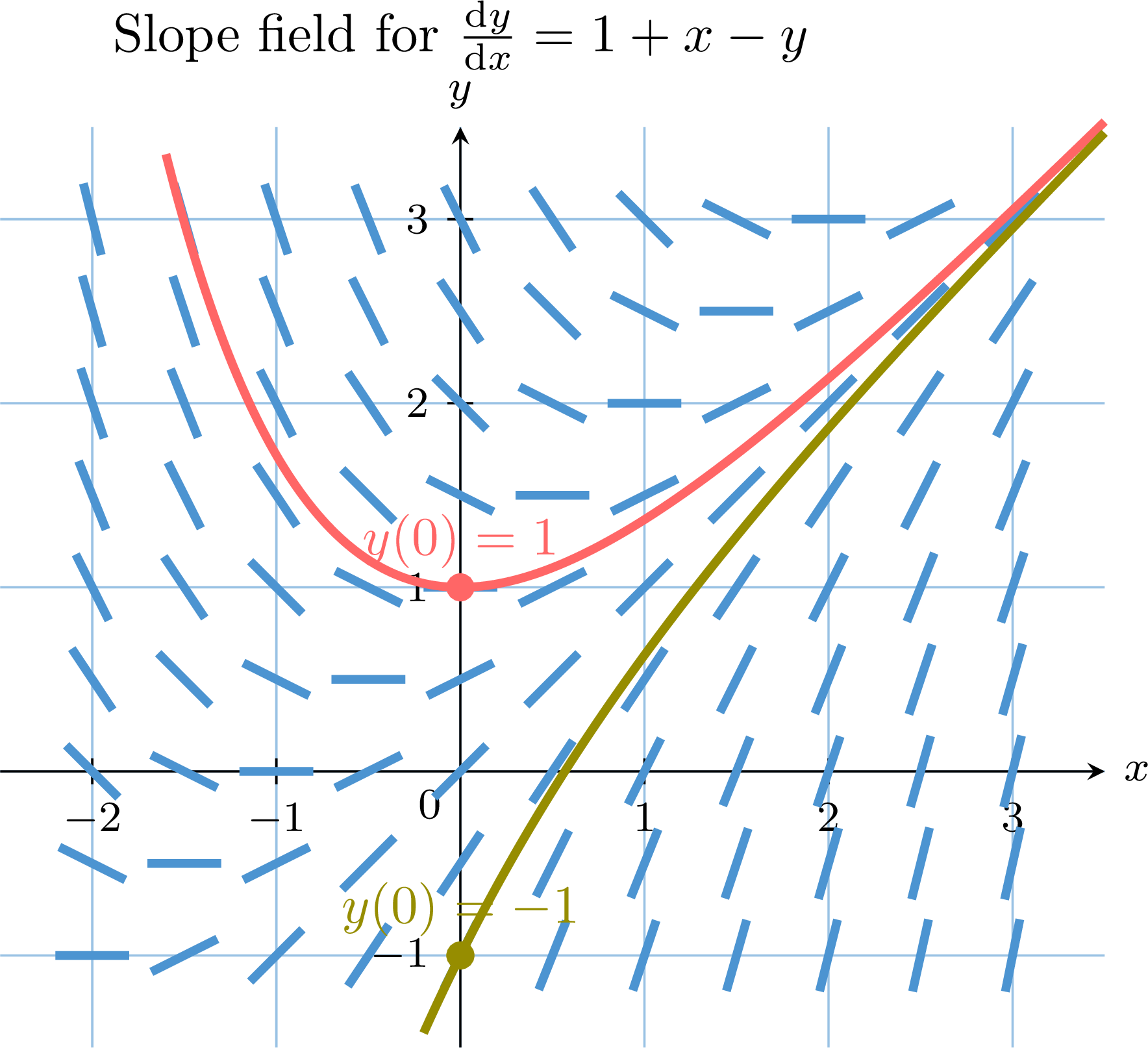
A slope field (or direction field) is a graphical representation of this information. At each point on a grid, we draw a small line segment with the slope given by the differential equation. The resulting field of slopes acts like a set of “currents” in a river. Any particular solution to the differential equation is a curve that “flows” along these currents, always tangent to the slope markers it passes through.
Method — Sketching a Slope Field
To sketch a slope field for \(\dfrac{\mathrm{d}y}{\mathrm{d}x} = f(x, y)\): - Choose grid points: Select a representative set of integer points \((x, y)\) in the desired viewing window.
- Calculate slopes: For each point, calculate the value of the slope \(m = f(x, y)\). Organize these values in a table.
- Sketch segments: At each grid point, draw a short line segment with the calculated slope.
Example
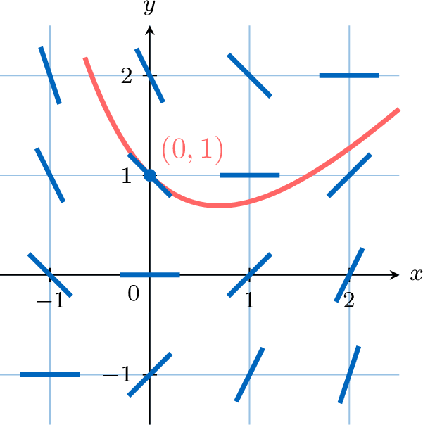
For the differential equation \(\dfrac{\mathrm{d}y}{\mathrm{d}x} = x-y\): - Sketch the slope field for integer coordinates where \(-1 \le x \le 2\) and \(-1 \le y \le 2\).
- On your sketch, draw the particular solution curve that passes through the point \((0,1)\).
- Sketching the field: We first calculate the slopes \(m=x-y\) at each integer point in the grid.
\(\begin{aligned} & x\\ y \end{aligned} \) -1 0 1 2 2 -3 -2 -1 0 1 -2 -1 0 1 0 -1 0 1 2 -1 0 1 2 3 - Drawing the solution curve: Starting at the initial point \((0,1)\), we follow the direction of the slope field. The curve will be tangent to the line segments as it passes through the field.
Skills to practice
- Reading a Slope Field
- Sketching Slope Fields
II
Exact Solutions
II.1
Solving by Direct Integration
Method — Solving for \(\frac{dy}{dx} \equal f(x)\)
When the derivative of a function depends only on \(x\), we can find the general solution by rearranging the equation and integrating directly. $$ \begin{aligned} \frac{\mathrm{d}y}{\mathrm{d}x} &= f(x)\\
\mathrm{d}y &= f(x)\, \mathrm{d}x \\
\int \mathrm{d}y &= \int f(x) \, \mathrm{d}x \\
y &= \int f(x) \, \mathrm{d}x + C \end{aligned} $$ Example
Find the general solution to \(\dfrac{\mathrm{d}y}{\mathrm{d}x} = 3x^2 \) and the particular solution with initial condition \(y(0)=4\).
We rearrange and integrate both sides: $$ \begin{aligned} \dfrac{\mathrm{d}y}{\mathrm{d}x} &= 3x^2 \\
\mathrm{d}y &= 3x^2 \, \mathrm{d}x \\
\int \mathrm{d}y &= \int 3x^2\, \mathrm{d}x \\
y & = x^3 + C \end{aligned} $$ This is the general solution. Now we use the initial condition \(y(0)=4\): $$ 4 = (0)^3 + C \implies C=4 $$ The particular solution is \(y = x^3 + 4\).
Skills to practice
- Solving by Direct Integration
- Finding Particular Solutions by Integration
II.2
Growth and Decay Models
When the Derivative Depends on the Function
In \(y' = f\), the derivative of the unknown function is given: for the usual functions, reading the table of derivatives backwards finds the function. In \(y' = ay\), the derivative depends on the unknown function itself — a quantity whose rate of change is proportional to its value, like the number of atoms in a radioactive sample. No table read backwards gives the answer; the exponential function does.
Proposition — Solutions of \(y' \equal ay\)
Let \(a\) be a real number.The solutions to the differential equation \(y' = ay\) are the functions defined on \(\mathbb{R}\) by: $$ \textcolor{colorprop}{y(x) = K e^{ax}} \quad \text{where } K \in \mathbb{R} \text{ is a constant.} $$
Every function of the form \(y(x) = K e^{ax}\) is clearly a solution since \(y'(x) = aKe^{ax} = ay(x)\).
To prove that all solutions are of this form, let \(y\) be any solution of \(y' = ay\). We look for \(y\) in the form:$$ y(x) = K(x) e^{ax} $$ where \(K\) is a function to be determined. Since \(y\) is differentiable, \(K(x) = y(x)e^{-ax}\) is also differentiable. Differentiating \(y\):$$ \begin{aligned}y'(x) &= K'(x)e^{ax} + K(x) \cdot (ae^{ax}) \\ y'(x) &= K'(x)e^{ax} + a \underbrace{K(x)e^{ax}}_{y(x)} \\ y'(x) &= K'(x)e^{ax} + ay(x) \\ y'(x) &= K'(x)e^{ax} + y'(x)\qquad (\text{as } y' = ay) \\ K'(x)e^{ax} &= 0\end{aligned} $$ As \(e^{ax} \neq 0\) for all \(x\), it follows that \(K'(x) = 0\).
This implies that \(K(x)\) is a constant \(K\). Thus, \(y(x) = Ke^{ax}\).
Example
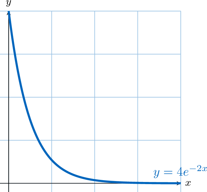
Solve the differential equation \(y' = -2y\) with the initial condition \(y(0) = 4\). - General solution: The equation is of the form \(y' = ay\) with \(a = -2\). The general solutions are the functions: $$ y(x) = K e^{-2x} \quad \text{where } K \in \mathbb{R} $$
- Particular solution: Using the initial condition \(y(0) = 4\): $$ K e^{-2(0)} = 4 \implies K \times 1 = 4 \implies K = 4 $$ The unique solution is \(y(x) = 4e^{-2x}\).
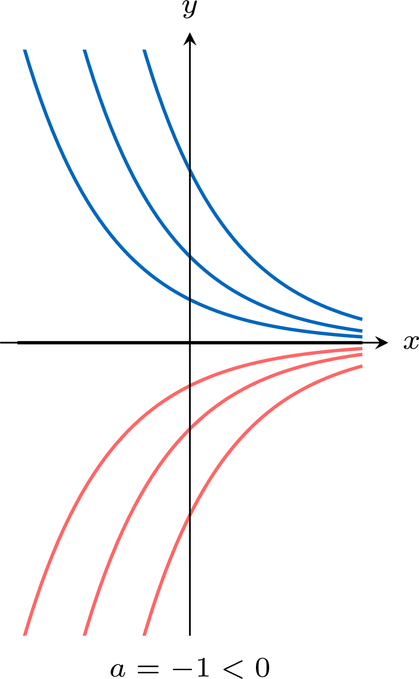
The solution curves \(y = Ke^{ax}\) form a family filling the plane. The sign of \(K\) decides the side of the \(x\)-axis (the curve \(K = 0\) is the axis, and no other curve ever crosses it); the sign of \(a\) decides the behaviour: for \(a > 0\) the curves move away from the axis, for \(a < 0\) they approach it. 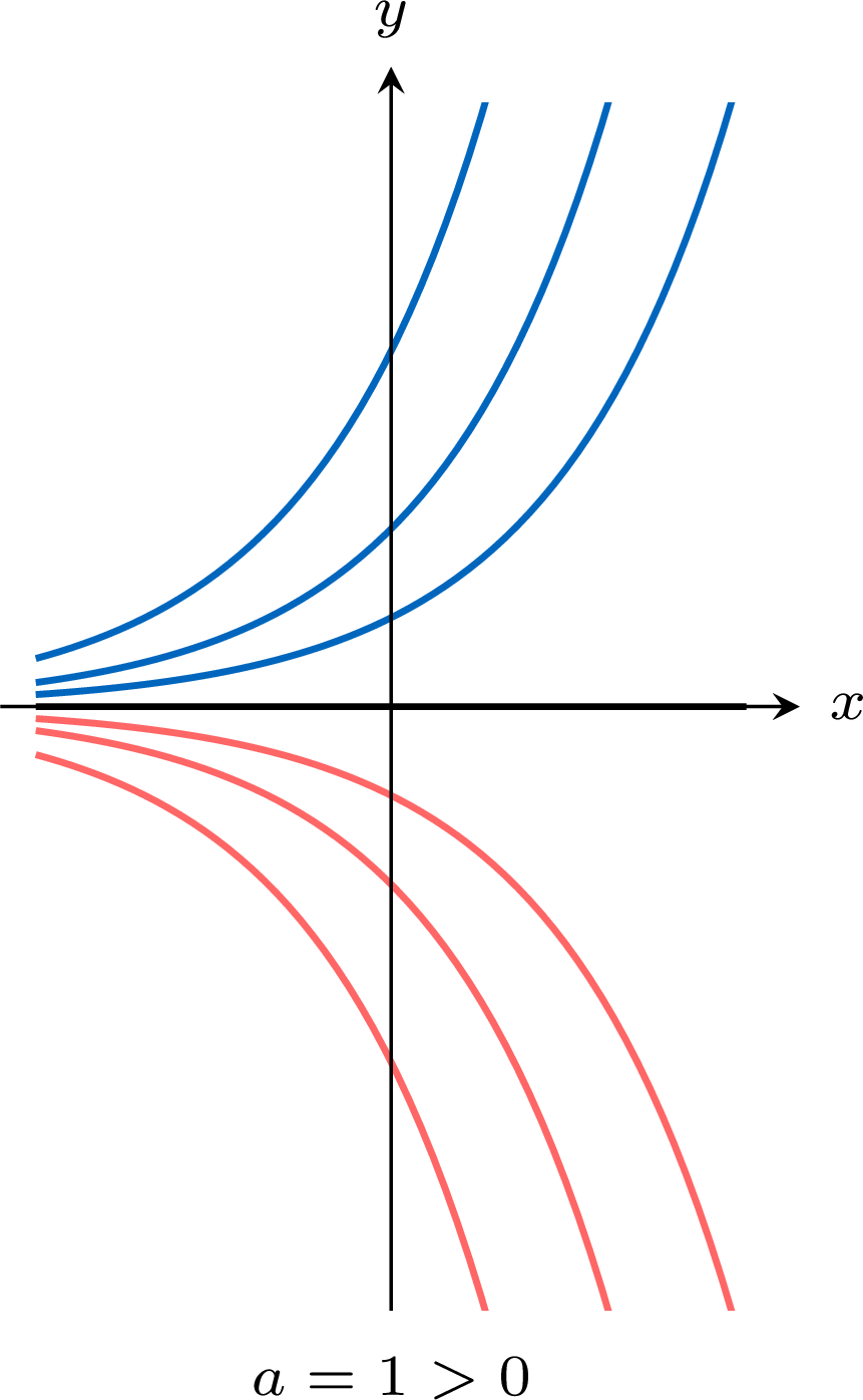 \(\qquad\)
\(\qquad\)
Discrete Model, Continuous Model
A quantity that grows by \(3\pourcent\) per year can be modelled in two ways.
The bridge between the two models is the tangent approximation: over a short time \(h\), \(y(t + h) \approx y(t) + h\,y'(t)\). For \(y' = ay\) with \(h = 1\), this gives \(y(t + 1) \approx (1 + a)\,y(t)\) when \(a\) is small (here \(a = 0.03\)): reading the continuous model once a year produces, approximately, a geometric sequence of ratio \(1 + a\); the exact ratio is \(e^{a}\), and \(1 + a\) is its tangent approximation at \(0\). The same step, repeated from an initial value, is the method studied in the last section of this chapter.
- Discrete model: the quantity is only looked at once a year. Its values \(u_0, u_1, u_2, \dots\) form a geometric sequence of ratio \(1.03\): \(u_{n+1} = 1.03\,u_n\), so \(u_n = 1.03^n\,u_0\).
- Continuous model: the quantity is a function \(y\) of the time \(t\), and at every instant its rate of change is proportional to its value, with rate \(0.03\) per year: \(y' = 0.03\,y\), so \(y(t) = y_0\,e^{0.03t}\).
The bridge between the two models is the tangent approximation: over a short time \(h\), \(y(t + h) \approx y(t) + h\,y'(t)\). For \(y' = ay\) with \(h = 1\), this gives \(y(t + 1) \approx (1 + a)\,y(t)\) when \(a\) is small (here \(a = 0.03\)): reading the continuous model once a year produces, approximately, a geometric sequence of ratio \(1 + a\); the exact ratio is \(e^{a}\), and \(1 + a\) is its tangent approximation at \(0\). The same step, repeated from an initial value, is the method studied in the last section of this chapter.
Example — Radioactive Decay: Discrete Model, Continuous Model
A radioactive substance loses \(1.2\pourcent\) of its nuclei every century. Let \(N_0\) be the number of nuclei at the start. - Discrete model. Let \(u_n\) be the number of nuclei after \(n\) centuries. Express \(u_n\) in terms of \(n\) and \(N_0\).
- Continuous model. Let \(N(t)\) be the number of nuclei after \(t\) centuries; at every instant, the nuclei disintegrate at a rate proportional to their number, and the instantaneous rate \(0.012\) is taken as an approximation of the loss of \(1.2\pourcent\) per century: \(N' = -0.012\,N\). Determine \(N(t)\) in terms of \(t\) and \(N_0\).
- Compare the two models after five centuries.
- In the continuous model, determine the half-life: the time after which half of the nuclei remain. In the discrete model, determine the first century at the end of which at most half of the nuclei remain.
- Losing \(1.2\pourcent\) means multiplying by \(1 - 0.012 = 0.988\) each century: \(u_{n+1} = 0.988\,u_n\), so \((u_n)\) is a geometric sequence of ratio \(0.988\) and first term \(u_0 = N_0\): $$ u_n = N_0 \times 0.988^{\,n}. $$
- The equation \(N' = -0.012\,N\) is of the form \(y' = ay\) with \(a = -0.012\): its solutions are the functions \(N(t) = Ke^{-0.012t}\), \(K \in \mathbb{R}\). The initial condition \(N(0) = N_0\) gives \(K = N_0\): $$ N(t) = N_0\,e^{-0.012t}. $$
- After five centuries: $$\begin{aligned} u_5 &= N_0 \times 0.988^{5} \approx 0.9414\,N_0, \\ N(5) &= N_0\,e^{-0.06} \approx 0.9418\,N_0. \end{aligned}$$ Both models keep about \(94\pourcent\) of the nuclei; they differ by less than \(0.05\pourcent\) of \(N_0\). The continuous model decays slightly more slowly, because \(e^{-0.012} \approx 0.98807 > 0.988\).
- In the continuous model, \(N(t) = \dfrac{N_0}{2}\) means \(e^{-0.012t} = \dfrac{1}{2}\), that is \(-0.012t = \ln \dfrac{1}{2} = -\ln 2\) (\(\ln\) is the inverse function of \(\exp\)), so $$ t = \frac{\ln 2}{0.012} \approx 57.8. $$ The half-life is about \(57.8\) centuries. It does not depend on \(N_0\): whatever the amount, it halves in the same time.
In the discrete model, the number of nuclei is only known at whole centuries: \(u_n \le \dfrac{N_0}{2}\) means \(0.988^{\,n} \le \dfrac{1}{2}\). Both sides are strictly positive and \(\ln\) is strictly increasing: $$\begin{aligned} 0.988^{\,n} \le \frac{1}{2} &\iff n \ln 0.988 \le \ln \frac{1}{2} &&\text{(\(\ln q^n = n \ln q\))} \\ &\iff n \ge \frac{\ln 0.5}{\ln 0.988} \approx 57.4 &&\text{(division by \(\ln 0.988 < 0\): direction reversed)}. \end{aligned}$$ So \(n = 58\): at the end of the \(58\)th century, for the first time, at most half of the nuclei remain (check: \(0.988^{57} \approx 0.503\), \(0.988^{58} \approx 0.497\)). The two models agree to within a century over more than five thousand years.
When the Rate Depends on a Gap
A bowl of soup at \(90\,^\circ\mathrm{C}\) is left in a room at \(18\,^\circ\mathrm{C}\). Its temperature \(T(t)\), in degrees Celsius after \(t\) minutes, falls all the faster as the gap with the room is large; a model is $$T'(t) = -0.2\,\bigl(T(t) - 18\bigr), \quad \text{that is} \quad T' = -0.2\,T + 3.6.$$ This equation is not of the form \(y' = ay\): the constant \(3.6\) is in the way. Two remarks point to its solutions.
- The equilibrium. A constant temperature \(T = c\) has \(T' = 0\), so \(0 = -0.2\,c + 3.6\) and \(c = 18\): at the room temperature, the soup no longer cools.
- The gap. The gap \(z = T - 18\) has the same derivative as \(T\), and \(z' = T' = -0.2\,(T - 18) = -0.2\,z\): the gap is a solution of \(y' = -0.2\,y\), an equation already solved.
Proposition — Solutions of \(y' \equal ay + b\)
Let \(a\) and \(b\) be two real numbers with \(a \neq 0\).The solutions to the differential equation \(y' = ay + b\) are the functions defined on \(\mathbb{R}\) by: $$ \textcolor{colorprop}{y(x) = K e^{ax} - \dfrac{b}{a}} \quad \text{where } K \in \mathbb{R} \text{ is a constant.} $$ The constant \(-\frac{b}{a}\) is itself a solution: it is the unique constant (particular) solution of the equation.
Let \(c = -\dfrac{b}{a}\). The constant function \(y = c\) has \(y' = 0\), and \(ac + b = -b + b = 0\): it is a solution. Now let \(y\) be any function differentiable on \(\mathbb{R}\), and set \(z = y - c\), so that \(y = z + c\) and \(y' = z'\). Then: $$\begin{aligned} y \text{ is a solution of } y' = ay + b &\iff z' = a(z + c) + b \\
&\iff z' = az + (ac + b) \\
&\iff z' = az &&\text{(since } ac + b = 0\text{)} \\
&\iff z = Ke^{ax} \text{ with } K \in \mathbb{R} &&\text{(solutions of } y' = ay\text{)}. \end{aligned}$$ So the solutions are exactly the functions \(y = Ke^{ax} + c = Ke^{ax} - \dfrac{b}{a}\): the solutions of \(y' = ay + b\) are obtained by adding the constant solution to the solutions of \(y' = ay\). This is the method: find the constant solution \(c\) by solving \(0 = ac + b\), then add the solutions \(Ke^{ax}\).
Example
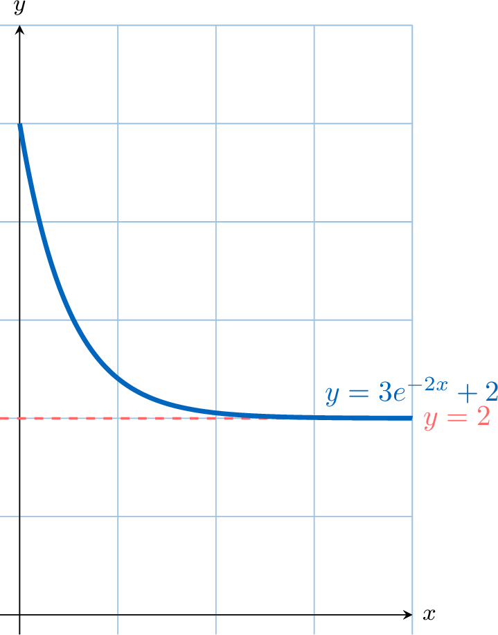
Solve the differential equation \(y' = -2y + 4\) with the initial condition \(y(0) = 5\). - Constant particular solution: we look for a constant solution \(y = c\): then \(y' = 0\), so \(0 = -2c + 4\), giving \(c = 2\).
General solution: by the proposition on the solutions of \(y' = ay + b\), the solutions are obtained by adding this constant to the solutions of \(y' = -2y\): $$ y(x) = K e^{-2x} + 2 \quad \text{where } K \in \mathbb{R} $$ - Particular solution: Using the initial condition \(y(0) = 5\): $$ K e^{-2(0)} + 2 = 5 \implies K + 2 = 5 \implies K = 3 $$ The unique solution is \(y(x) = 3e^{-2x} + 2\).
The equation \(y' = ay\) has a remarkable structure: if \(y_1\) and \(y_2\) are solutions of \(y' = ay\), then \(y_1 + y_2\) and \(\lambda y_1\) (for any real \(\lambda\)) are also solutions — substituting them into the equation shows it at once. This is special to it: for the equation \(y' = ay + b\) with a constant \(b \neq 0\), the sum of two solutions is not a solution.
Skills to practice
- Identifying Solutions of Growth and Decay Equations
- Solving with an Initial Condition
- Modelling and Solving with Differential Equations
II.3
Solving by Separation of Variables
A separable differential equation is one that can be expressed in the form \(\dfrac{\mathrm{d}y}{\mathrm{d}x} = g(x)h(y)\). These equations can be solved by algebraically separating the variables before integrating.
Method — Solving Separable Equations \(\frac{dy}{dx} \equal g(x)h(y)\)
This method applies when the equation can be rearranged so that all terms involving \(y\) are on one side and all terms involving \(x\) are on the other. - Separate: Rearrange the equation into the form \(\dfrac{1}{h(y)}\, \mathrm{d}y = g(x)\, \mathrm{d}x\).
- Integrate: Integrate both sides of the equation with respect to their respective variables: $$ \int \dfrac{1}{h(y)} \, \mathrm{d}y = \int g(x) \, \mathrm{d}x $$
- Solve for \(y\): If possible, solve the resulting equation for \(y\) to get an explicit solution.
Example
Solve \(\dfrac{\mathrm{d}y}{\mathrm{d}x} = -2xy^2\) with the initial condition \(y(1)=1\).
We rearrange and integrate both sides: $$ \begin{aligned} \dfrac{\mathrm{d}y}{\mathrm{d}x} &= -2xy^2 \\
\frac{1}{y^2} \, \mathrm{d}y &= -2x \, \mathrm{d}x \\
\int \frac{1}{y^2} \, \mathrm{d}y &= \int -2x \, \mathrm{d}x \\
\int y^{-2} \, \mathrm{d}y &= \int -2x \, \mathrm{d}x \\
-y^{-1} &= -x^2 + C \\
-\frac{1}{y} &= -x^2 + C \end{aligned} $$ This is the general solution in implicit form. Using the initial condition \(y(1)=1\): $$ -\dfrac{1}{1} = -(1)^2 + C \implies -1 = -1 + C \implies C = 0 $$ Substituting \(C=0\) gives the particular solution: $$ -\dfrac{1}{y} = -x^2 \implies y = \dfrac{1}{x^2} $$ This solution is defined on \((0, +\infty)\), the interval containing the initial point \(x = 1\). Note that the constant function \(y = 0\) (lost when dividing by \(y^2\)) is also a solution of the equation, but it does not satisfy the initial condition.
Skills to practice
- Solving Separable Equations
- Finding Particular Solutions by Separation
- Modelling with Separable Equations
II.4
Logistic Growth
Exponential growth \(\frac{\mathrm{d}P}{\mathrm{d}t} = kP\) assumes unlimited resources: the population grows without bound. Real populations live in environments that can only support a limited number of individuals. The logistic model refines the exponential model by making the growth rate shrink as the population approaches this limit.
Definition — The Logistic Equation
A population \(P(t)\) follows logistic growth when it satisfies$$ \frac{\mathrm{d}P}{\mathrm{d}t} = kP\left(1 - \frac{P}{A}\right), $$ where \(k > 0\) is the growth rate and \(A > 0\) is the carrying capacity — the largest population the environment can sustain. Proposition — Solution of the Logistic Equation
For an initial population \(P(0) = P_0\) with \(0 < P_0 < A\), the solution of the logistic equation is$$ P(t) = \frac{A}{1 + Ce^{-kt}}, \qquad C = \frac{A - P_0}{P_0}. $$ Moreover: - \(P(t) \to A\) as \(t \to \infty\): the population approaches the carrying capacity.
- The growth rate \(\frac{\mathrm{d}P}{\mathrm{d}t}\), viewed as a function of \(P\), is greatest at \(P = \frac{A}{2}\).
The equation is separable. For \(0 < P < A\), writing \(\frac{\mathrm{d}P}{\mathrm{d}t} = \frac{k}{A}P(A-P)\) and using the partial-fraction identity$$ \frac{A}{P(A-P)} = \frac{1}{P} + \frac{1}{A-P}, $$ we separate and integrate:$$\begin{aligned}\int \left(\frac{1}{P} + \frac{1}{A-P}\right) \mathrm{d}P &= \int k \, \mathrm{d}t \\
\ln P - \ln(A-P) &= kt + c \\
\frac{P}{A-P} &= Be^{kt} &&\text{(with } B = e^{c})\end{aligned}$$ Solving for \(P\) gives \(P = \dfrac{ABe^{kt}}{1 + Be^{kt}} = \dfrac{A}{1 + \frac{1}{B}e^{-kt}}\), so \(P(t) = \dfrac{A}{1 + Ce^{-kt}}\) with \(C = \frac{1}{B}\). The initial condition gives \(\frac{P_0}{A - P_0} = B\), hence \(C = \frac{A - P_0}{P_0}\).
As \(t \to \infty\), \(e^{-kt} \to 0\), so \(P(t) \to A\). Finally, \(\frac{\mathrm{d}P}{\mathrm{d}t} = kP - \frac{k}{A}P^2\) is a quadratic in \(P\) opening downwards, whose maximum is at \(P = \frac{A}{2}\).
As \(t \to \infty\), \(e^{-kt} \to 0\), so \(P(t) \to A\). Finally, \(\frac{\mathrm{d}P}{\mathrm{d}t} = kP - \frac{k}{A}P^2\) is a quadratic in \(P\) opening downwards, whose maximum is at \(P = \frac{A}{2}\).
Example
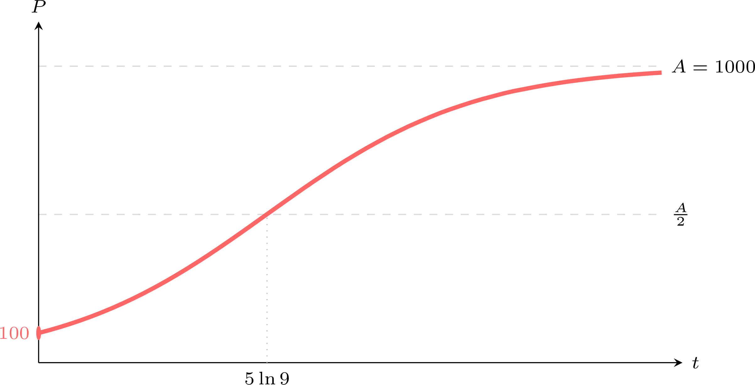
An island can sustain at most \(1000\) rabbits. The rabbit population, with \(t\) in years, follows the logistic equation$$ \frac{\mathrm{d}P}{\mathrm{d}t} = 0.2P\left(1 - \frac{P}{1000}\right), \qquad P(0) = 100. $$ - Find \(P(t)\).
- What is the limiting population?
- After how long does the population reach \(500\) rabbits, and why is the growth fastest at that moment?
- Here \(k = 0.2\), \(A = 1000\) and \(P_0 = 100\), so$$ C = \frac{A - P_0}{P_0} = \frac{1000 - 100}{100} = 9 \qquad\text{and}\qquad P(t) = \frac{1000}{1 + 9e^{-0.2t}}. $$
- As \(t \to \infty\), \(e^{-0.2t} \to 0\), so \(P(t) \to 1000\): the limiting population is the carrying capacity, \(1000\) rabbits.
- We solve \(P(t) = 500\):$$\begin{aligned}\frac{1000}{1 + 9e^{-0.2t}} &= 500 \\ 1 + 9e^{-0.2t} &= 2 \\ e^{-0.2t} &= \frac{1}{9} \\ t &= \frac{\ln 9}{0.2} = 5\ln 9 \approx 11.0 \text{ years.}\end{aligned}$$ The growth is fastest there because \(500 = \frac{A}{2}\), where the rate \(\frac{\mathrm{d}P}{\mathrm{d}t} = kP\left(1-\frac{P}{A}\right)\) reaches its maximum.
Skills to practice
- Computing with a Logistic Model
- Solving and Interpreting Logistic Models
III
Approximate Solutions
III.1
Approximating Solutions with Euler's Method
When a differential equation cannot be solved analytically, we can approximate its solution using numerical methods. Euler's method is the simplest of these, using linear approximation to step along the solution curve.
The method begins with an initial condition \((x_0, y_0)\) and proceeds in steps. Let's define a small, constant step size, \(h\). The \(x\)-coordinate of each subsequent point is found by adding this step size: \(x_{n+1} = x_n + h\).
The core of the method is to approximate the derivative \(\dfrac{\mathrm{d}y}{\mathrm{d}x}\) using the gradient of the line segment connecting two consecutive points, \((x_n, y_n)\) and \((x_{n+1}, y_{n+1})\): $$ \dfrac{\mathrm{d}y}{\mathrm{d}x} \text{ at } (x_n, y_n) \approx \dfrac{y_{n+1} - y_n}{x_{n+1} - x_n} = \dfrac{y_{n+1} - y_n}{h}. $$ Since the differential equation gives us the exact value of the derivative, \(\dfrac{\mathrm{d}y}{\mathrm{d}x} = f(x_n, y_n)\), we can set these equal: $$ \dfrac{y_{n+1} - y_n}{h}\approx f(x_n, y_n). $$ Rearranging this formula to find the next \(y\)-value, \(y_{n+1}\), gives the iterative step: $$ y_{n+1} \approx y_n + h \cdot f(x_n, y_n). $$ The collection of line segments created by this iterative procedure forms a polygonal approximation to the true solution curve. 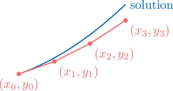
The method begins with an initial condition \((x_0, y_0)\) and proceeds in steps. Let's define a small, constant step size, \(h\). The \(x\)-coordinate of each subsequent point is found by adding this step size: \(x_{n+1} = x_n + h\).
The core of the method is to approximate the derivative \(\dfrac{\mathrm{d}y}{\mathrm{d}x}\) using the gradient of the line segment connecting two consecutive points, \((x_n, y_n)\) and \((x_{n+1}, y_{n+1})\): $$ \dfrac{\mathrm{d}y}{\mathrm{d}x} \text{ at } (x_n, y_n) \approx \dfrac{y_{n+1} - y_n}{x_{n+1} - x_n} = \dfrac{y_{n+1} - y_n}{h}. $$ Since the differential equation gives us the exact value of the derivative, \(\dfrac{\mathrm{d}y}{\mathrm{d}x} = f(x_n, y_n)\), we can set these equal: $$ \dfrac{y_{n+1} - y_n}{h}\approx f(x_n, y_n). $$ Rearranging this formula to find the next \(y\)-value, \(y_{n+1}\), gives the iterative step: $$ y_{n+1} \approx y_n + h \cdot f(x_n, y_n). $$ The collection of line segments created by this iterative procedure forms a polygonal approximation to the true solution curve.
Method — Euler's Method
To approximate the solution to \(\dfrac{\mathrm{d}y}{\mathrm{d}x} = f(x,y)\) with initial condition \((x_0, y_0)\) and a step size \(h\), the coordinates of the next point \((x_{n+1}, y_{n+1})\) are found from the previous point \((x_n, y_n)\) using the iterative formulas: $$ \begin{cases} x_{n+1} = x_n + h, \\
y_{n+1} = y_n + h \cdot f(x_n, y_n). \end{cases} $$ Proposition — Accuracy and Error
Euler's method is an approximation. The accuracy of this approximation depends on two main factors: - Step size (\(h\)): A smaller step size \(h\) generally leads to a more accurate approximation. As \(h \to 0\), the polygonal path of the approximation gets closer to the true solution curve. However, this comes at the cost of requiring more computational steps.
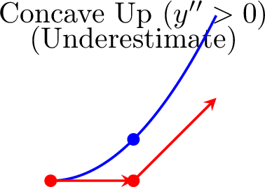
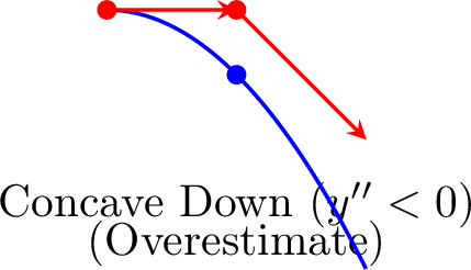
- Concavity of the solution curve: Each step follows the tangent line at its starting point, so the concavity of the solution curve through that point decides the direction of the error of the step. When the solutions keep a fixed concavity on the interval considered and the step \(h\) is small enough, the accumulated error keeps this direction, and the concavity determines whether the approximation is an overestimate or an underestimate.
- If the curve is concave up (\(\frac{d^2y}{\mathrm{d}x^2} > 0\)), the tangent line at the start of each step lies below the curve. With a small enough step, Euler's method produces an underestimate.
- If the curve is concave down (\(\frac{d^2y}{\mathrm{d}x^2} < 0\)), the tangent line lies above the curve: with a small enough step, the result is an overestimate.
- If the curve is concave up (\(\frac{d^2y}{\mathrm{d}x^2} > 0\)), the tangent line at the start of each step lies below the curve. With a small enough step, Euler's method produces an underestimate.
Example
Consider the differential equation \(\dfrac{\mathrm{d}y}{\mathrm{d}x} = -2xy\) with the initial condition \(y(0)=1\). - Use Euler's method with a step size of \(h=0.1\) to find an approximate value for \(y(0.2)\).
- By solving the differential equation, show that the particular solution is \(y(x) = e^{-x^2}\).
- Calculate the percentage error in your approximation from part 1.
- By considering the sign of \(\dfrac{d^2y}{\mathrm{d}x^2}\) in the interval \(0 \le x \le 0.2\), explain whether your approximation in part 1 is an overestimate or an underestimate of the true value.
- We start at \((x_0, y_0)=(0,1)\) with \(h=0.1\) and \(f(x,y)=-2xy\).
- Step 1: \(y_1 = y_0 + h \cdot (-2x_0y_0) = 1 + 0.1(-2\cdot 0 \cdot 1) = 1\). So, \(y(0.1) \approx 1\).
- Step 2: \(y_2 = y_1 + h \cdot (-2x_1y_1) = 1 + 0.1(-2\cdot 0.1 \cdot 1) = 1 - 0.02 = 0.98\).
- We solve by separating variables: $$ \frac{\mathrm{d}y}{\mathrm{d}x} = -2xy \implies \int \frac{1}{y} \, \mathrm{d}y = \int -2x \, \mathrm{d}x. $$ Thus $$ \ln|y| = -x^2 + C. $$ Using the initial condition \(y(0)=1\): $$ \ln|1| = -0^2 + C \implies C=0. $$ So, \(\ln y = -x^2\) (since \(y(0)=1>0\)), which gives the particular solution \(y(x) = e^{-x^2}\).
- The exact value is \(y_{\text{exact}} = e^{-(0.2)^2} = e^{-0.04} \approx 0.960789\ldots\) The approximate value is \(y_{\text{approx}} = 0.98\). The percentage error is $$ \text{Error} = \left|\frac{0.960789\ldots - 0.98}{0.960789\ldots}\right| \times 100\pourcent \approx 2.00\pourcent. $$
- To determine the nature of the error, we check the concavity by finding the second derivative: $$ \begin{aligned} \frac{d^2y}{\mathrm{d}x^2} &= \frac{d}{\mathrm{d}x}(-2xy) \\ &= -2\left(1 \cdot y + x \cdot \frac{\mathrm{d}y}{\mathrm{d}x}\right) \\ &= -2\bigl(y + x(-2xy)\bigr) \\ &= -2y(1-2x^2). \end{aligned} $$ At the start of the approximation, for \(x\) in \([0, 0.2]\), \(x^2\) is small, so \((1-2x^2)\) is positive. Since \(y\) is also positive in this region, the sign of the second derivative is $$ \frac{d^2y}{\mathrm{d}x^2} = (\text{negative})\times(\text{positive})\times(\text{positive}) < 0. $$ Since the second derivative is negative, the solution curve is concave down. Each step of Euler's method follows a tangent line, which lies above a concave down curve, so each step lands above the solution curve through its starting point. The step \(h = 0.1\) is small, so by the Proposition « Accuracy and Error » the errors keep this direction: the approximation is an overestimate (indeed \(0.98 > 0.9608\)).
Method — Euler's Method with Technology
Euler's method repeats the same two updates. A smaller step \(h\) generally gives a better approximation but needs more steps, and each step starts from the full value produced by the previous one. A spreadsheet or a graphing calculator performs the repetition and keeps every digit. - Set up the scheme on paper: the starting point \((x_0, y_0)\), the step \(h\), the number of steps \(n = \dfrac{b - x_0}{h}\) needed to reach \(x = b\) (\(h\) is chosen so that \(n\) is a whole number), and the formulas \(x_{k+1} = x_k + h\), \(y_{k+1} = y_k + h \cdot f(x_k, y_k)\).
- With a spreadsheet: one row per step. The first row holds \(k = 0\), \(x_0\) and \(y_0\). In the next row, \(x\) is the previous \(x\) plus \(h\), and \(y\) is the previous \(y\) plus \(h\) times \(f\) evaluated with the previous \(x\) and \(y\). These two formulas are filled down until \(x = b\).
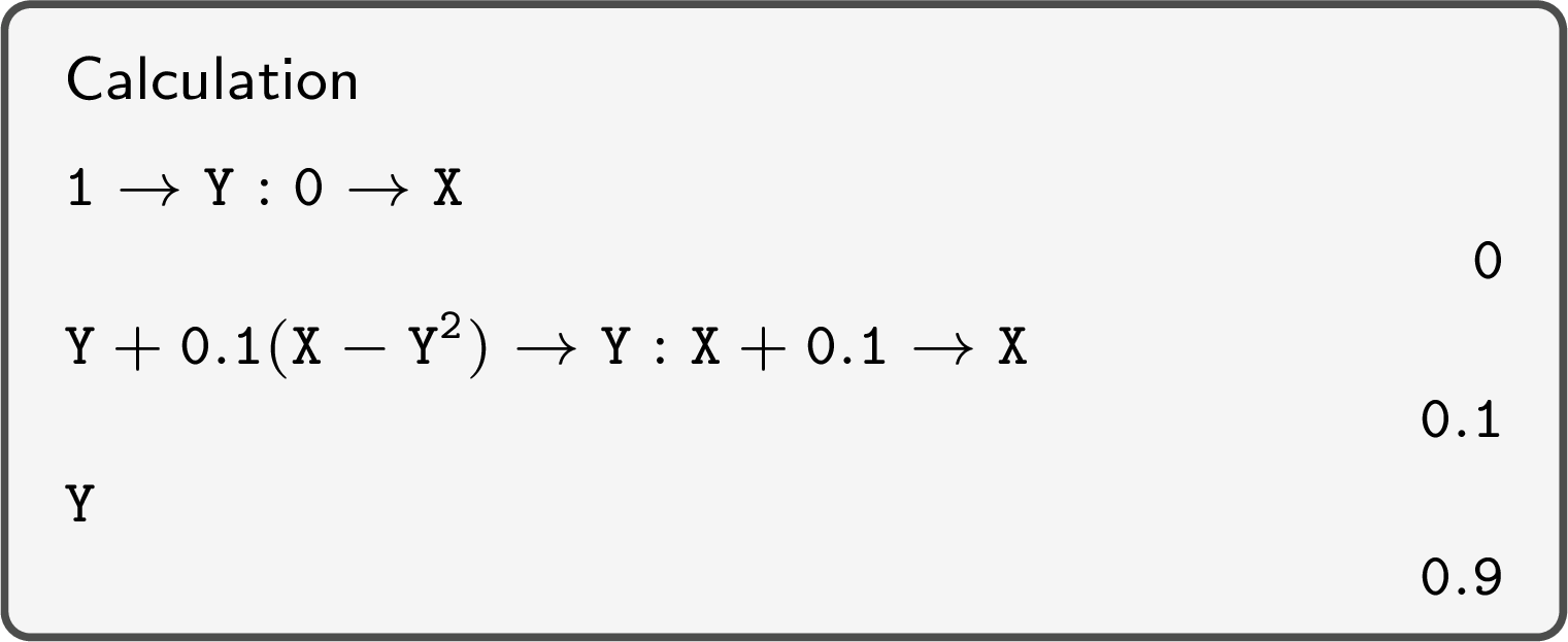
- With a graphing calculator: store \(x_0\) in \(X\) and \(y_0\) in \(Y\), then type the double command \(Y + h \cdot f(X, Y) \to Y : X + h \to X\). Each press of the execution key performs one step and displays the new value of \(X\). The value of \(Y\) is updated first, while \(X\) still holds the previous value.
- Report the last value of \(y\) to the accuracy asked, rounding only at the end. Written work shows the formulas and the first rows of the table, then the final value.
| A | B | C | |
| 1 | \(k\) | \(x\) | \(y\) |
| 2 | 0 | 0 | 1 |
| 3 | =A2+1 | =B2+0.1 | =C2+0.1*(B2-C2\^{}2) |
| 4 | 2 | 0.2 | 0.829 |
| \(\vdots\) | \(\vdots\) | \(\vdots\) | \(\vdots\) |
| 12 | 10 | 1 | 0.8053535 |
Example
The differential equation \(\dfrac{\mathrm{d}y}{\mathrm{d}x} = x - y^2\), with \(y(0) = 1\), cannot be solved by the methods of this chapter. - Use Euler's method with \(h = 0.1\) to estimate \(y(1)\), writing the first two steps and the number of steps.
- Use Euler's method with \(h = 0.05\) to estimate \(y(1)\).
- Explain which estimate is the more reliable.
- Here \(f(x, y) = x - y^2\), \(x_0 = 0\), \(y_0 = 1\), and \(n = \dfrac{1 - 0}{0.1} = 10\) steps reach \(x = 1\). The first two steps are $$\begin{aligned}[t] y_1 &= y_0 + h\,(x_0 - y_0^2) = 1 + 0.1\,(0 - 1) = 0.9, \\
y_2 &= y_1 + h\,(x_1 - y_1^2) = 0.9 + 0.1\,(0.1 - 0.81) = 0.829. \end{aligned}$$ The spreadsheet (or the calculator) continues to \(k = 10\):
\(k\) \(0\) \(1\) \(2\) \(3\) \(\cdots\) \(10\) \(x_k\) \(0\) \(0.1\) \(0.2\) \(0.3\) \(\cdots\) \(1\) \(y_k\) \(1\) \(0.9\) \(0.829\) \(0.780276\) \(\cdots\) \(0.805354\) - With \(h = 0.05\), \(n = \dfrac{1}{0.05} = 20\) steps: the same formulas, with \(0.05\) in place of \(0.1\), give \(y(1) \approx 0.8198\).
- By the Proposition « Accuracy and Error », a smaller step \(h\) generally gives a more accurate approximation: the estimate \(0.8198\), with \(h = 0.05\), is the more reliable. The two estimates differ by about \(0.014\): they do not agree to two decimal places, so the estimate with \(h = 0.1\) cannot be trusted to that accuracy.
Skills to practice
- Applying Euler's Method
- Applying Euler's Method with Technology
- Comparing Numerical and Analytical Solutions
IV
Going further
Skills to practice
- Solving Problems
- Quiz
Jump to section