International Baccalaureate · DP 2: Applications and Interpretation HL

Integration

⌚ ~186 min ▢ 21 blocks ✓ 94 exercises ➣ Prerequisites : Rules of Differentiation

I The Definite Integral as an Area

I.1 Approximating Area with Rectangles

The measurement of area has been fundamental to science and society since antiquity. In ancient Egypt, surveyors used knotted ropes to construct right angles, allowing them to measure and restore the boundaries of rectangular fields washed away by the annual floods of the Nile. While finding the area of shapes with straight sides is straightforward, calculus provides a revolutionary tool for finding the area of regions bounded by curves.

The aim is a method to find the exact area, $\mathcal{A}$, of the region bounded by the graph of a non-negative function $y=f(x)$, the x-axis, and the vertical lines $x=a$ and $x=b$. This area is denoted by the definite integral: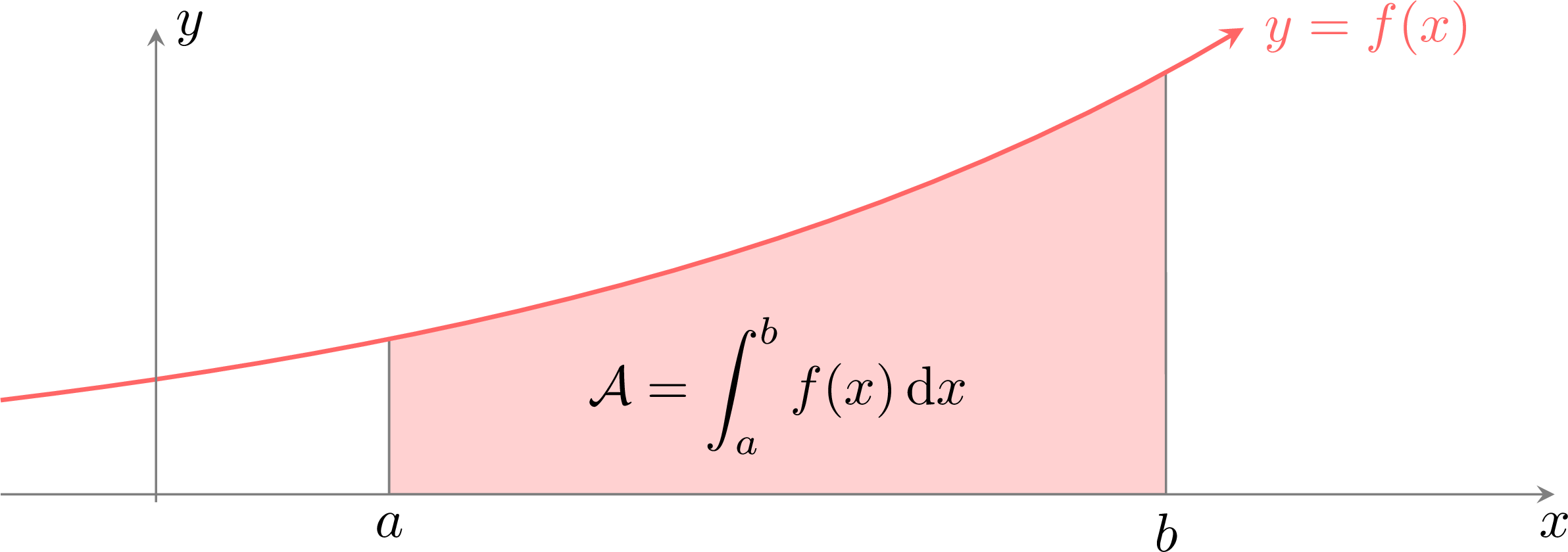

Report an error

Method — Approximating Area with Riemann Sums

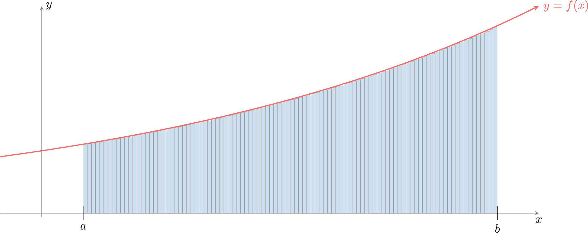
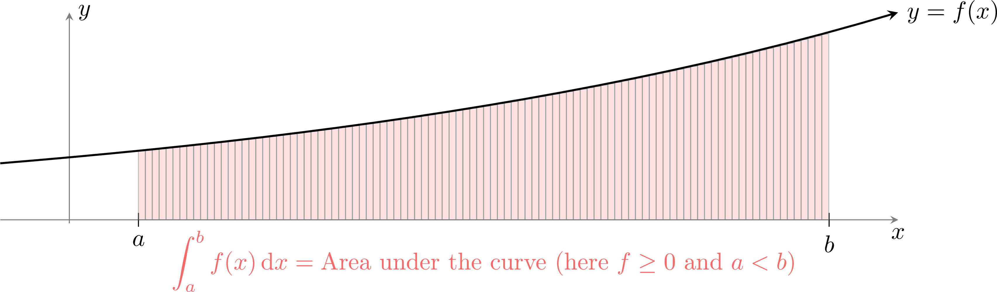
We aim to measure the shaded area, denoted $\displaystyle\int_a^b f(x)\,\mathrm{d}x$, under the curve of a continuous non-negative function $y=f(x)$.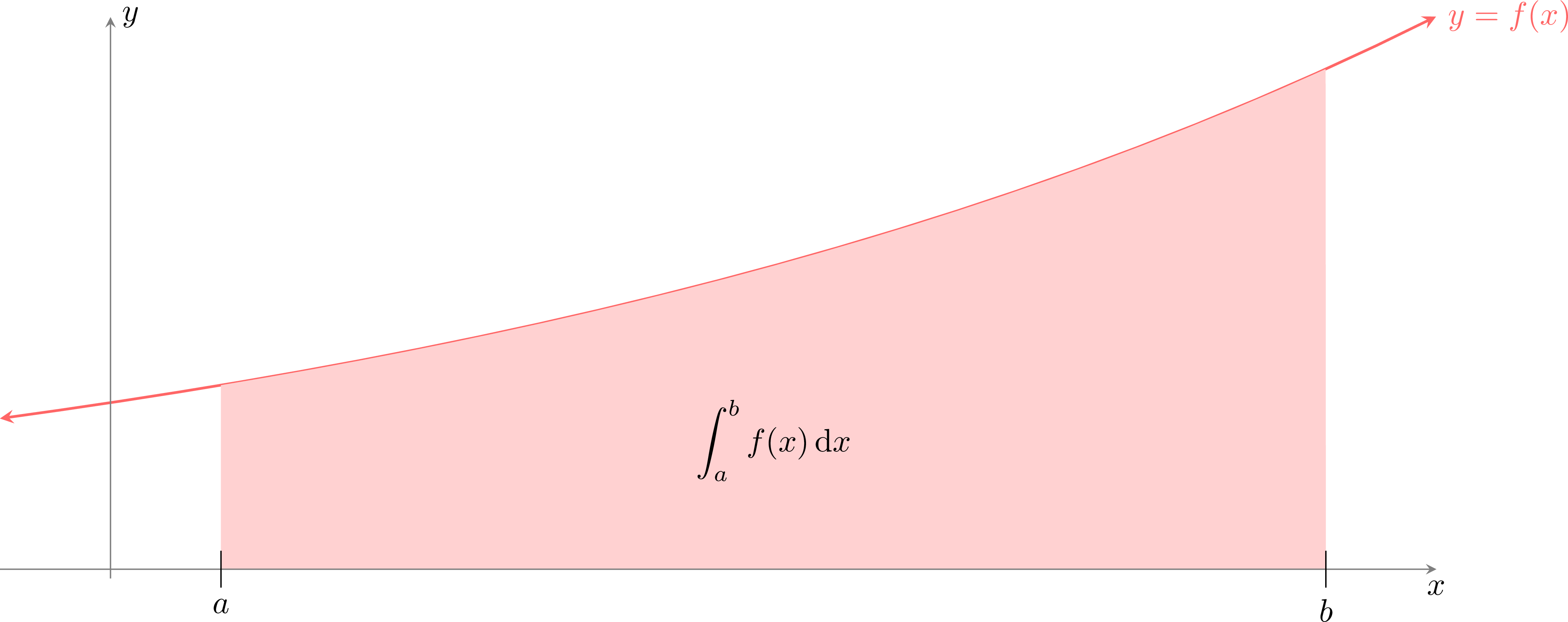

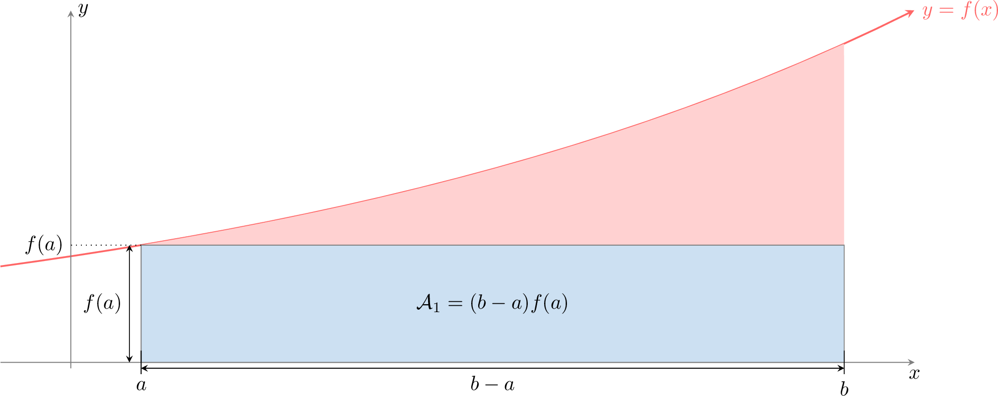
The key idea, developed by Bernhard Riemann, is to approximate this area by a sum of thin rectangles, known as a Riemann sum.

Approximation with 1 rectangle: We can make a first, rough approximation by filling the area with a single rectangle of width $(b-a)$ and height $f(a)$ (the value of the function at the left endpoint). The area is approximated by: $$\displaystyle\int_a^b f(x)\,\mathrm{d}x \approx (b-a)f(a)$$ For an increasing function, like the one shown, this is an underestimate.
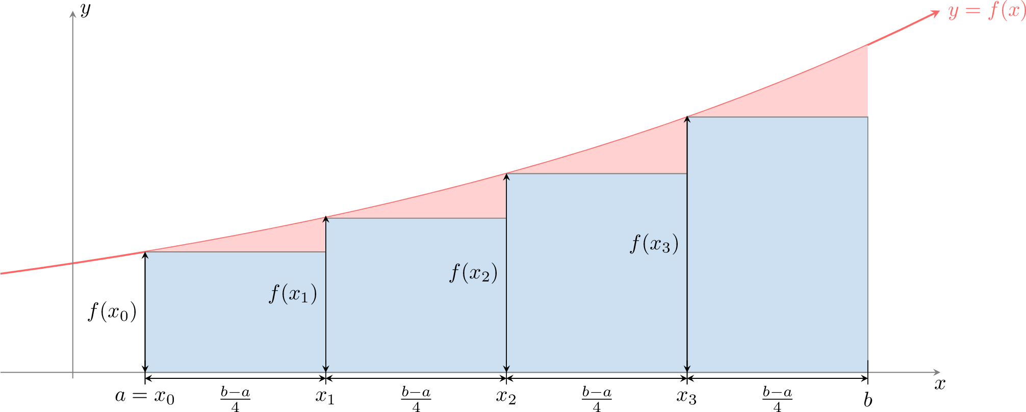
Approximation with 4 rectangles: To improve the approximation, we divide the interval $[a,b]$ into 4 equal subintervals, each of width $\frac{b-a}{4}$. We construct a rectangle on each subinterval, using the function's value at the left endpoint for the height. The total area of these four rectangles gives a much better approximation here, for the increasing function shown: $$\begin{aligned}[t]\displaystyle\int_a^b f(x)\,\mathrm{d}x &\approx \frac{b-a}{4}f(x_0)+\frac{b-a}{4}f(x_1)+\frac{b-a}{4}f(x_2)+\frac{b-a}{4}f(x_3) \\ &\approx \frac{b-a}{4} \left[f(x_0)+f(x_1)+f(x_2)+f(x_3)\right]\end{aligned}$$
Approximation with $n$ rectangles: We can generalise this by dividing the interval into $n$ equal subintervals, each of width $\Delta x = \frac{b-a}{n}$. Let $x_i=a+i\Delta x$ for $i=0,1,\dots,n-1$. The sum of the areas of the $n$ rectangles is: $$ S_n = \sum_{i=0}^{n-1} f(x_i) \Delta x. $$ As we increase the number of rectangles ($n \to \infty$), the width of each rectangle becomes infinitesimally small, and the sum of their areas becomes a perfect match for the area under the curve: $$\displaystyle\int_a^b f(x)\,\mathrm{d}x = \lim_{n\to\infty} S_n.$$

Skills to practice

Approximating Area with Rectangles

I.2 Definition of the Definite Integral

Definition — Definite Integral

The definite integral of a continuous function $f$ from $a$ to $b$ is the limit of the Riemann sum as the number of subintervals approaches infinity. It is denoted by: $$ \int_a^b f(x)\,\mathrm{d}x = \lim_{n \to \infty} \sum_{i=0}^{n-1} f(x_i) \Delta x $$ where the interval $[a,b]$ is divided into $n$ subintervals of equal width $\Delta x = \dfrac{b-a}{n}$ and $x_i = a + i\Delta x$.

$a$ and $b$ are the limits of integration.
$f(x)$ is the integrand.

This notation, introduced by Leibniz, captures the idea of summing ($ \int $ is an elongated 'S' for summa) the areas of infinitely many rectangles of height $f(x)$ and infinitesimal width $\mathrm{d}x$.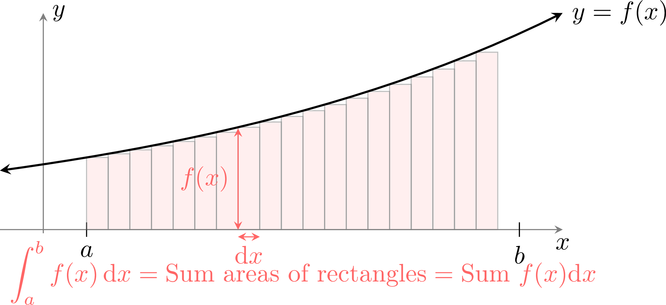

Report an error

Definition — Signed Area

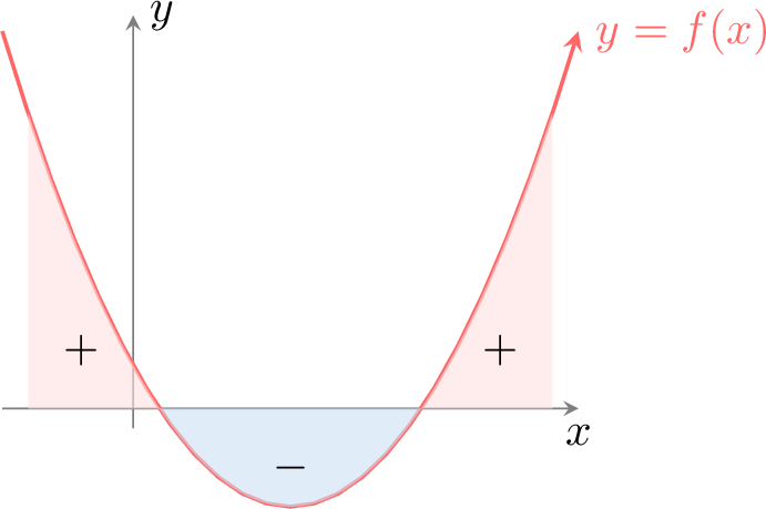
The definite integral calculates the signed area.

Area above the x-axis is counted as positive.
Area below the x-axis is counted as negative.

The integral is the sum of these signed areas.

Example

Determine the integral $\displaystyle\int_{-1}^{2} 1\,\mathrm{d}x$ by interpreting it as an area.

Answer

The integral represents the area under the constant function $f(x)=1$ from $x=-1$ to $x=2$. This forms a rectangle with width $2 - (-1) = 3$ and height $1$.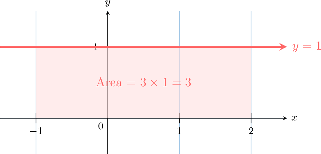

Therefore, $\displaystyle\int_{-1}^{2}1\,\mathrm{d}x= 3.$

Skills to practice

Identifying the Integral That Gives an Area
Reading the Sign of an Integral
Evaluating Integrals with Area Formulas

I.3 Properties of the Definite Integral

Proposition — Properties of Integration

Let $f$ and $g$ be continuous on an interval $I$, $a$, $b$, $c$ three real numbers in $I$, and $k$ a constant.

Zero-Width Interval: $$\displaystyle\int_a^a f(x) \;\mathrm{d}x= 0.$$
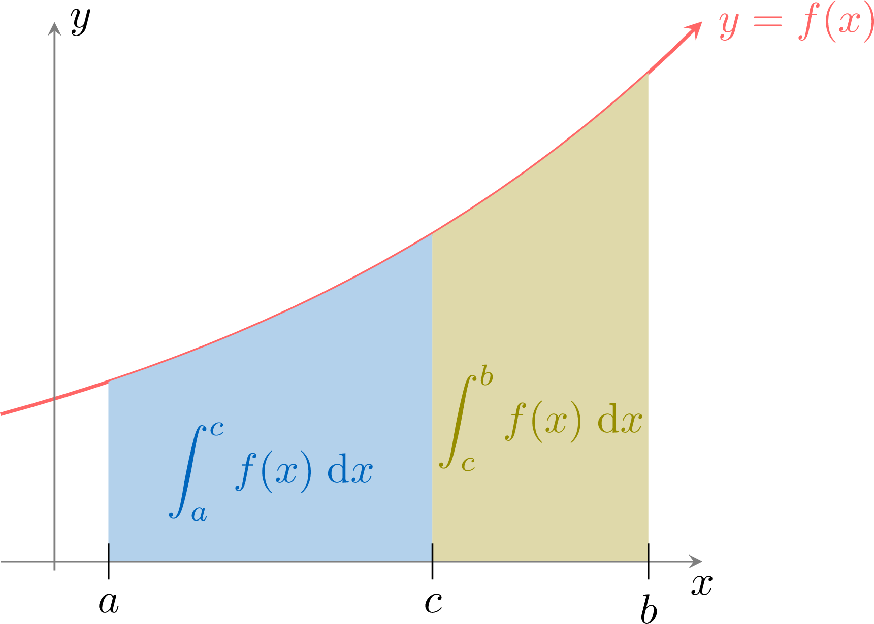
Additivity of Intervals: For any $c$ between $a$ and $b$: $$\displaystyle\int_a^b f(x)\;\mathrm{d}x = \int_a^c f(x) \; \mathrm{d}x + \int_c^b f(x)\;\mathrm{d}x$$
Linearity: $$\displaystyle\int_a^b (f(x)+g(x)) \; \mathrm{d}x= \int_a^b f(x) \; \mathrm{d}x+ \int_a^b g(x) \; \mathrm{d}x$$ $$\displaystyle\int_a^b k f(x) \; \mathrm{d}x= k \int_a^b f(x) \; \mathrm{d}x.$$

Skills to practice

Applying the Properties of Integrals

II Antiderivatives and the Fundamental Theorem

II.1 Antiderivatives

So far, we have defined the definite integral as the limit of a sum—a geometric concept of area. Separately, differentiation is a process of finding rates of change. The Fundamental Theorem of Calculus provides a profound and powerful link between these two seemingly unrelated ideas: integration and differentiation are inverse processes of each other.

Report an error

Definition — Antiderivative

A function $F$ is an antiderivative of a function $f$ if $F'(x) = f(x)$. The process of finding an antiderivative is called antidifferentiation or indefinite integration.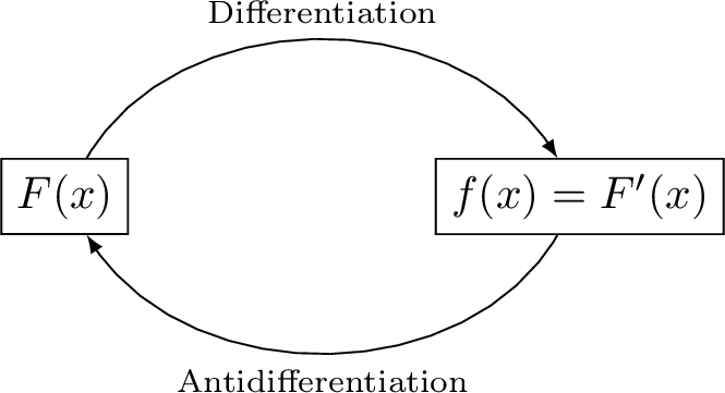

Since the derivative of a constant is zero, any function $f$ does not have a unique antiderivative. For example, if $F(x) = x^2$ is an antiderivative of $f(x)=2x$, then $G(x)=x^2+5$ is also an antiderivative, since $G'(x) = 2x+0 = 2x$. All antiderivatives of a function differ only by a constant.

Report an error

Proposition — Existence

Every continuous function on an interval $I$ admits antiderivatives on $I$ (a function continuous on an interval is a function whose graph can be drawn without lifting the pencil; all the functions studied here are continuous). This result is admitted; its proof uses integral calculus.

Proposition — General Form

If $F$ is an antiderivative of $f$ on an interval $I$, then any other antiderivative $G$ of $f$ on $I$ is defined by:$$ \textcolor{colorprop}{G(x) = F(x) + C} \quad \text{where } C \in \mathbb{R} \text{ is a constant.} $$

Proof

Let $F$ be a fixed antiderivative of $f$ on the interval $I$.

Analysis: Let $G$ be any antiderivative of $f$ on $I$.
By definition, $G'(x) = f(x)$ and $F'(x) = f(x)$.
Consider the function $H = G - F$. Its derivative is: $$ H'(x) = G'(x) - F'(x) = f(x) - f(x) = 0 $$ Since the derivative of $H$ is zero on the interval $I$, then $H$ must be a constant function.
Therefore, there exists a constant $C \in \mathbb{R}$ such that $G(x) - F(x) = C$, which gives $G(x) = F(x) + C$.
Synthesis: Conversely, let $G$ be a function defined by $G(x) = F(x) + C$ for some constant $C \in \mathbb{R}$.
Then $G$ is differentiable on $I$ and $G'(x) = F'(x) + 0 = f(x)$.
Thus, $G$ is indeed an antiderivative of $f$ on $I$.

A Kinematic Reading

Two antiderivatives of the same function on an interval differ by a constant. Behind this result lies a fact admitted here: a function whose derivative is zero at every point of an interval is constant on that interval. Motion makes it natural.

Let $x(t)$ be the position, at time $t$, of a body moving along an axis: its velocity is $x'(t)$. If the velocity is zero at every instant of a time interval, the body does not move during that interval: its position is constant.
Let $F$ and $G$ be two antiderivatives of the same function $f$ on an interval $I$. They behave like the positions of two bodies moving along the same axis with the same velocity $f(t)$ at every instant: the gap $G(t) - F(t)$ has derivative $f(t) - f(t) = 0$, so it does not change. There is a constant $C$ such that $G = F + C$ on $I$.

On a graph, the curve of $G$ is the curve of $F$ translated vertically by $C$. The interval matters: for $x \mapsto \dfrac{1}{x^2}$, which has antiderivatives on $(-\infty, 0)$ and on $(0, +\infty)$, the constant may be different on each of the two intervals.

Report an error

Definition — Indefinite Integral

The family of all antiderivatives of a function $f$ is called the indefinite integral of $f$. It is denoted by: $$ \int f(x)\,\mathrm{d}x = F(x)+C $$ where $F$ is any particular antiderivative of $f$ and $C$ is an arbitrary constant called the constant of integration.

Skills to practice

Antiderivatives

II.2 Antiderivatives with a Boundary Condition

Proposition — Initial Condition

Let $f$ be continuous on $I$ and let $x_0 \in I$ and $y_0 \in \mathbb{R}$.
Then there exists a unique antiderivative $F$ of $f$ on $I$ such that $F(x_0) = y_0$.

Proof

Let $G$ be any antiderivative of $f$ on $I$.
According to the General Form proposition, any antiderivative $F$ of $f$ must be of the form $F(x) = G(x) + C$ for some constant $C \in \mathbb{R}$.
The condition $F(x_0) = y_0$ is therefore equivalent to:$$ G(x_0) + C = y_0 \iff C = y_0 - G(x_0) $$ Since $y_0$ and $G(x_0)$ are fixed real numbers, this equation has a unique solution for the constant $C$.
Consequently, there exists one and only one primitive $F$ satisfying the initial condition.

Example — Physics Application: The Falling Apple

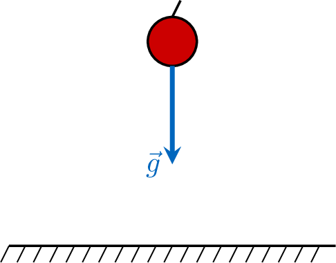
Consider an apple falling from a tree. Let $v(t)$ be its velocity at time $t$, measured along a vertical axis pointing upward; air resistance is neglected. According to Newton's second law, the derivative of the velocity is then the constant acceleration due to gravity:$$ v'(t) = -g \quad (\text{where } g \approx 9.8 \text{ m/s}^2) $$ The velocity function $v$ is a primitive of the constant function $f(t) = -g$.

Determine the general form of the velocity $v(t)$.
If the apple starts from rest at $t=0$, we have the initial condition $v(0) = 0$. Find the unique velocity function.

Answer

The general antiderivatives of $-g$ are of the form $v(t) = -gt + C$.
Using the initial condition: $v(0) = -g(0) + C = 0 \implies C = 0$.
The unique solution is $v(t) = -gt$.

Skills to practice

Understanding Antiderivatives

II.3 Finding Antiderivatives

The process of finding antiderivatives relies on reversing the rules of differentiation. Just as we have a table of derivatives for common functions, we can create a corresponding table of antiderivatives.

Report an error

Proposition — Antiderivatives of Common Functions

$$\begin{array}{|c|c|}\hline \textbf{Function }f(x) & \textbf{An Antiderivative }F(x) \\ \hline k \text{ (a constant)} & k x\\ \hline x^{n}, n \neq-1 & \dfrac{x^{n+1}}{n+1} \\ \hline e^{x} & e^{x} \\ \hline \frac{1}{x} & \ln|x| \\ \hline \cos(x) & \sin(x) \\ \hline \sin(x) & -\cos(x) \\ \hline\end{array}$$

Proof

This table is obtained by reading the table of standard derivatives in reverse.

Example

Find an antiderivative of $f(x)=\frac{1}{x^2}$.

Answer

First, we rewrite the function using a negative exponent: $f(x)=x^{-2}$.
An antiderivative of the power function $f(x)=x^n$ (for $n\neq -1$) is $F(x)=\dfrac{x^{n+1}}{n+1}$. With $n=-2$, we have $$\begin{aligned} F(x) &= \frac{x^{-2+1}}{-2+1} \\ &= \frac{x^{-1}}{-1} \\ &= -\frac{1}{x}\end{aligned}$$

Proposition — Linearity of Integration

Let $u$ and $v$ be two functions with antiderivatives $U$ and $V$, and let $k$ be a constant.

An antiderivative of $u+v$ is $U+V$.
An antiderivative of $ku$ is $kU$.

This allows us to find the antiderivative of a sum of functions term by term.

Example

Find an antiderivative of $f(x)=2x+3$.

Answer

We use the linearity property to find the antiderivative of each term separately.

An antiderivative of $2x$ is $2 \cdot \dfrac{x^2}{2} = x^2$.
An antiderivative of $3$ is $3x$.

Combining these, an antiderivative of $f(x)=2x+3$ is $F(x) = x^2+3x$.

Skills to practice

Finding Antiderivatives of Basic Functions
Finding a Function from Its Derivative and One Value

II.4 Antiderivatives of Composite Functions

Proposition — Antiderivatives of $x \mapsto f(ax + b)$

Let $f$ be a function with an antiderivative $F$ on an interval $I$, and $a$, $b$ real numbers with $a \neq 0$. On every interval on which $ax + b$ stays in $I$, $$\textcolor{colorprop}{x \mapsto \frac{1}{a}\,F(ax + b) \text{ is an antiderivative of } x \mapsto f(ax + b).}$$

Proof

The derivative of $x \mapsto g(ax + b)$ is $x \mapsto a\,g'(ax + b)$. With $g = F$ and $F' = f$: $$\begin{aligned}\left(\frac{1}{a}\,F(ax + b)\right)' &= \frac{1}{a} \times a\,F'(ax + b) &&\text{(derivative of } x \mapsto g(ax + b)\text{)}\\ &= f(ax + b). &&\text{(} F' = f\text{)}\end{aligned}$$ The factor $\dfrac{1}{a}$ compensates the factor $a$ that differentiation brings out.

Example

Determine an antiderivative of each function on the given interval.

$f_1(x) = (2x - 1)^4$ on $\mathbb{R}$.
$f_2(x) = \cos\left(3x + \dfrac{\pi}{4}\right)$ on $\mathbb{R}$.
$f_3(x) = e^{-2x}$ on $\mathbb{R}$.
$f_4(x) = \dfrac{1}{(2x + 1)^2}$ on $\left(-\dfrac{1}{2}, +\infty\right)$.

Answer

Each time, name $f$, an antiderivative $F$ of $f$, and $a$; then $x \mapsto \frac{1}{a}F(ax + b)$ answers.

$f(X) = X^4$, $F(X) = \dfrac{X^5}{5}$, $a = 2$: $F_1(x) = \dfrac{1}{2} \times \dfrac{(2x - 1)^5}{5} = \dfrac{(2x - 1)^5}{10}$.
$f = \cos$, $F = \sin$, $a = 3$: $F_2(x) = \dfrac{1}{3}\sin\left(3x + \dfrac{\pi}{4}\right)$. It is the row $A\cos(\omega t + \varphi)$ of the table of powers and sinusoidal signals ($A = 1$, $\omega = 3$): the proposition on $f(ax + b)$ contains it.
$f = \exp$, $F = \exp$, $a = -2$: $F_3(x) = -\dfrac{1}{2}\,e^{-2x}$.
$f(X) = \dfrac{1}{X^2}$, $F(X) = -\dfrac{1}{X}$ on $(0, +\infty)$, $a = 2$, and $2x + 1 \gt 0$ for $x \gt -\frac{1}{2}$: $F_4(x) = \dfrac{1}{2} \times \left(-\dfrac{1}{2x + 1}\right) = -\dfrac{1}{2(2x + 1)}$.

Check, for the first one: $F_1'(x) = \dfrac{5(2x - 1)^4 \times 2}{10} = (2x - 1)^4$.

Proposition — Antiderivatives of Composite Functions (Reverse Chain Rule)

Let $u$ be a differentiable function of $x$. $$\begin{array}{|c|c|}\hline \textbf{Function }f(x) & \textbf{An Antiderivative }F(x) \\ \hline u'(x) [u(x)]^n, \quad n \neq -1 & \dfrac{[u(x)]^{n+1}}{n+1} \\ \hline \dfrac{u'(x)}{u(x)} & \ln|u(x)| \\ \hline u'(x)e^{u(x)} & e^{u(x)} \\ \hline\end{array}$$

Example

Find an antiderivative of $f(x)=\frac{2x}{x^2+1}$.

Answer

The function $f(x)$ is of the form $\dfrac{u'(x)}{u(x)}$.
Let $u(x) = x^2+1$. Then its derivative is $u'(x) = 2x$.
So, we can write $f(x) = \dfrac{u'(x)}{u(x)}$.
From the table, an antiderivative is $F(x) = \ln|u(x)|$.
Substituting back, we get $F(x) = \ln|x^2+1|$. Since $x^2+1$ is always positive, we can remove the absolute value bars: $$ F(x) = \ln(x^2+1) $$

Skills to practice

Antiderivatives of $f(ax + b)$

II.5 The Fundamental Theorem of Calculus

Theorem — Fundamental Theorem of Calculus

If $f$ is a continuous function on the interval $[a,b]$ and $F$ is any antiderivative of $f$, then: $$ \int_a^b f(x)\,\mathrm{d}x = F(b) - F(a) $$ This result is often written using the notation $\left[ F(x) \right]_a^b = F(b)-F(a)$.

Proof

The theorem states that integration and differentiation are inverse processes. We can understand this by examining the “area function”.

Defining the Area Function: Let's define a function, $A(x)$, as the area under the curve $y=f(t)$ from a fixed starting point $a$ to a variable endpoint $x$: $$ A(x) = \int_a^x f(t) \, \mathrm{d}t. $$ Our goal is to show that the derivative of this area function, $A'(x)$, is simply the original function $f(x)$.
The Area of a Thin Strip: By its definition, the area of a thin vertical strip between $x$ and $x+h$ is the difference between the total area up to $x+h$ and the total area up to $x$: $$ \text{Area of strip} = A(x+h) - A(x). $$
Approximating the Area of the Strip: As shown in the diagram, if the width $h$ is very small, this thin strip is almost a perfect rectangle.
- The width of the rectangle is $h$.
- The height of the rectangle is approximately $f(x)$.
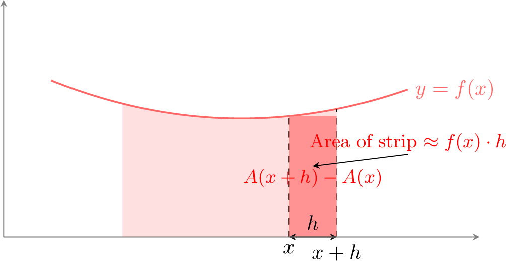
So, we can approximate the strip's area: $$ \text{Area of strip} \approx f(x) \cdot h. $$
Connecting to the Derivative: We now have two expressions for the area of the strip: $$ A(x+h) - A(x) \approx f(x) \cdot h. $$ Dividing both sides by $h$, we get the difference quotient for the function $A(x)$: $$ \frac{A(x+h) - A(x)}{h} \approx f(x). $$
Taking the Limit: This approximation becomes a perfect equality as the width of the strip, $h$, approaches zero. Taking the limit of both sides: $$ \lim_{h\to 0}\frac{A(x+h)-A(x)}{h} = f(x). $$ The expression on the left is, by definition, the derivative of the area function, $A'(x)$: $$ A'(x) = f(x). $$
Finding the Formula: Let $F(x)$ be any antiderivative of $f(x)$. Since all antiderivatives of a function differ only by a constant, we know that: $$ A(x) = F(x) + C $$ for some constant $C$. To find $C$, we can evaluate this at $x=a$: $$ A(a) = \int_a^a f(t)\,\mathrm{d}t = 0 $$ so $$ F(a) + C = 0 \implies C = -F(a). $$ Thus the area function is $A(x) = F(x) - F(a)$.
To find the total area up to $x=b$, we simply evaluate $A(b)$: $$ \int_a^b f(x)\,\mathrm{d}x = A(b) = F(b) - F(a). $$

Remark

This theorem is fundamental because it connects the geometric concept of area (the definite integral) with the algebraic process of antidifferentiation. It gives us a powerful method to calculate exact areas without using the limit of a Riemann sum.

Report an error

Example

Find $\displaystyle \int_0^2 x^2 \mathrm{d}x$.

Answer

Find an antiderivative: An antiderivative of $f(x)=x^2$ is $F(x) = \dfrac{x^3}{3}$.
Apply the Fundamental Theorem: $$\begin{aligned}\displaystyle \int_0^2 x^2 \mathrm{d}x &= \left[ \frac{x^3}{3} \right]_0^2\\ &= F(2) - F(0) \\ &=\frac{2^3}{3} -\frac{0^3}{3}\\ &=\frac{8}{3} - 0 = \frac{8}{3} \end{aligned}$$

This means the exact area under the curve $y=x^2$ over $[0,2]$ is $\dfrac 8 3$.

Theorem — Existence of Antiderivatives

Let $f$ be continuous on an interval $I$, and let $a \in I$. The function $F_a$ defined on $I$ by $$ F_a(x) = \int_a^x f(t)\,\mathrm{d}t $$ is the antiderivative of $f$ that vanishes at $a$: $F_a'=f$ and $F_a(a)=0$. In particular, every function that is continuous on an interval admits antiderivatives.

Skills to practice

Evaluating Definite Integrals and Areas
Evaluating Integrals of Sums

III Techniques of Integration

III.1 Integration by Inspection

Method — Integration by Inspection

A common strategy is to make an educated guess for the antiderivative, differentiate it, and adjust any constant factors. This is often called “integration by inspection” or “guess and check”.

Guess: Look at the function and guess a possible antiderivative.
Differentiate: Differentiate your guess.
Adjust: Compare your result with the original integrand and multiply by a constant factor to correct any discrepancies.

Example

Find the integral of $\sin(3x)$.

Answer

Guess: The integral of $\sin$ is $-\cos$. A good guess for the antiderivative is $F(x) = -\cos(3x)$.
Differentiate: Using the chain rule, the derivative of our guess is $F'(x) = -(-\sin(3x)) \cdot 3 = 3\sin(3x)$.
Adjust: Our result, $3\sin(3x)$, is 3 times larger than the original integrand, $\sin(3x)$. We must therefore divide our initial guess by 3.

The correct antiderivative is $-\dfrac{1}{3}\cos(3x)$. So, $$ \int \sin(3x) \, \mathrm{d}x = -\frac{1}{3}\cos(3x) + C $$

Skills to practice

Finding Antiderivatives by Inspection

III.2 Integration by Substitution

Integration by substitution is a powerful technique that reverses the chain rule for differentiation. It is used when an integrand contains both a function and its derivative.
Consider the integral $\int (2x^3+1)^7 (6x^2) \, \mathrm{d}x$. We can see that the expression contains an “inner function”, $u = 2x^3+1$, and its derivative, $u'(x) = 6x^2$. This structure is a clear indicator for substitution.
Let's define a new variable, $u = 2x^3+1$. Differentiating this with respect to $x$ gives $u'(x)=6x^2$. In differential form, we can write $\mathrm{d}u = 6x^2\,\mathrm{d}x$. Now we can substitute both $u$ and $\mathrm{d}u$ into the original integral: $$\begin{aligned} \int \underbrace{(2x^3+1)^{7}}_{u^{7}} \underbrace{(6x^2)\,\mathrm{d}x}_{\mathrm{d}u} &= \int u^{7}\,\mathrm{d}u \\ &= \frac{1}{8}u^{8}+C\end{aligned}$$ Finally, we substitute back to express the result in terms of $x$: $$ \int (2x^3+1)^7 (6x^2) \, \mathrm{d}x =\frac{1}{8}(2x^3+1)^{8}+C $$

Report an error

Proposition — Integration by Substitution

Indefinite Integral: $$\int f(u(x))u'(x) \, \mathrm{d}x = \int f(u) \, \mathrm{d}u $$
Definite Integral: $$\int_a^b f(u(x))u'(x) \, \mathrm{d}x = \int_{u(a)}^{u(b)} f(u) \, \mathrm{d}u $$

Example

Find $\displaystyle\int_0^1 2x(x^2 + 1)^3\;\mathrm{d}x$.

Answer

Substitution: Let $u = x^2+1$. Then $\mathrm{d}u = 2x\,\mathrm{d}x$.
Change limits:
- When $x=0$, $u = 0^2+1=1$.
- When $x=1$, $u = 1^2+1=2$.
Integrate: We substitute to get a simpler integral in terms of $u$: $$\begin{aligned} \int_0^1 \underbrace{(x^2 + 1)^3}_{u^3} \underbrace{2x\;\mathrm{d}x}_{\mathrm{d}u} &= \int_1^2 u^3 \, \mathrm{d}u \\ &= \left[\frac{u^4}{4}\right]_1^2 \\ &= \frac{2^4}{4} - \frac{1^4}{4} \\ &= 4 - \frac{1}{4}\\ &= \frac{15}{4} \end{aligned}$$

Skills to practice

Integrating by Substitution
Evaluating Definite Integrals by Substitution

III.3 The Antiderivative of $1/\cos^2 x$

Proposition — Antiderivative of $1/\cos^2 x$

On every interval where $\cos x \neq 0$, $$\int \frac{1}{\cos^2 x}\,\mathrm{d}x = \tan x + C.$$ The integrand is also written $\sec^2 x$, or $1 + \tan^2 x$. More generally, for constants $k \neq 0$ and $b$, on every interval where $\cos(kx + b) \neq 0$, $$\int \frac{1}{\cos^2(kx + b)}\,\mathrm{d}x = \frac{1}{k}\tan(kx + b) + C.$$

Proof

For $\cos x \neq 0$, the quotient rule applied to $\tan x = \dfrac{\sin x}{\cos x}$ gives $$\begin{aligned}[t] (\tan x)' &= \frac{\cos x \cos x - \sin x\,(-\sin x)}{\cos^2 x} &&\text{(quotient rule)}\\ &= \frac{\cos^2 x + \sin^2 x}{\cos^2 x}\\ &= \frac{1}{\cos^2 x}. &&(\cos^2 x + \sin^2 x = 1) \end{aligned}$$ Splitting the second fraction instead gives $1 + \dfrac{\sin^2 x}{\cos^2 x} = 1 + \tan^2 x$. So $\tan$ is an antiderivative of $\dfrac{1}{\cos^2 x}$ on every interval where $\cos x \neq 0$. For the composite, the chain rule with $u(x) = kx + b$ and $u'(x) = k$ gives $$\begin{aligned}[t] \left(\frac{1}{k}\tan(kx + b)\right)' &= \frac{1}{k} \times k \times \frac{1}{\cos^2(kx + b)} &&\text{(chain rule)}\\ &= \frac{1}{\cos^2(kx + b)}. \end{aligned}$$

Example

Find $\displaystyle\int \frac{1}{\cos^2(3x - 1)}\,\mathrm{d}x$.
Calculate $\displaystyle\int_0^{\pi/6} \frac{1}{\cos^2(2x)}\,\mathrm{d}x$.

Answer

The integrand has the form $\dfrac{1}{\cos^2(kx + b)}$ with $k = 3$ and $b = -1$. On every interval where $\cos(3x - 1) \neq 0$, $$\int \frac{1}{\cos^2(3x - 1)}\,\mathrm{d}x = \frac{1}{3}\tan(3x - 1) + C.$$ Check: $\left(\dfrac{1}{3}\tan(3x - 1)\right)' = \dfrac{1}{3} \times 3 \times \dfrac{1}{\cos^2(3x - 1)} = \dfrac{1}{\cos^2(3x - 1)}$.
For $0 \le x \le \dfrac{\pi}{6}$, $0 \le 2x \le \dfrac{\pi}{3}$, so $\cos(2x) \neq 0$ on the whole interval. With $k = 2$, $$\begin{aligned}[t] \int_0^{\pi/6} \frac{1}{\cos^2(2x)}\,\mathrm{d}x &= \left[\frac{1}{2}\tan(2x)\right]_0^{\pi/6} &&\text{(antiderivative of } 1/\cos^2(kx + b)\text{)}\\ &= \frac{1}{2}\tan\frac{\pi}{3} - \frac{1}{2}\tan 0 &&\\ &= \frac{\sqrt{3}}{2}. &&\Big(\tan\frac{\pi}{3} = \sqrt{3}\Big) \end{aligned}$$

Skills to practice

Integrating $1/\cos^2(kx + b)$

IV Numerical Integration

IV.1 The Trapezoidal Rule

When an antiderivative is hard or impossible to express with elementary functions, a definite integral can be estimated numerically. The trapezoidal rule approximates the area under $y=f(x)$ by trapezia of equal width.

Report an error

Proposition — The Trapezoidal Rule

Divide $[a,b]$ into $n$ strips of width $h=\dfrac{b-a}{n}$, with points $x_0=a,\,x_1,\dots,x_n=b$. Then $$ \int_a^b f(x)\,\mathrm{d}x \approx \frac{h}{2}\Big[\,f(x_0)+2f(x_1)+2f(x_2)+\dots+2f(x_{n-1})+f(x_n)\,\Big]. $$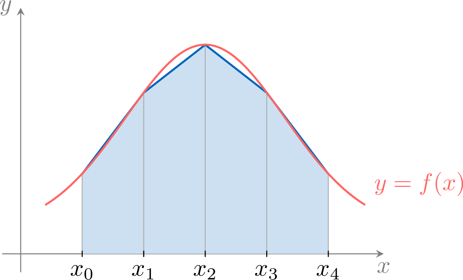

Proof

A trapezium with parallel sides $p,q$ and width $h$ has area $\frac{h}{2}(p+q)$. On the strip $[x_k,x_{k+1}]$ the two parallel sides are the ordinates $f(x_k)$ and $f(x_{k+1})$, so its area is $\frac{h}{2}\big(f(x_k)+f(x_{k+1})\big)$.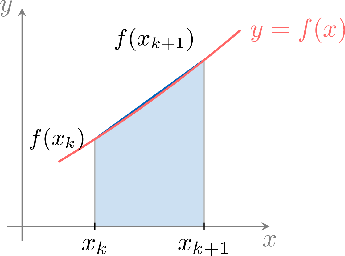

Summing the $n$ strips and expanding, $$\begin{aligned} \int_a^b f(x)\,\mathrm{d}x &\approx \sum_{k=0}^{n-1}\tfrac{h}{2}\big(f(x_k)+f(x_{k+1})\big)\\ &= \tfrac{h}{2}\big[(f(x_0){+}f(x_1))+(f(x_1){+}f(x_2))+\dots+(f(x_{n-1}){+}f(x_n))\big]. \end{aligned}$$ Each interior ordinate $f(x_1),\dots,f(x_{n-1})$ belongs to two consecutive trapezia, so appears twice; the endpoints $f(x_0)$ and $f(x_n)$ appear once. Regrouping gives the formula $$ \int_a^b f(x)\,\mathrm{d}x \approx \tfrac{h}{2}\big[f(x_0)+2f(x_1)+\dots+2f(x_{n-1})+f(x_n)\big]. $$

Example

Estimate $\displaystyle\int_0^4 \sqrt{x}\,\mathrm{d}x$ using the trapezoidal rule with $n=4$ strips.

Answer

Here $h=\frac{4-0}{4}=1$, with $x_0,\dots,x_4=0,1,2,3,4$ and $f(x)=\sqrt{x}$: $$ \begin{array}{c|ccccc} x & 0 & 1 & 2 & 3 & 4 \\ \hline f(x) & 0 & 1 & \sqrt2 & \sqrt3 & 2 \end{array} $$ $$\begin{aligned} \int_0^4\!\sqrt{x}\,\mathrm{d}x &\approx \tfrac{1}{2}\big[0+2(1)+2\sqrt2+2\sqrt3+2\big] &&\text{(trapezoidal rule)}\\ &= 2+\sqrt2+\sqrt3 \approx 5.15 &&\text{(exact: }\tfrac{16}{3}\approx5.33) \end{aligned}$$ As $\sqrt{x}$ is concave, the trapezia lie below the curve, so this underestimates.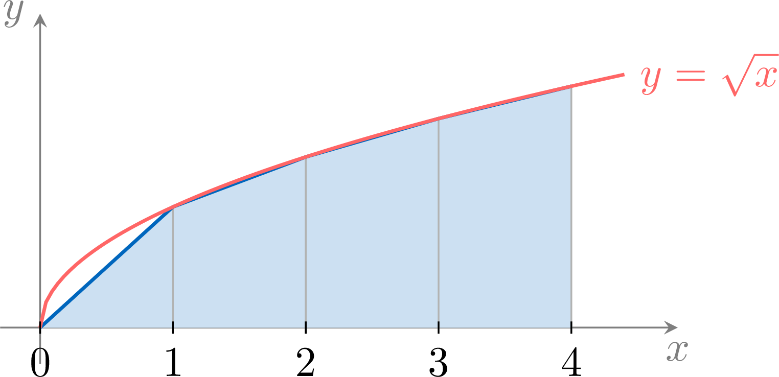

Example

A lake is $120$ m long. Its width $w$, in metres, is measured every $20$ m along a straight line that joins its two ends: $$ \begin{array}{c|ccccccc} x\ (\text{m}) & 0 & 20 & 40 & 60 & 80 & 100 & 120 \\ \hline w\ (\text{m}) & 0 & 38 & 52 & 60 & 55 & 41 & 0 \end{array} $$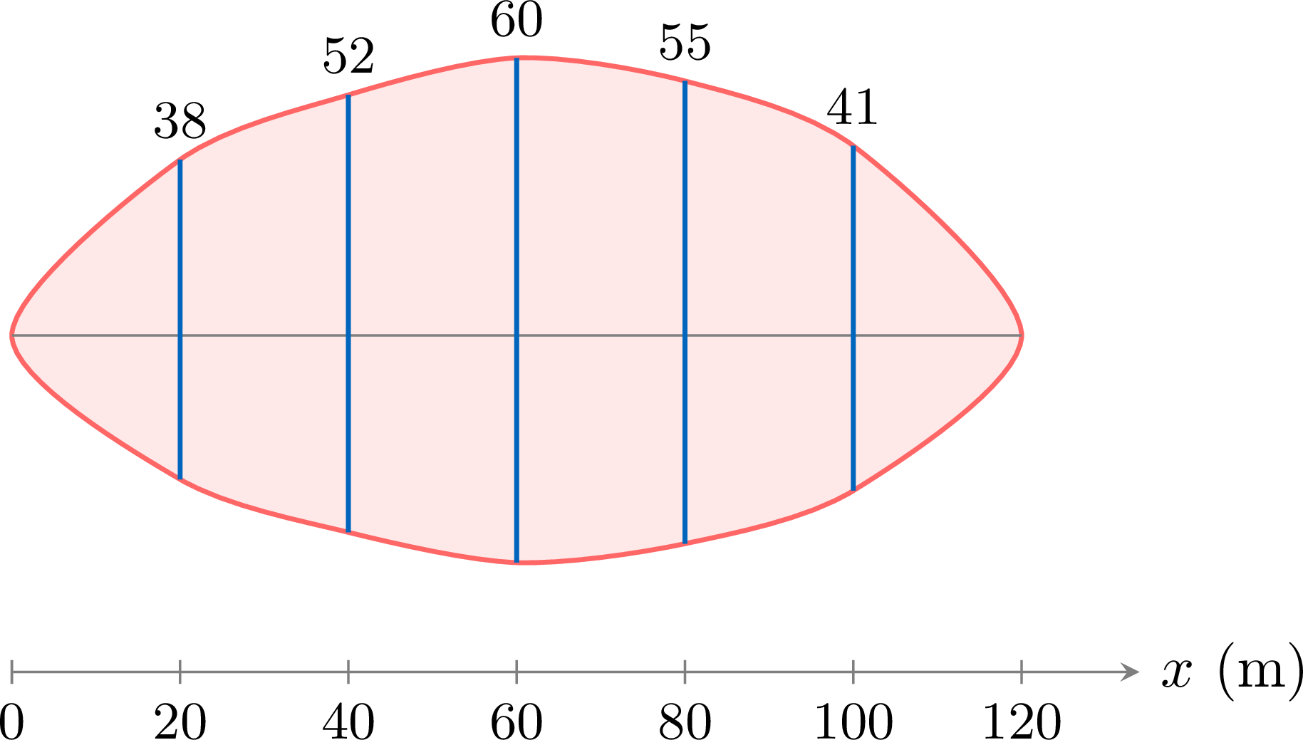

The area of the lake is $\displaystyle\int_0^{120} w(x)\,\mathrm{d}x$, where $w(x)$ is the width at the distance $x$ from the first end; no formula gives $w(x)$. Use the trapezoidal rule, with the strips of the table, to estimate the area of the lake.

Answer

The table gives $n = 6$ strips of width $h = 20$ m, with $x_0 = 0$, $x_1 = 20$, …, $x_6 = 120$. The trapezoidal rule counts the two end widths once and the five inside widths twice: $$\begin{aligned}[t] \int_0^{120} w(x)\,\mathrm{d}x &\approx \frac{h}{2}\Big[w(x_0) + 2\big(w(x_1) + \dots + w(x_5)\big) + w(x_6)\Big] &&\text{(trapezoidal rule)}\\ &= \frac{20}{2}\Big[0 + 2(38 + 52 + 60 + 55 + 41) + 0\Big]\\ &= 10 \times 2 \times 246\\ &= 4920. \end{aligned}$$ The area of the lake is about $4920$ m$^2$. Only the measured widths are used: the rule needs the values of the function at the points of the subdivision, not a formula.

Skills to practice

Applying the Trapezoidal Rule
Estimating Integrals and Judging the Estimate

IV.2 Definite Integrals with Technology

Method — Evaluating a Definite Integral with Technology

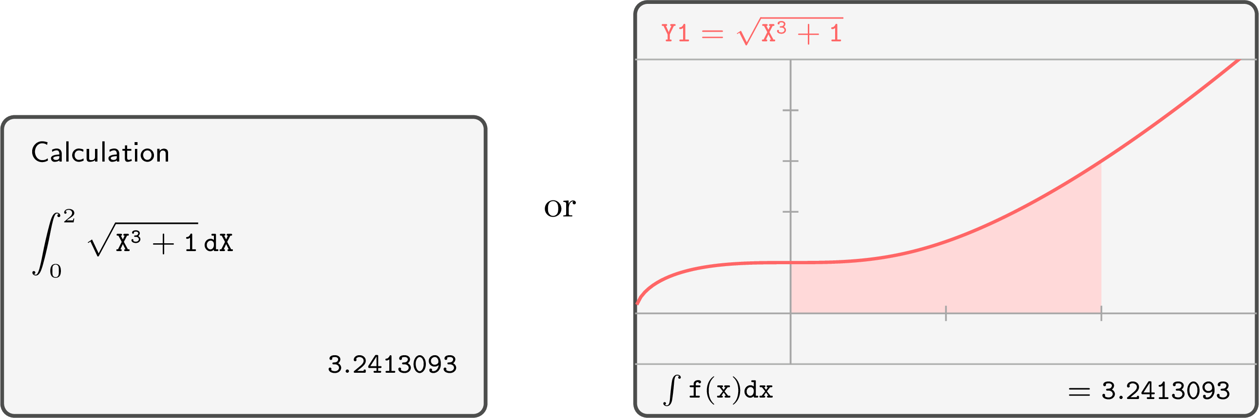
A graphing calculator evaluates a definite integral $\displaystyle\int_a^b f(x)\,\mathrm{d}x$ numerically, even when no formula gives its value. It offers two tools: the integral template of the calculation screen, where the integrand and the two bounds are typed, and the integral tool of the graph screen, which asks for the lower bound, then the upper bound, and shades the region. Both return a decimal approximation of the signed area.

Write the integral first, on paper: the integrand, the bounds and the differential, $\displaystyle\int_a^b f(x)\,\mathrm{d}x$. This expression is the method; the calculator only evaluates it. For an area, a sketch first shows where the curve lies above or below the $x$-axis between $a$ and $b$.
Set the angle unit to radians when $f(x)$ contains $\sin$, $\cos$ or $\tan$.
Enter the integral: the integrand, written with the variable $X$ of the calculator, then the lower bound $a$ and the upper bound $b$, in this order.
Report the value to 3 significant figures, unless the question asks for another accuracy.
Interpret the sign: the value is a signed area. It is the area of the region only when $f(x) \ge 0$ on $[a, b]$; when $f(x) \le 0$ on the whole of $[a, b]$, the area is $-\displaystyle\int_a^b f(x)\,\mathrm{d}x$. When the curve crosses the $x$-axis between $a$ and $b$, the area of the region is $\displaystyle\int_a^b |f(x)|\,\mathrm{d}x$, evaluated with the absolute-value function of the calculator; alternatively, the zeros of $f$ in $[a, b]$ are found with the zero tool, $[a, b]$ is split at these zeros, and the absolute values of the integrals over the pieces, from $a$ to the first zero and from the last zero to $b$ included, are added.

The mock-up evaluates $\displaystyle\int_0^2 \sqrt{x^3+1}\,\mathrm{d}x$ with each tool; the window of the graph screen is $-1 \le x \le 3$, $-1 \le y \le 5$.

Example

The region $R$ is bounded by the curve $y = \sqrt{x^3+1}$, the $x$-axis and the lines $x = 0$ and $x = 2$.

Write down an integral that gives the area of $R$.
Find the area of $R$ with technology.
Check that this value is plausible, with a rectangle that lies under the curve and a rectangle that contains $R$.

Answer

For $0 \le x \le 2$, $x^3 + 1 \ge 1$, so $\sqrt{x^3+1} \ge 1 > 0$: the curve lies above the $x$-axis, and the area of $R$ is $$\mathcal{A} = \int_0^2 \sqrt{x^3+1}\,\mathrm{d}x.$$
The integral template, with the integrand $\sqrt{X^3+1}$ and the bounds $0$ and $2$, displays $3.2413093$; the integral tool of the graph screen, with the lower bound $0$ and the upper bound $2$, displays the same value. The area of $R$ is $\mathcal{A} \approx 3.24$ square units.
On $[0, 2]$, $x^3 + 1$ increases, so $f(x) = \sqrt{x^3+1}$ increases from $f(0) = 1$ to $f(2) = \sqrt{9} = 3$. The rectangle of width $2$ and height $f(0)$ lies under the curve, and the rectangle of width $2$ and height $f(2)$ contains $R$: $$\begin{aligned}[t] 2 \times f(0) &\le \mathcal{A} \le 2 \times f(2) &&\text{(one rectangle below, one rectangle above)}\\ 2 &\le \mathcal{A} \le 6. \end{aligned}$$ The value $3.24$ lies between $2$ and $6$.

Example

Let $f(x) = x^3 - 4x$.

Evaluate $\displaystyle\int_{-1}^{3} f(x)\,\mathrm{d}x$ with technology.
Find the area of the region bounded by the curve of $f$, the $x$-axis and the lines $x = -1$ and $x = 3$.
Explain why the two values differ.

Answer

The integral template, with the integrand $X^3 - 4X$ and the bounds $-1$ and $3$, displays $4$: to 3 significant figures, $$\int_{-1}^{3} f(x)\,\mathrm{d}x \approx 4.00.$$
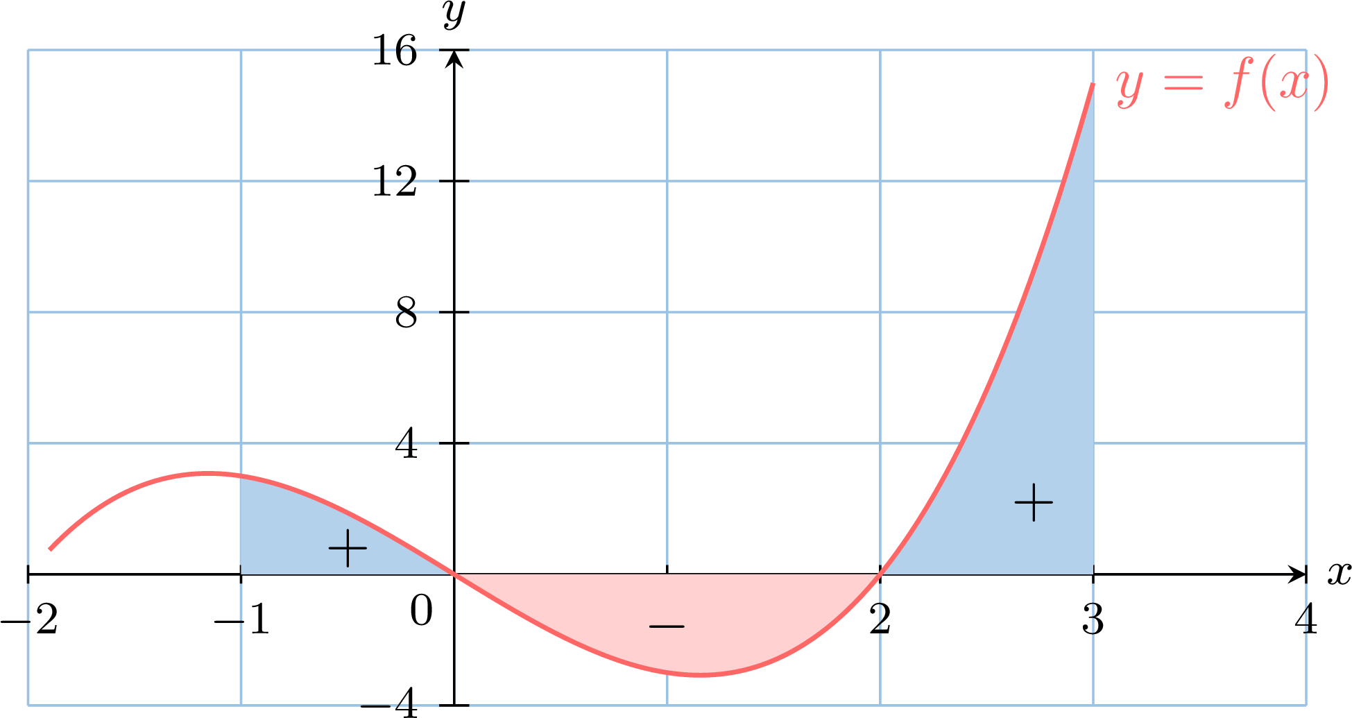
The zero tool, in the window $-2 \le x \le 3.5$, $-5 \le y \le 16$, displays the zeros $-2$, $0$ and $2$; the factorisation $f(x) = x(x - 2)(x + 2)$ confirms them. In $[-1, 3]$ the curve crosses the $x$-axis at $0$ and at $2$: it lies above the axis on $[-1, 0]$ and on $[2, 3]$, below it on $[0, 2]$. For the three pieces, the template displays $1.75$, $-4$ and $6.25$: $\displaystyle\int_{-1}^{0} f(x)\,\mathrm{d}x \approx 1.75$, $\displaystyle\int_{0}^{2} f(x)\,\mathrm{d}x \approx -4$ and $\displaystyle\int_{2}^{3} f(x)\,\mathrm{d}x \approx 6.25$. Each part counts positively in the area: $$\begin{aligned}[t] \mathcal{A} &= \left|\int_{-1}^{0} f(x)\,\mathrm{d}x\right| + \left|\int_{0}^{2} f(x)\,\mathrm{d}x\right| + \left|\int_{2}^{3} f(x)\,\mathrm{d}x\right| &&\text{(split at the zeros)}\\ &\approx 1.75 + 4 + 6.25 &&\text{(values displayed)}\\ &\approx 12.0. \end{aligned}$$ The template with the integrand $|X^3 - 4X|$ displays $12$ directly. The area of the region is about $12.0$ square units.
The integral is a signed area: the part below the axis, on $[0, 2]$, counts negatively, so $1.75 - 4 + 6.25 = 4$. The area counts every part positively: $1.75 + 4 + 6.25 = 12$.

Skills to practice

Setting Up an Integral for the Calculator
Evaluating Integrals and Areas with Technology

V Going further

Skills to practice

Solving Problems
Quiz