International Baccalaureate · DP 2: Analysis and Approaches HL
Systems of Linear Equations
I
Linear Systems and Their Solutions
I.1
Two Equations in Two Unknowns
Recappreviously studied — click to reread
Method — Solving by Elimination
- Write both equations in the form \(ax + by = c\), with the unknowns lined up.
- Choose the unknown to eliminate. If needed, multiply one equation, or both, by nonzero numbers so that the two coefficients of this unknown become opposite (or equal).
- Add the two equations when these coefficients are opposite, subtract them when they are equal: the chosen unknown disappears.
- Solve the equation obtained, which has only one unknown.
- Back-substitute the value found in one of the original equations to find the other unknown.
- Check the pair in both original equations, then conclude. When the combinations lead to one value of each unknown, they only show that no other pair is possible; the check shows that this pair is indeed a solution. When both unknowns disappear, the Method “Recognising the Case While Solving” applies.
Proposition — Number of Solutions of a System
Consider a system whose equations can be rearranged as \(y = m_1x + c_1\) and \(y = m_2x + c_2\), where \(m_1\) and \(m_2\) are the gradients (also called slopes) of the two lines. - If \(m_1 \neq m_2\), the lines are intersecting: the system has exactly one solution.
- If \(m_1 = m_2\) and \(c_1 \neq c_2\), the lines are parallel and distinct: the system has no solution.
- If \(m_1 = m_2\) and \(c_1 = c_2\), the lines are coincident (they are the same line): the system has infinitely many solutions, all the pairs \((x, m_1x + c_1)\).
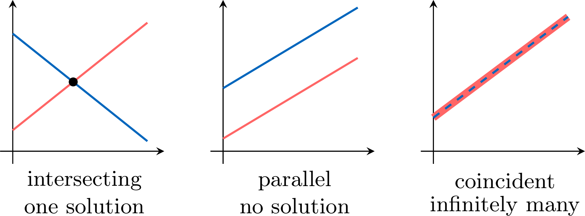
A solution \((x, y)\) satisfies \(y = m_1x + c_1\) and \(y = m_2x + c_2\), so the two expressions of \(y\) are equal: $$\begin{aligned}[t] m_1x + c_1 &= m_2x + c_2 && \text{(both are equal to } y\text{)} \\
m_1x - m_2x + c_1 &= c_2 && \text{(subtract } m_2x \text{ from both sides)} \\
m_1x - m_2x &= c_2 - c_1 && \text{(subtract } c_1 \text{ from both sides)} \\
(m_1 - m_2)x &= c_2 - c_1 && \text{(factorise by } x\text{)} \end{aligned}$$
- If \(m_1 \neq m_2\), then \(m_1 - m_2 \neq 0\), and dividing by it gives the single value \(x = \dfrac{c_2 - c_1}{m_1 - m_2}\), then the single value \(y = m_1x + c_1\). For this \(x\) the two expressions of \(y\) are equal, so this pair satisfies both equations: exactly one solution.
- If \(m_1 = m_2\), the last equation reads \(0 \times x = c_2 - c_1\). When \(c_1 \neq c_2\), it is false for every \(x\): no solution. When \(c_1 = c_2\), the two equations are the same equation, and every pair \((x, m_1x + c_1)\) satisfies both: infinitely many solutions.
Method — Recognising the Case While Solving
When substitution or elimination makes both unknowns disappear: - a false equality, such as \(0 = -2\), means that no pair is a solution: the lines are parallel and distinct;
- an equality that is always true, such as \(0 = 0\), means that the two equations describe the same line: the solutions are all the pairs \((x, y)\) satisfying one of the equations, written \(y = mx + c\).
Skills to practice
- Setting Up Linear Systems
I.2
Linear Equations and Systems
Systems of two linear equations in two unknowns are solved by substitution or by elimination. We now look at more general systems and how they can be represented using augmented matrices. This is a first step into the branch of mathematics called linear algebra, which underpins much of modern technology (computer science, engineering, physics, economics, etc.).
Definition — Linear Equation
A linear equation in the variables \(x_1, x_2, \dots, x_n\) is an equation that can be written in the form $$ a_1x_1 + a_2x_2 + \dots + a_nx_n = b $$ where \(a_1, a_2, \dots, a_n\) and \(b\) are constants. A solution to the equation is an assignment of one value to each variable — an ordered tuple — that makes the equation true. Definition — System of Linear Equations
A system of \(m\) linear equations in \(n\) unknowns, \(x_1,x_2,\dots,x_n\), can be written in the form $$\left\{\begin{array}{rcrcrcrcl} a_{11}x_1 & + & a_{12}x_2 &+& \dots &+ & a_{1n}x_n &=& b_1 \\
a_{21}x_1 & + & a_{22}x_2 &+& \dots &+ & a_{2n}x_n &=& b_2 \\
\vdots & & \vdots & & \dots & & \vdots & & \vdots \\
a_{m1}x_1 & + & a_{m2}x_2 &+& \dots &+ & a_{mn}x_n &=& b_m \\
\end{array}\right.$$ A solution to the system is an assignment of one value to each variable — an ordered tuple — that satisfies every equation in the system. Definition — Consistent/Inconsistent System
A system of linear equations is: - consistent if it has at least one solution,
- inconsistent if it has no solution.
Example
Show that the following system of equations is inconsistent: $$\left\{\begin{array}{rcrcr} x & + & y & = & 3 \\
2x & + & 2y & = & 8 \end{array}\right.$$
If we take the second equation and divide it by 2, we get $$ \frac{2x+2y}{2} = \frac{8}{2} \implies x+y = 4. $$ The system is therefore equivalent to $$\left\{\begin{array}{rcrcr} x & + & y & = & 3 \\
x & + & y & = & 4 \end{array}\right.$$ This is a contradiction, since \(x+y\) cannot be equal to both 3 and 4. Therefore, the system has no solution and is inconsistent. 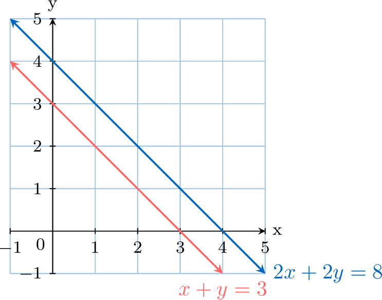
Skills to practice
- Recognising Linear Equations and Their Solutions
I.3
Representations of Solution Sets
The set of all solutions to a system of linear equations can be represented in several ways. The most common forms are:
- the Cartesian (implicit) equation,
- the parametric form,
- the vector form.
Example
Consider the linear equation \(2x+y=1\). Geometrically, its solution set is a line in the 2D plane. - Parametric Form
We introduce a parameter \(t\) and let \(x=t\). Substituting into the equation, $$ 2t+y=1 \implies y=1-2t. $$ The general solution in parametric form is $$ \boldsymbol{(x, y) = (t, 1-2t)}, \quad t \in \mathbb{R}. $$ - Vector Form
We write the solution as a vector equation: $$ \begin{aligned} \begin{pmatrix} x \\ y \end{pmatrix} &= \begin{pmatrix} t \\ 1-2t \end{pmatrix} \\ &= \begin{pmatrix} 0 \\ 1 \end{pmatrix} + \begin{pmatrix} t \\ -2t \end{pmatrix} \\ &= \underbrace{\begin{pmatrix} 0 \\ 1 \end{pmatrix}}_{\text{position vector}} + t \underbrace{\begin{pmatrix} 1 \\ -2 \end{pmatrix}}_{\text{direction vector}}. \end{aligned} $$ Any point \(\begin{pmatrix} x \\ y \end{pmatrix}\) on the line is obtained by starting from the fixed point \((0,1)\) and moving \(t\) times along the direction vector \(\begin{pmatrix}1\\-2\end{pmatrix}\).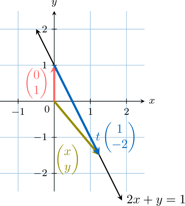
Proposition — Geometric Interpretation of Solutions in 3D
In a 3-dimensional space with variables \((x, y, z)\), for equations whose variable coefficients are not all zero: - The solution set of a single linear equation is a plane. The solutions can be described using two parameters.
- The solution set of a system of two equations describing non-parallel, non-coincident planes is a line: the intersection of the two planes. The solutions can be described using one parameter.
Example
Consider the equation \(x + 2y + 3z = 6\). Geometrically, this represents a plane in 3D space. - Parametric Form
We need two parameters. Let \(y=s\) and \(z=t\). Then $$ x + 2s + 3t = 6 \implies x = 6 - 2s - 3t. $$ The general solution in parametric form is $$ \boldsymbol{(x, y, z) = (6 - 2s - 3t, s, t)}, \quad s,t \in \mathbb{R}. $$ - Vector Form
We write the solution as a vector equation: $$ \begin{aligned} \begin{pmatrix} x \\ y \\ z \end{pmatrix} &= \begin{pmatrix} 6 - 2s - 3t \\ s \\ t \end{pmatrix} \\ &= \begin{pmatrix} 6 \\ 0 \\ 0 \end{pmatrix} + s \begin{pmatrix} -2 \\ 1 \\ 0 \end{pmatrix} + t \begin{pmatrix} -3 \\ 0 \\ 1 \end{pmatrix} \\ &= \underbrace{\begin{pmatrix} 6 \\ 0 \\ 0 \end{pmatrix}}_{\text{position vector}} + s \underbrace{\begin{pmatrix} -2 \\ 1 \\ 0 \end{pmatrix}}_{\text{direction vector 1}} + t \underbrace{\begin{pmatrix} -3 \\ 0 \\ 1 \end{pmatrix}}_{\text{direction vector 2}}. \end{aligned} $$ Any point on the plane is obtained by starting at \((6,0,0)\) and moving along a combination of the two direction vectors.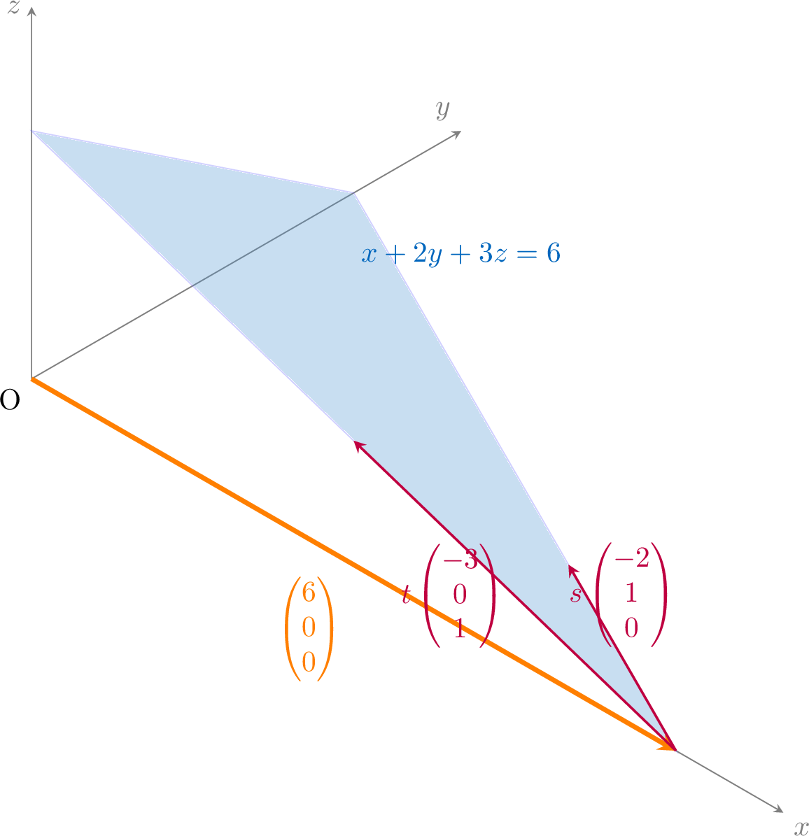
Example
Consider the system $$\left\{\begin{array}{rcrcrcl} x &+& y &+& z &=& 3 \\
x &-& y &+& 2z &=& 2 \end{array}\right.$$ Geometrically, these are two planes in 3D. If they are not parallel and not the same plane, their solution set is the line where they intersect. - Parametric Form
Add the two equations to eliminate \(y\): $$ (x+y+z) + (x-y+2z) = 3+2 \implies 2x + 3z = 5. $$ Introduce a parameter \(t\) by letting \(z=t\): $$ 2x + 3t = 5 \implies x = \frac{5}{2} - \frac{3}{2}t. $$ Substitute \(x\) and \(z\) into the first equation to find \(y\): $$ \left(\frac{5}{2} - \frac{3}{2}t\right) + y + t = 3 \implies y = \frac{1}{2} + \frac{1}{2}t. $$ The parametric solution is $$ \boldsymbol{(x, y, z) = \left(\frac{5}{2} - \frac{3}{2}t,\ \frac{1}{2} + \frac{1}{2}t,\ t\right)}, \quad t \in \mathbb{R}. $$ - Vector Form
We write the solution as a vector equation: $$ \begin{aligned} \begin{pmatrix} x \\ y \\ z \end{pmatrix} &= \begin{pmatrix} 5/2 - 3/2 t \\ 1/2 + 1/2 t \\ t \end{pmatrix} \\ &= \underbrace{\begin{pmatrix} 5/2 \\ 1/2 \\ 0 \end{pmatrix}}_{\text{position vector}} + t \underbrace{\begin{pmatrix} -3/2 \\ 1/2 \\ 1 \end{pmatrix}}_{\text{direction vector}}. \end{aligned} $$ This is the vector equation of the line of intersection.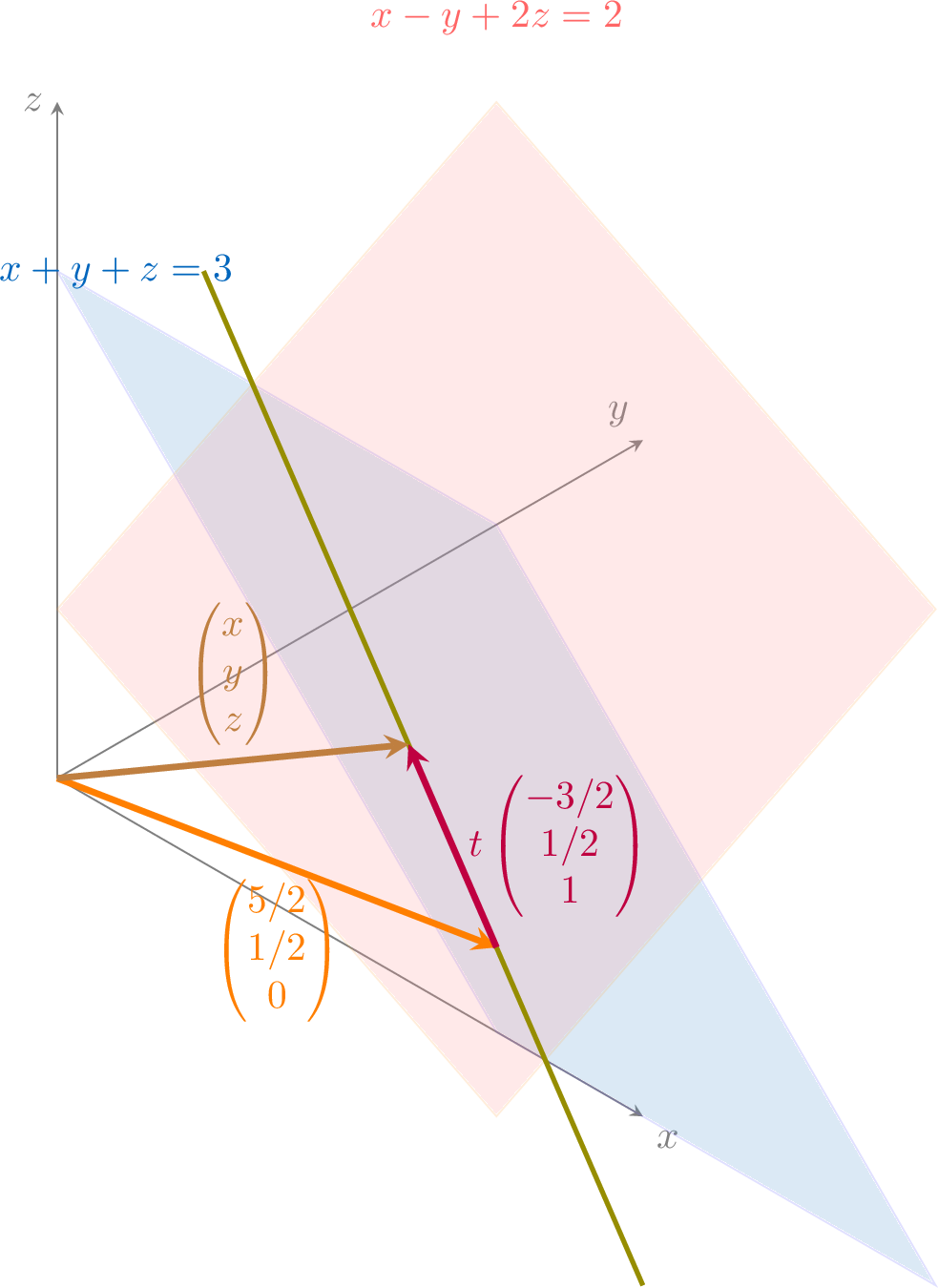
Skills to practice
- Identifying Parametric Solution Sets
II
Row Reduction
II.1
Augmented Matrices
An augmented matrix is a compact way to record a linear system so that we can perform fast, systematic calculations.
Definition — Augmented Matrix
A system of \(m\) linear equations in \(n\) unknowns can be represented by a rectangular array of numbers called an augmented matrix. For the general system $$\left\{\begin{array}{rcrcrcrcl} a_{11}x_1 & + & a_{12}x_2 &+& \dots &+ & a_{1n}x_n &=& b_1 \\
a_{21}x_1 & + & a_{22}x_2 &+& \dots &+ & a_{2n}x_n &=& b_2 \\
\vdots & & \vdots & & \dots & & \vdots & & \vdots \\
a_{m1}x_1 & + & a_{m2}x_2 &+& \dots &+ & a_{mn}x_n &=& b_m \\
\end{array}\right.$$ the augmented matrix is $$ \left[ \begin{array}{cccc|c} a_{11} & a_{12} & \dots & a_{1n} & b_1 \\
a_{21} & a_{22} & \dots & a_{2n} & b_2 \\
\vdots & \vdots & \ddots & \vdots & \vdots \\
a_{m1} & a_{m2} & \dots & a_{mn} & b_m \end{array} \right]. $$ Example
Write down the augmented matrix for the following system of linear equations: $$\left\{\begin{array}{rcrcrcr} 2x &-& y &+& z &=& -1 \\
x & & &+& 3z &=& 4 \\
-x &+& 2y &-& z &=& 0 \end{array}\right.$$
The system has three variables (\(x, y, z\)) and three equations. Each column corresponds to the coefficients of one variable. If a variable is missing from an equation, its coefficient is 0.
The augmented matrix is $$ \left[ \begin{array}{ccc|c} 2 & -1 & 1 & -1 \\ 1 & 0 & 3 & 4 \\ -1 & 2 & -1 & 0 \end{array} \right]. $$
The augmented matrix is $$ \left[ \begin{array}{ccc|c} 2 & -1 & 1 & -1 \\ 1 & 0 & 3 & 4 \\ -1 & 2 & -1 & 0 \end{array} \right]. $$
Skills to practice
- Writing Augmented Matrices
- Writing Systems from Augmented Matrices
II.2
Elementary Row Operations
From our work with simultaneous equations, we know we can perform certain operations without changing the solution set of the system:
- Interchange the equations
For example, \(\left\{ \begin{array}{rcrcrc} 2x&+& y &=& -1 \\ x &-& 3y &=& 2 \\ \end{array}\right.\) has the same solutions as \(\left\{ \begin{array}{rcrcrc} x &-& 3y &=& 2 \\ 2x&+& y &=& -1 \qquad \scriptstyle (R_1 \leftrightarrow R_2) \end{array}\right.\) - Replace an equation by a non-zero multiple of itself
For example, \(\left\{ \begin{array}{rcrcrc} x &-& 3y &=& 2 \\ 2x&+& y &=& -1 \end{array}\right.\) has the same solutions as \(\left\{ \begin{array}{rcrcrc} 2x &-& 6y &=& 4 \qquad \scriptstyle (R_1 \leftarrow 2R_1) \\ 2x&+& y &=& -1 \end{array}\right.\) - Replace an equation by the sum of itself and a multiple of another equation
For example, \(\left\{ \begin{array}{rcrcrc} x &-& 3y &=& 2 \\ 2x&+& y &=& -1 \end{array}\right.\) has the same solutions as \(\left\{ \begin{array}{rcrcrc} x &-& 3y &=& 2 \\ & & 7y &=& -5 \qquad \scriptstyle (R_2 \leftarrow R_2 - 2R_1) \end{array}\right.\), as shown by $$\begin{array}{rcrl} 2x + y &=& -1 &\scriptstyle R_2 \\ -2x + 6y &=& -4& \scriptstyle -2 R_1 \\ \hline 7y &=& -5 & \scriptstyle R_2-2R_1 \end{array}$$
Proposition — Elementary Row Operations
To solve a system using its augmented matrix, we use elementary row operations to transform the matrix into a simpler, equivalent form. These operations do not change the solution set of the system. - Interchange two rows (\(R_i \leftrightarrow R_j\)).
- Multiply a row by a non-zero constant (\(R_i \leftarrow kR_i\)).
- Add a multiple of one row to another row (\( R_i \leftarrow R_i + kR_j\)).
Skills to practice
- Performing Row Operations on Systems
- Performing Row Operations on Matrices
II.3
Gaussian Elimination
Gaussian elimination is the process of using elementary row operations to systematically solve a system of linear equations. The aim is to transform the augmented matrix into row-echelon form.
Definition — Pivot and Row-Echelon Form
In a matrix, the pivot of a non-zero row is its first non-zero entry (reading from the left). The matrix is in row-echelon form when: - every zero row lies below all the non-zero rows;
- the pivot of each non-zero row lies strictly to the right of the pivot of the row above.
Method — Solving a System with Gaussian Elimination
- Augmented Matrix: Write the system of linear equations as an augmented matrix.

- Row-Echelon Form: Use row operations to create a “triangle” of zeros in the bottom-left corner of the matrix (zeros below each pivot).

- Reduced Row-Echelon Form (optional): Continue using row operations to create zeros above the pivots and make each pivot equal to 1. The coefficient matrix becomes the identity matrix (when the system has a unique solution).

- Read the solution: The final matrix gives the solution directly (the cases without a unique solution are analysed separately):

Example
Use Gaussian elimination to solve: $$\left\{\begin{array}{rcrcr} x & + & y & = & -1 \\
2x & + & 4y & = & 6 \end{array}\right.$$
$$ \begin{aligned} & \left\{\begin{array}{rcrcr} x & + & y & = & -1 \\
2x & + & 4y & = & 6 \end{array}\right.\\
\sim\;&\left[ \begin{array}{cc|c} 1 & 1 & -1 \\
2 & 4 & 6 \end{array} \right] &&\scriptstyle(\text{write the augmented matrix})\\
\sim\;&\left[ \begin{array}{cc|c} 1 & 1 & -1 \\
0 & 2 & 8 \end{array} \right] \begin{array}{l} \\
\scriptstyle R_2 \leftarrow R_2 - 2R_1 \end{array} &&\scriptstyle(\text{create a zero below the pivot})\\
\sim\;&\left[ \begin{array}{cc|c} 1 & 1 & -1 \\
0 & 1 & 4 \end{array} \right] \begin{array}{l} \\
\scriptstyle R_2 \leftarrow \frac{1}{2}R_2 \end{array} &&\scriptstyle(\text{make the pivot in Row 2 equal to 1})\\
\sim\;&\left[ \begin{array}{cc|c} 1 & 0 & -5 \\
0 & 1 & 4 \end{array} \right] \begin{array}{l} \scriptstyle R_1 \leftarrow R_1-R_2 \\
\; \end{array} &&\scriptstyle(\text{create a zero above the pivot in Row 2}) \\
\text{i.e.\ }&\left\{\begin{array}{rcrcr} x & & & = & -5 \\
& & y & = & 4 \end{array}\right. &&\scriptstyle(\text{read off the solution}) \end{aligned} $$ So the solution of the system is \((-5, 4)\).
Example
Solve the following system using Gaussian elimination: $$\left\{\begin{array}{rcrcrcl} x &+& y &+& z &=& 6 \\
2x &-& y &+& z &=& 3 \\
x &+& 2y &-& z &=& 2 \end{array}\right.$$
$$\begin{aligned} \,&\left[\begin{array}{ccc|c} 1 & 1 & 1 & 6\\
2 & -1 & 1 & 3\\
1 & 2 & -1 & 2 \end{array}\right]\\
\sim&\left[\begin{array}{ccc|c} 1 & 1 & 1 & 6\\
0 & -3 & -1 & -9\\
0 & 1 & -2 & -4 \end{array}\right] \begin{array}{l} \\
\scriptstyle R_2\leftarrow R_2-2R_1\\
\scriptstyle R_3\leftarrow R_3-R_1 \end{array}\\
\sim&\left[\begin{array}{ccc|c} 1 & 1 & 1 & 6\\
0 & 1 & -2 & -4\\
0 & -3 & -1 & -9 \end{array}\right] \begin{array}{l} \\
\scriptstyle R_2\leftrightarrow R_3\\
\\
\end{array}\\
\sim&\left[\begin{array}{ccc|c} 1 & 1 & 1 & 6\\
0 & 1 & -2 & -4\\
0 & 0 & -7 & -21 \end{array}\right] \begin{array}{l} \\
\\
\scriptstyle R_3\leftarrow R_3+3R_2 \end{array} \end{aligned}$$ The matrix is now in row-echelon form, and we solve by back-substitution, from the bottom row up:
- Row 3: \(-7z = -21\), so \(z = 3\);
- Row 2: \(y - 2z = -4\), so \(y = -4 + 2\times 3 = 2\);
- Row 1: \(x + y + z = 6\), so \(x = 6 - 2 - 3 = 1\).
Skills to practice
- Solving Two Equations by Row Reduction
- Solving Three Equations by Row Reduction
- Writing Up a Row Reduction
II.4
The Three Cases and the General Solution
After reducing an augmented matrix to row-echelon form, we can determine the type of solution set without necessarily going all the way to reduced row-echelon form. The key is to look at the pivots and the last column.
In a row-echelon matrix:
In a row-echelon matrix:
- A pivot is the first non-zero entry in a row.
- A pivot variable is a variable whose column contains a pivot.
- A free variable is a variable whose column does not contain a pivot.
Proposition — Types of Solutions from Row-Echelon Form
When a system is in row-echelon form, there are three possibilities for its solution set. - No Solution (Inconsistent System)
This occurs if there is a row of the form $$\left[\begin{array}{cccc|c} 0 & 0 & \dots & 0 & b \end{array}\right], \quad b \neq 0.$$ This row represents the equation \(0=b\), which is a contradiction. - Unique Solution
This occurs if the system is consistent (there is no contradiction row) and there are no free variables. Every variable is a pivot variable. - Infinitely Many Solutions
This occurs if the system is consistent (no contradiction row) and there is at least one free variable.
Example
For each of the following augmented matrices in row-echelon form, determine the nature of the solution set of the associated system: $$\text{(a)}\ \left[ \begin{array}{ccc|c} 1 & 2 & -1 & 4 \\
0 & 1 & 3 & 5 \\
\mathbf{0} & \mathbf{0} & \mathbf{0} & \mathbf{2} \end{array} \right] \qquad \text{(b)}\ \left[ \begin{array}{ccc|c} \mathbf{1} & 2 & -1 & 4 \\
0 & \mathbf{1} & 3 & 5 \\
0 & 0 & \mathbf{4} & 8 \end{array} \right] \qquad \text{(c)}\ \left[ \begin{array}{ccc|c} \mathbf{1} & 2 & -1 & 4 \\
0 & \mathbf{1} & 3 & 5 \\
0 & 0 & 0 & 0 \end{array} \right]$$ - No Solution (Inconsistent System)
The last row of matrix (a) means \(0=2\), which is impossible: the system has no solution. - Unique Solution
In matrix (b), every variable carries a pivot. From the last row, \(4z=8 \implies z=2\). Then we can use back-substitution to find \(y\) and \(x\): the solution is unique. Geometrically, the three planes intersect at a single point. - Infinitely Many Solutions
In matrix (c), the last row corresponds to \(0=0\), so the system is consistent. The variables \(x\) and \(y\) are pivot variables, but \(z\) is a free variable. We can set \(z=t\) with \(t \in \mathbb{R}\), then use back-substitution to express \(x\) and \(y\) in terms of \(t\). Geometrically, the planes intersect along a line.
Example
Solve the following system using Gaussian elimination: $$\left\{\begin{array}{rcrcrcl} x &+& y &+& z &=& 1 \\
x &-& y &+& 2z &=& 2 \\
2x &+& 2y &+& 2z &=& 3 \end{array}\right.$$
$$\begin{aligned} \,&\left[\begin{array}{ccc|c} 1 & 1 & 1 & 1\\
1 & -1 & 2 & 2\\
2 & 2 & 2 & 3 \end{array}\right]\\
\sim&\left[\begin{array}{ccc|c} 1 & 1 & 1 & 1\\
0 & -2 & 1 & 1\\
0 & 0 & 0 & 1 \end{array}\right] \begin{array}{l} \\
\scriptstyle R_2\leftarrow R_2-R_1\\
\scriptstyle R_3\leftarrow R_3-2R_1 \end{array} \end{aligned}$$ The last row reads \(0 = 1\), which is impossible: the system has no solution. Geometrically, the first and third equations describe strictly parallel planes (their coefficients are proportional but their constants are not), so the three planes have no common point.
Example
Using Gaussian elimination, find the solution set of the system: $$\left\{\begin{array}{rcrcrcl} x &+& y &+& z &=& 3 \\
x &-& y &+& 2z &=& 2 \end{array}\right.$$
$$\begin{aligned} \,&\left[\begin{array}{ccc|c} 1 & 1 & 1 & 3\\
1 & -1 & 2 & 2 \end{array}\right]\\
\sim&\left[\begin{array}{ccc|c} 1 & 1 & 1 & 3\\
0 & -2 & 1 & -1 \end{array}\right] \begin{array}{l} \\
\scriptstyle R_2\leftarrow R_2-R_1 \end{array} \end{aligned}$$ The matrix is in row-echelon form with pivots on \(x\) and \(y\): the variable \(z\) is free. Set \(z = t\) and back-substitute:
- Row 2: \(-2y + t = -1\), so \(y = \dfrac{1}{2} + \dfrac{1}{2}t\);
- Row 1: \(x = 3 - y - z = \dfrac{5}{2} - \dfrac{3}{2}t\).
Skills to practice
- Writing a Solution Set with a Parameter
- Analysing a System with a Parameter
III
Systems with Technology
III.1
The Linear System Solver
Recappreviously studied — click to reread
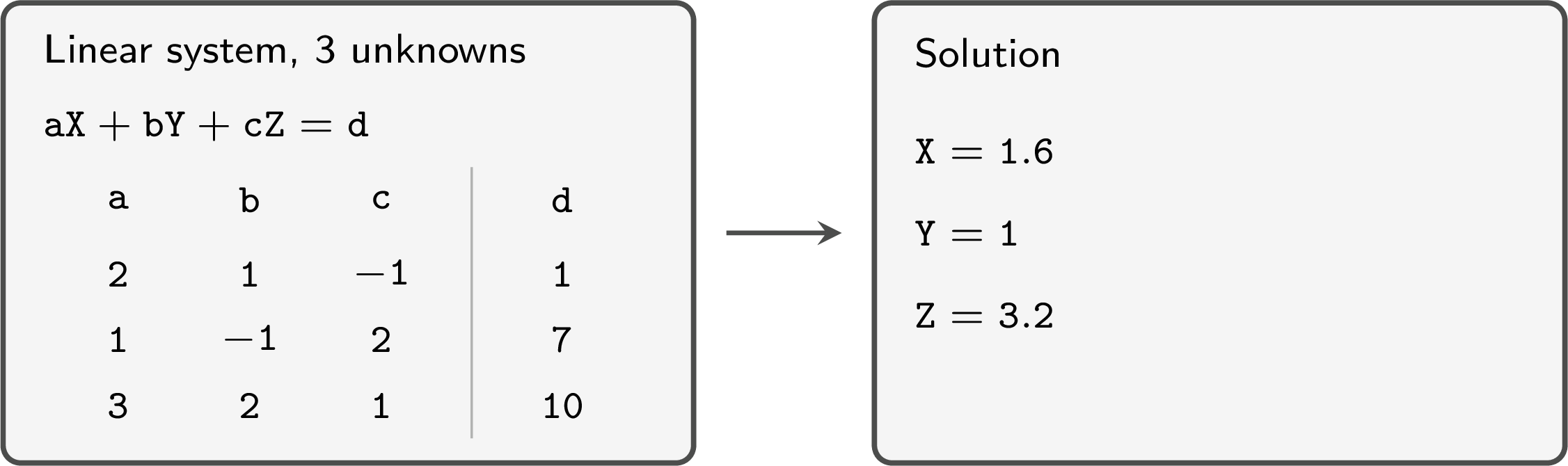
Method — Solving a Linear System with the Equation Solver
The linear system solver, in the equation menu of a graphing calculator, solves a system of two linear equations in two unknowns, or of three linear equations in three unknowns. - Write each equation in the form \(ax + by = c\) (two unknowns) or \(ax + by + cz = d\) (three unknowns): the unknowns on the left, in the same order in every equation, and the constant on the right.
- Open the linear system solver and choose the number of unknowns.
- Enter the coefficients row by row, one row per equation, each with its sign, and \(0\) for a missing unknown.
- Solve and read the value of each unknown. If the solver reports no solution, or infinitely many, the system has no unique solution.
- Check the solution by substituting it in each original equation, then report each value exactly when the checks hold exactly, otherwise to 3 significant figures.
Skills to practice
- The Linear System Solver
III.2
Three Equations with Technology
Example
Use technology to answer. - Solve the system \(\begin{cases} 0.6x + 1.5y = 4.2 \\ 2.4x - 0.9y = 1.5 \end{cases}\).
- The parabola \(y = ax^2 + bx + c\) passes through the points \(A(-1, 6)\), \(B(1, 2)\) and \(C(2, 3)\). Find \(a\), \(b\) and \(c\).
- Both equations already have the form \(ax + by = c\). The linear system solver, with two unknowns, the coefficients \(0.6\), \(1.5\), \(4.2\) in the first row and \(2.4\), \(-0.9\), \(1.5\) in the second, displays \(x = 1.4565217\) and \(y = 2.2173913\). Check in both equations with the displayed values; they are rounded, so the checks are approximate: $$0.6 \times 1.4565217 + 1.5 \times 2.2173913 \approx 4.2 \quad\text{and}\quad 2.4 \times 1.4565217 - 0.9 \times 2.2173913 \approx 1.5.$$ The solution is \(x \approx 1.46\) and \(y \approx 2.22\).
- Each point of the parabola gives an equation in \(a\), \(b\) and \(c\):
- \(A(-1, 6)\): \(a(-1)^2 + b(-1) + c = 6\), that is \(a - b + c = 6\);
- \(B(1, 2)\): \(a \times 1^2 + b \times 1 + c = 2\), that is \(a + b + c = 2\);
- \(C(2, 3)\): \(a \times 2^2 + b \times 2 + c = 3\), that is \(4a + 2b + c = 3\).
Skills to practice
- Solving Three Equations with the Solver
IV
Going further
Skills to practice
- Reasoning and Solving Problems
- Solving Problems with Technology
- Quiz
Jump to section