International Baccalaureate · DP 1: Applications and Interpretation HL
Bivariate Statistics
I
Measuring Correlation
I.1
Pearson's Correlation Coefficient
Recappreviously studied — click to reread
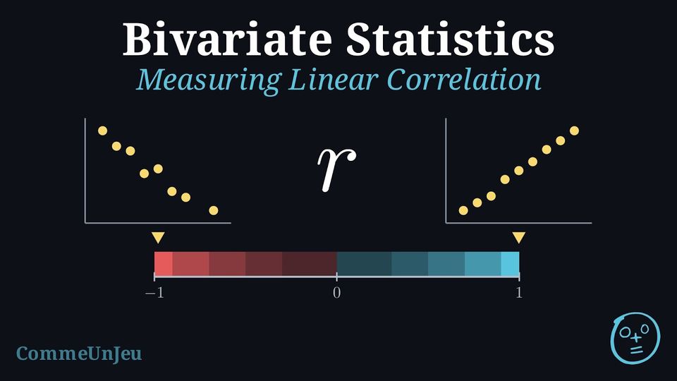
While scatter plots allow us to visually describe a correlation, this assessment is subjective. To provide a precise and objective measure of the strength and direction of a linear relationship, we use numerical coefficients.
Definition — Pearson's Correlation Coefficient (\(r\))
The Pearson's correlation coefficient (\(r\)) is a value in the range \([-1, 1]\) that quantifies the direction and strength of a linear relationship between two quantitative variables. - The sign of \(r\) indicates the direction (positive or negative).
- The magnitude (absolute value) of \(r\) indicates the strength. An \(|r|\) value close to 1 implies a strong linear correlation, while a value close to 0 implies a weak or no linear correlation.
| Value of \(|r|\) | Strength of Correlation |
| \(|r| = 1\) | Perfect |
| \(0.9 \le |r| < 1\) | Very Strong |
| \(0.7 \le |r| < 0.9\) | Strong |
| \(0.5 \le |r| < 0.7\) | Moderate |
| \(0.3 \le |r| < 0.5\) | Weak |
| \(0 \le |r| < 0.3\) | Very Weak or None |
Definition — Coefficient of Determination (\(r^2\))
The coefficient of determination (\(r^2\)) is the square of the correlation coefficient. It is a value in the range \([0, 1]\) and is typically expressed as a percentage.The value of \(r^2\) represents the proportion of the variance in the dependent variable (\(y\)) that is explained by the linear relationship with the independent variable (\(x\)). In simple terms, it tells us how well the linear model fits the data.
Example
A study of hours spent studying and exam scores finds a correlation coefficient of \(r = 0.9\).Interpret both \(r\) and \(r^2\).
- Interpretation of \(r\): Since \(r=0.9\), there is a very strong, positive, linear correlation between the hours spent studying and the exam scores.
- Interpretation of \(r^2\): We calculate \(r^2 = (0.9)^2 = 0.81\). This means that 81\(\pourcent\) of the variation in the exam scores can be explained by the linear relationship with the number of hours spent studying. The remaining 19\(\pourcent\) is not explained by the linear relationship.
Method — Obtaining \(r\) and \(r^2\) with Technology
In this method, the correlation coefficient \(r\) is not computed by hand: a calculator or a spreadsheet gives it from the data, together with \(r^2\). - Enter the data: the values of \(x\) in one list (or one column), the values of \(y\) in another, in the same order, so that each pair stays on the same row.
- Ask for the two-variable statistics: on a calculator, the two-variable statistics menu gives \(r\) and \(r^2\); on many models they appear on the linear regression screen \(y = ax + b\), beside the coefficients \(a\) and \(b\) of the least squares line (on some models, the display of \(r\) and \(r^2\) must first be switched on in the settings, and some models show only \(r\)); in a spreadsheet, with \(x\) in
A2:A9and \(y\) inB2:B9, the formula=CORREL(A2:A9,B2:B9)gives \(r\) and=RSQ(B2:B9,A2:A9)gives \(r^2\). - Round only at the end: keep the full value on the screen and give \(r\) and \(r^2\) rounded, usually to three decimal places; \(r^2\) is the square of the unrounded \(r\), so when only \(r\) is displayed, square the full value of \(r\).
- Check with the scatter plot: the sign of \(r\) should agree with the general direction of the cloud, and \(|r|\) with how closely the points follow a line. When they disagree, check that each pair was entered on the same row, and look for an outlier, which can change \(r\) a lot.
Example
The coach of a running club records, for eight runners, the distance \(x\) run in training each week, in kilometres, and the time \(y\) of each runner in a \(5\) km race, in minutes. | \(x\) (km) | \(10\) | \(15\) | \(20\) | \(25\) | \(30\) | \(35\) | \(40\) | \(50\) |
| \(y\) (min) | \(31.5\) | \(30.2\) | \(29.8\) | \(27.9\) | \(28.3\) | \(26.4\) | \(25.9\) | \(24.8\) |
- Use technology to find \(r\) and \(r^2\), rounded to three decimal places.
- Describe the correlation between \(x\) and \(y\).
- Interpret \(r^2\) in the context.
- With the distances in L1 and the times in L2, the linear regression gives the screen below.
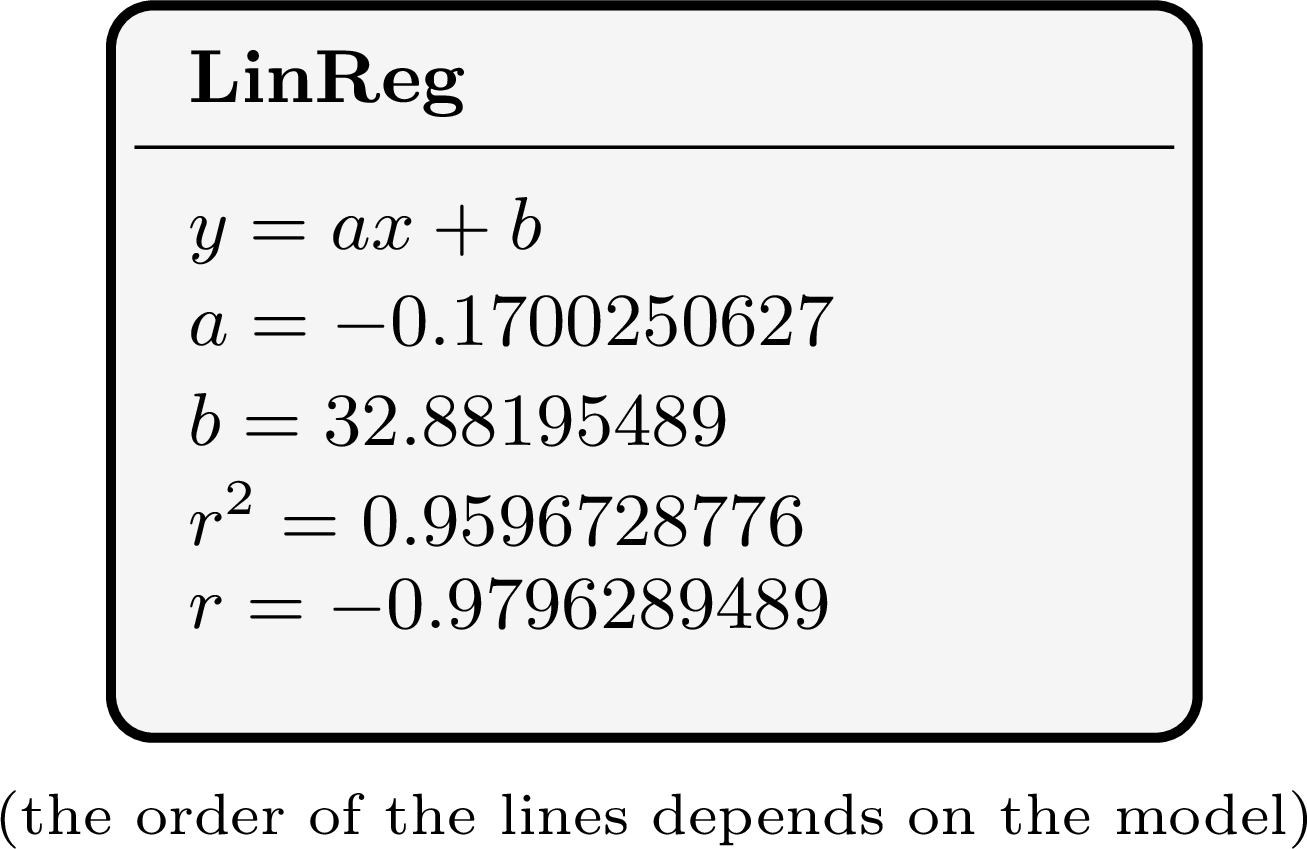
=CORREL(A2:A9,B2:B9)gives the same \(r\). - \(r\) is negative, so the correlation is negative: the runners who train more tend to have shorter race times. \(|r| \approx 0.980\) lies between \(0.9\) and \(1\), so the linear correlation is very strong. The sign agrees with the data: the times go down as the distances go up.
- \(r^2 \approx 0.960\): about \(96\pourcent\) of the variation in the race times is explained by the linear relationship with the training distance; the remaining \(4\pourcent\) is not explained by this linear relationship (other factors, measurement errors, natural variation). This is a correlation, not a proof that training alone makes the runners faster.
Skills to practice
- Computing the Correlation Coefficient with Technology
II
Lines of Best Fit
II.1
The Least Squares Regression Line
Recappreviously studied — click to reread
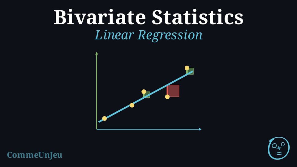
When a scatter plot indicates a linear correlation between two variables, we can model this relationship using a straight line. This line, known as the regression line, can be used to make predictions. How well the line fits the data is often summarised by the coefficient of determination (\(r^2\)). A high \(r^2\) value indicates that a large proportion of the variance in the dependent variable is explained by the linear relationship with the independent variable, suggesting the linear model is a good fit for the data, provided the scatter diagram shows no curve.
Definition — Least Squares Regression Line
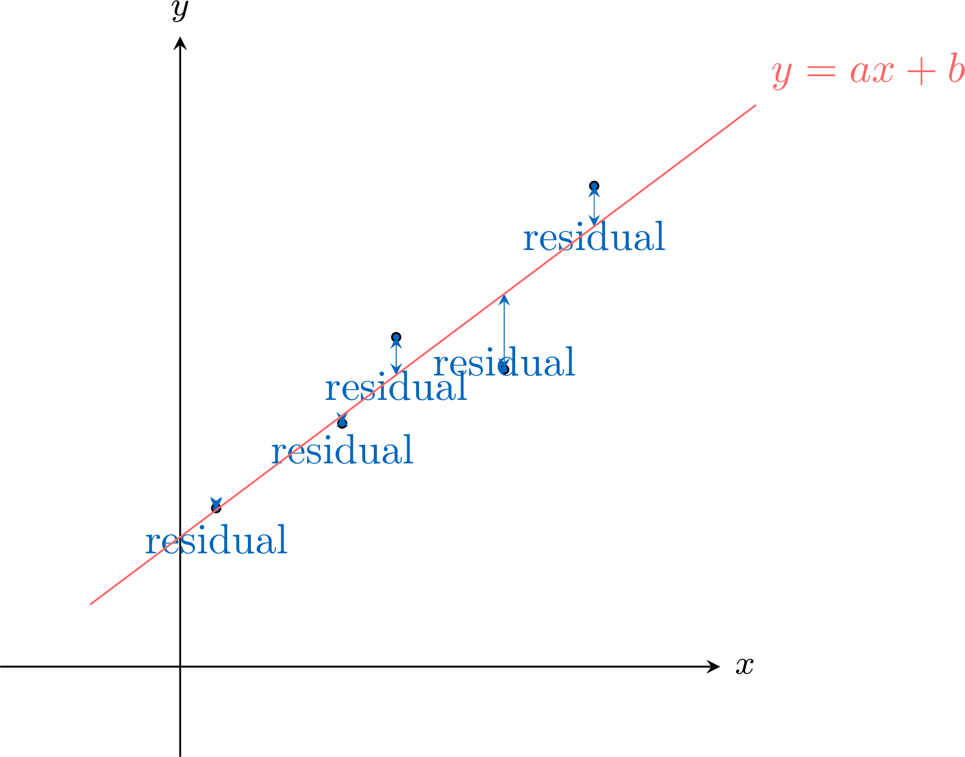
The least squares regression line, written as \(y = ax + b\), is the unique line of best fit (provided the \(x\)-values are not all equal) that models the linear relationship between \(x\) and \(y\). It is calculated by minimising the sum of the squares of the residuals.A residual is the signed vertical difference (positive above the line, negative below) between an observed data point \((x_i, y_i)\) and the predicted point on the regression line \((x_i, \hat{y}_i)\).$$ \text{Residual} = \text{observed } y - \text{predicted } y = y_i - \hat{y}_i $$ A key property is that the least squares regression line always passes through the mean point, \((\bar{x}, \bar{y})\).
Method — Obtaining the Least Squares Line with a Calculator or a Spreadsheet
The coefficients \(a\) and \(b\) of the least squares line \(y = ax + b\) are not computed by hand: a calculator or a spreadsheet gives them. - Enter the data: the values of \(x\) in one list (or one column), the values of \(y\) in another, in the same order.
- Ask for the line: on a calculator, the two-variable statistics menu, linear regression \(y = ax + b\); in a spreadsheet, with \(x\) in
A2:A6and \(y\) inB2:B6, the formulas=SLOPE(B2:B6,A2:A6)and=INTERCEPT(B2:B6,A2:A6), or a linear trend line added to the scatter plot, with its equation displayed. - Round sensibly: keep about as many significant figures as the measurements have, and write the equation with the letters of the situation.
- Check with the mean point: the least squares line passes through \(G(\bar{x}, \bar{y})\); replacing \(x\) by \(\bar{x}\) in the equation must give \(\bar{y}\), up to rounding.
Example
A laboratory prepares five solutions of known concentration \(x\), in milligrams per litre, and measures the absorbance \(y\) of each one. | \(x\) | \(2\) | \(4\) | \(6\) | \(8\) | \(10\) |
| \(y\) | \(0.11\) | \(0.19\) | \(0.31\) | \(0.40\) | \(0.49\) |
- Give, with a calculator, the equation of the least squares line, with \(a\) rounded to four decimal places and \(b\) to three.
- Check that this line passes through the mean point.
- Predict the absorbance of a solution of concentration \(7\) mg/L.
- A sample of unknown concentration has an absorbance of \(0.35\). Explain why, in general, a regression line of \(y\) on \(x\) should not be used to estimate \(x\) from a measured value of \(y\). Then explain why this calibration line may nevertheless be solved for \(x\), and estimate the concentration of the sample.
- The calculator gives \(a = 0.0485\) and \(b = 0.009\): the calibration line is \(y = 0.0485x + 0.009\) (the gradient is kept with three significant figures).
- \(\bar{x} = 6\) and \(\bar{y} = 0.30\). For \(x = 6\) the equation gives \(0.0485 \times 6 + 0.009 = 0.300\): the line passes through \(G(6, 0.30)\).
- \(0.0485 \times 7 + 0.009 = 0.3485\): the expected absorbance is about \(0.35\).
- The line of \(y\) on \(x\) makes the sum of the squares of the vertical distances between the points and the line as small as possible: it is built to estimate \(y\) from \(x\). Estimating \(x\) from \(y\) would require the horizontal distances to be small, and solving \(y = 0.0485x + 0.009\) for \(x\) does not give the line that achieves this: when both variables vary from one individual to another, the line of \(y\) on \(x\) is not used to estimate \(x\). Here the situation is different: the laboratory chose the concentrations in advance, and only the absorbance is measured. The value of \(x\) is fixed and only \(y\) varies from one measurement to the next, so the model is the line of \(y\) on \(x\), and the usual practice with a calibration line is to solve it for \(x\). Solve \(0.0485x + 0.009 = 0.35\): \(x = \dfrac{0.35 - 0.009}{0.0485} \approx 7.0\). The concentration is about \(7.0\) mg/L. This value lies between \(2\) and \(10\) mg/L, the smallest and the largest concentrations measured: the line is used inside the range where it was fitted.
Definition — Interpolation and Extrapolation
The line of best fit can be used to make predictions: - Interpolation is the process of predicting a \(y\)-value for an \(x\)-value that is within the range of the original data. If the correlation is strong, interpolation is generally considered reliable (provided the linear model fits the data well).
- Extrapolation is the process of predicting a \(y\)-value for an \(x\)-value that is outside the range of the original data. Extrapolation is generally considered unreliable, as we cannot assume the linear trend continues indefinitely.
Example
For a survey of hours studied and exam scores (out of \(100\)), a calculator gives the line of best fit \(y = 3.5x + 40\). In this dataset, the hours studied ranged from 2 to 15. - Predict the exam score for a student who studied for 11 hours.
- Predict the exam score for a student who studied for 25 hours.
- Comment on the reliability of the prediction in question 2.
- Since \(x=11\) is within the data range, this is interpolation. $$ y = 3.5(11) + 40 = 38.5 + 40 = 78.5 $$ The predicted score is 78.5.
- Since \(x=25\) is outside the data range, this is extrapolation. $$ y = 3.5(25) + 40 = 87.5 + 40 = 127.5 $$ The predicted score is 127.5.
- The prediction in question 2 is unreliable. It is an extrapolation, and we cannot assume the linear relationship holds for 25 hours of study. Furthermore, the model predicts a score over 100, which is impossible in this context, highlighting the danger of extrapolation.
Skills to practice
- Fitting a Line in Context with a Calculator
III
Reliability and Validity
III.1
Reliability and Validity Tests
Judging a Measuring Instrument
A bathroom scale, a questionnaire, a reading test or a step counter is an instrument: it turns each individual into a number. Before trusting the data it produces, two questions are asked. Does it give the same result when the measurement is repeated? Does it measure what it claims to measure? The first question is about reliability, the second about validity, and the correlation coefficient \(r\) answers part of both.
Definition — Reliability
A measurement is reliable when it measures consistently: repeated on the same individuals, under the same conditions, it gives similar results. Two tests of reliability are used. - Test-retest reliability: the same test is given twice to the same individuals, under the same conditions, some time apart; the two sets of results are compared. Its weakness: between the two occasions, the individuals may remember the answers, learn, or change.
- Parallel forms reliability: two versions of the test, built to be equivalent (same content, same difficulty), are given to the same individuals; the results of the two versions are compared. Its weakness: the two versions must really be equivalent.
Definition — Validity
A measurement is valid when it measures accurately what it is intended to measure. Two kinds of validity are distinguished. - Content validity: the instrument covers, in a representative way, the field it claims to assess (its topics and its skills, at suitable levels of difficulty). It is judged with a knowledge of that field, not by a calculation.
- Criterion-related validity: the measurement agrees with an established and trusted measurement of the same thing, or predicts a later outcome that it is meant to predict; this reference is called the criterion variable. It is judged by the strength of the correlation between the measurement and the criterion variable: the closer \(|r|\) is to \(1\), with the sign expected from the way the two variables are scored, the stronger the evidence of validity. A strong correlation shows agreement in order and in trend; to check that the values themselves agree, the differences between the measurement and the criterion are also examined.
Method — Assessing Reliability and Validity with a Correlation Coefficient
- Identify the comparison: the same test twice (test-retest reliability), two equivalent versions (parallel forms reliability), or the measurement against a criterion variable (criterion-related validity).
- Pair the results individual by individual, and calculate \(r\) with technology.
- Judge: reliability requires a strong positive correlation, \(r\) close to \(1\), with paired values close to each other; for criterion-related validity, the closer \(|r|\) is to \(1\), the stronger the evidence. The sign then depends on how the two variables are scored: a ranking where \(1\) is the best, compared with a score where more is better, gives a negative \(r\).
- Know the limits: a strong correlation shows that the results agree in order and in trend, not that they are equal. An instrument can be reliable without being valid: a scale that always shows \(2\) kg too much is perfectly consistent, and the correlation between its readings and the true masses is \(1\). Content validity is judged, never calculated.
Example
A coach measures the standing long jump, in centimetres, of ten athletes on a Monday, then again on the Thursday of the same week, under the same conditions. | athlete | \(1\) | \(2\) | \(3\) | \(4\) | \(5\) | \(6\) | \(7\) | \(8\) | \(9\) | \(10\) |
| Monday | \(182\) | \(205\) | \(168\) | \(221\) | \(194\) | \(176\) | \(210\) | \(188\) | \(199\) | \(215\) |
| Thursday | \(185\) | \(201\) | \(172\) | \(224\) | \(190\) | \(180\) | \(212\) | \(185\) | \(203\) | \(218\) |
- Which type of reliability is being considered?
- Use technology to find the correlation coefficient \(r\) between the two sets of jumps.
- Comment on the reliability of the standing long jump as a measurement.
- The coach wants to use this single jump to measure the overall physical fitness of the athletes. Comment on the content validity of this choice.
- The same test is repeated on the same athletes, under the same conditions, three days apart: this is test-retest reliability.
- With the Monday jumps in L1 and the Thursday jumps in L2, the calculator gives \(r = 0.9805\ldots\), so \(r \approx 0.981\).
- \(r \approx 0.981\) is positive and very close to \(1\): the athletes who jump far on Monday also jump far on Thursday, and the changes from one day to the other are small (at most \(4\) cm). Over a few days, for this group, the standing long jump is a reliable measurement.
- Reliability does not make it valid for this purpose. Overall fitness includes endurance, strength of the whole body, speed and flexibility; one jump measures mainly the power of the legs. The content validity of this choice is low: a valid fitness test would combine several exercises that cover the whole field.
Example
To check a new step-counting app, eight walks are filmed and the steps are counted by hand, one by one, which gives the true number of steps. The app counts the same walks. | by hand | \(1200\) | \(2500\) | \(3100\) | \(4000\) | \(4800\) | \(5600\) | \(6300\) | \(7500\) |
| app | \(1270\) | \(2610\) | \(3270\) | \(4210\) | \(5040\) | \(5880\) | \(6630\) | \(7870\) |
- Which type of validity is being checked? What is the criterion variable?
- Use technology to find \(r\) between the counts by hand and the counts of the app.
- Does this value show that the app counts the steps accurately?
- The app is compared with an established and trusted measurement of the same thing: this is criterion-related validity, and the criterion variable is the number of steps counted by hand.
- With the counts by hand in L1 and the app counts in L2, the calculator gives \(r = 0.99998\ldots\), so \(r \approx 1.000\).
- No. The correlation is almost perfect, so the app ranks the walks in the right order and its counts follow the true ones very closely along a line. But it counts too many steps on every walk: \(70\) too many on the shortest walk, \(370\) on the longest, about \(5\pourcent\) each time (for instance \(\frac{7870}{7500} \approx 1.049\)). This systematic error is invisible to \(r\). The app agrees very well with the criterion in trend, but its counts are about \(5\pourcent\) too high: to judge accuracy, the values themselves must be compared.
Skills to practice
- Identifying Reliability and Validity Tests
- Calculating a Reliability or Validity Coefficient
- Judging Reliability and Validity
IV
Spearman's Rank Correlation
IV.1
Spearman's Rank Correlation Coefficient
When the Trend Is Not a Line
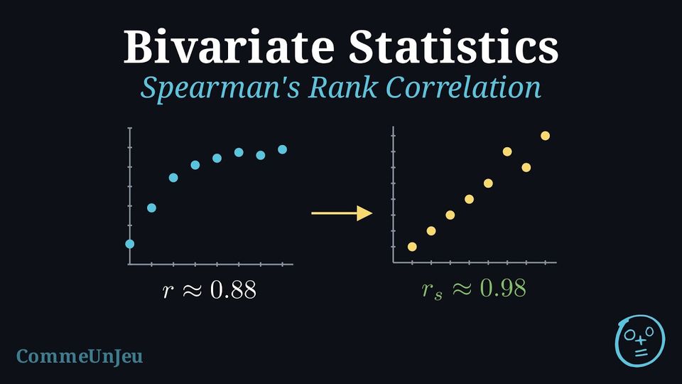
Pearson's coefficient \(r\) measures how closely the points of a scatter diagram follow a line. Many relationships go steadily up, or steadily down, without following a line: a plant grows quickly and then more and more slowly; a medicine leaves the blood quickly and then slowly. For such data, \(r\) underestimates how regular the relationship is. Spearman's idea is to forget the values and to keep only their order: which value is the smallest, which is the second smallest, and so on.
Definition — Ranks and Ties
To rank a list of \(n\) values, order them from the smallest to the largest: the smallest value has rank \(1\), the next one rank \(2\), and so on up to rank \(n\). Equal values are called ties; each of them receives the mean of the ranks that they occupy together.For instance, in the list \(12, 15, 15, 18\), the two values \(15\) occupy the ranks \(2\) and \(3\), so each receives the rank \(\frac{2 + 3}{2} = 2.5\): the ranks are \(1, 2.5, 2.5, 4\).
Definition — Spearman's Rank Correlation Coefficient
Let \((x_1, y_1), (x_2, y_2), \ldots, (x_n, y_n)\) be bivariate data. Rank the \(x\)-values among themselves, and the \(y\)-values among themselves (neither variable being constant). Spearman's rank correlation coefficient, written \(r_s\), is Pearson's correlation coefficient of the ranks: each pair \((x_i, y_i)\) is replaced by the pair (rank of \(x_i\), rank of \(y_i\)), and \(r\) is calculated for these new pairs.A relationship between \(x\) and \(y\) is monotonic when, as \(x\) increases, \(y\) never goes down (an increasing relationship), or never goes up (a decreasing relationship). To tell the two coefficients apart, Pearson's coefficient is sometimes written \(r_p\).
Proposition — Reading Spearman's Coefficient
- Like any Pearson coefficient, \(-1 \le r_s \le 1\).
- For data without ties, \(r_s = 1\) exactly when the ranks of \(y\) are the ranks of \(x\), that is when \(y\) increases every time \(x\) increases; \(r_s = -1\) exactly when \(y\) decreases every time \(x\) increases.
- The sign of \(r_s\) gives the direction of the trend (increasing or decreasing), and \(|r_s|\) close to \(1\) means a strong monotonic relationship. The scale of strength used for \(r\) is used for \(r_s\) in the same way.
- \(r_s\) says nothing about linearity: \(r_s = 1\) for points that rise along a curve.
Proposition — Spearman's Formula without Ties
When no two \(x\)-values are equal and no two \(y\)-values are equal, $$r_s = 1 - \frac{6\sum d^2}{n(n^2 - 1)},$$ where \(n\) is the number of pairs and \(d\) is, for each pair, the difference between the rank of \(x\) and the rank of \(y\). When there are ties, this formula is no longer valid in general, and its error can be large: \(r_s\) is then calculated as Pearson's coefficient of the ranks, with technology. Method — Calculating Spearman's Coefficient
- Rank each variable separately: the \(x\)-values among themselves, the \(y\)-values among themselves, from the smallest (rank \(1\)), giving tied values the mean of their ranks.
- With technology: enter the ranks of \(x\) and the ranks of \(y\) in two lists and ask for \(r\), as for any bivariate data: the value displayed is \(r_s\). In a spreadsheet,
=RANK.AVG(A2,A2:A9,1)gives the rank of the value inA2among the values ofA2:A9, ties averaged (fix the range before copying the formula down);=CORRELapplied to the two columns of ranks then gives \(r_s\). Some calculators and software give \(r_s\) directly. - By hand, when there are no ties: write the difference \(d\) of the two ranks for each pair, then \(\sum d^2\), and apply Spearman's formula.
- Interpret: state the direction and the strength of the monotonic trend, in the words of the context.
Example
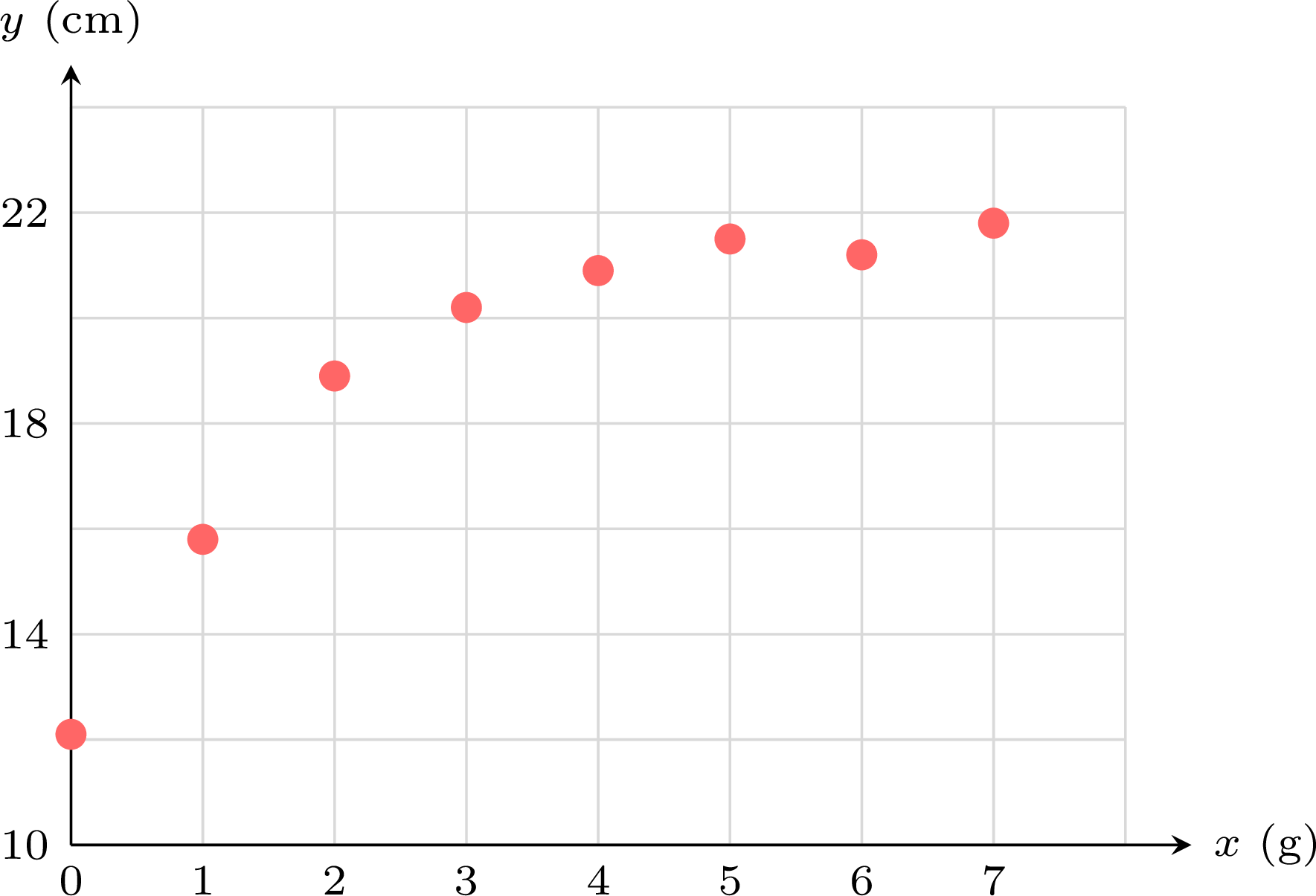
Eight identical seedlings receive different amounts \(x\) of fertiliser, in grams; their height \(y\), in centimetres, is measured four weeks later. | \(x\) (g) | \(0\) | \(1\) | \(2\) | \(3\) | \(4\) | \(5\) | \(6\) | \(7\) |
| \(y\) (cm) | \(12.1\) | \(15.8\) | \(18.9\) | \(20.2\) | \(20.9\) | \(21.5\) | \(21.2\) | \(21.8\) |
- Draw the scatter diagram and use technology to find Pearson's coefficient \(r\).
- Rank each variable and calculate Spearman's coefficient \(r_s\).
- Which coefficient describes this relationship better? Describe the correlation.
- The points rise quickly, then flatten out:
- The values of \(x\) are already in increasing order, so their ranks are \(1\) to \(8\). The heights ordered from the smallest are \(12.1, 15.8, 18.9, 20.2, 20.9, 21.2, 21.5, 21.8\), so \(21.2\) has rank \(6\) and \(21.5\) rank \(7\):
rank of \(x\) \(1\) \(2\) \(3\) \(4\) \(5\) \(6\) \(7\) \(8\) rank of \(y\) \(1\) \(2\) \(3\) \(4\) \(5\) \(7\) \(6\) \(8\) \(d\) \(0\) \(0\) \(0\) \(0\) \(0\) \(-1\) \(1\) \(0\) - The height rises quickly for the first grams of fertiliser, then much more slowly from \(3\) g on, with even a slight drop between \(5\) g and \(6\) g: the cloud bends, it does not follow a line. Apart from this one pair, the order of the heights is the order of the doses, which \(r_s \approx 0.976\) expresses, while \(r \approx 0.882\) is lower, mainly because the points are not on a line. Spearman's coefficient is the appropriate one: there is a very strong increasing trend between the amount of fertiliser and the height, and it is not linear.
Method — Choosing between \(r\) and \(r_s\)
- Look at the scatter diagram first: a coefficient summarises a cloud, it never replaces it.
- Points close to a line: Pearson's \(r\) measures the strength of the linear relationship; it is the coefficient that goes with the least squares line.
- Points rising or falling steadily along a curve, or data that are ranks (positions in a competition, preferences, marks given by judges): Spearman's \(r_s\) measures the strength of the monotonic relationship.
- Beware of outliers: a single point far from the others can create or hide a linear correlation, so \(r\) is very sensitive to outliers. In the ranks, however far a point is, its rank is at most \(n\) or at least \(1\): its influence is bounded, so \(r_s\) is usually less sensitive, although moving one point can still shift several ranks. An outlier is not removed because it is far: only when it is an error, or when it does not belong to the population studied.
- Points that rise and then fall (or the reverse): neither coefficient describes the turning point; when the rise and the fall balance, both can be close to \(0\) while the points follow a clear pattern. Describe the shape of the cloud instead.
Example
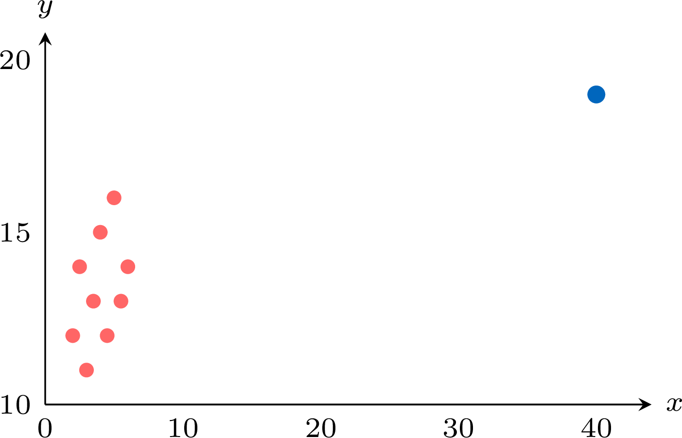
Ten pupils note the number of hours \(x\) that they revised during the week before a test, and their mark \(y\) out of \(20\). | \(x\) | \(2\) | \(2.5\) | \(3\) | \(3.5\) | \(4\) | \(4.5\) | \(5\) | \(5.5\) | \(6\) | \(40\) |
| \(y\) | \(12\) | \(14\) | \(11\) | \(13\) | \(15\) | \(12\) | \(16\) | \(13\) | \(14\) | \(19\) |
- Rank the marks.
- Use technology to find \(r\) and \(r_s\).
- The value \(40\) hours is a recording error, and the true value is unknown. Remove this pupil, then find \(r\) and \(r_s\) again.
- Which coefficient did the error change more? Explain why.
- Ordered, the marks are \(11, 12, 12, 13, 13, 14, 14, 15, 16, 19\). The two \(12\)s share the ranks \(2\) and \(3\), so each has rank \(2.5\); likewise the \(13\)s have rank \(4.5\) and the \(14\)s rank \(6.5\):
\(y\) \(12\) \(14\) \(11\) \(13\) \(15\) \(12\) \(16\) \(13\) \(14\) \(19\) rank \(2.5\) \(6.5\) \(1\) \(4.5\) \(8\) \(2.5\) \(9\) \(4.5\) \(6.5\) \(10\) - The linear regression on \(x\) and \(y\) gives \(r = 0.7929\ldots \approx 0.793\). The values of \(x\) are all different and already in increasing order, so their ranks are \(1\) to \(10\); Pearson's coefficient of the ranks of \(x\) and the ranks of \(y\) gives \(r_s = 0.5688\ldots \approx 0.569\). There are ties, so Spearman's formula is not exact here.
- Without the tenth pupil, technology gives \(r = 0.4041\ldots \approx 0.404\) and \(r_s = 0.4050\ldots \approx 0.405\).
- The error moved \(r\) from \(0.404\) to \(0.793\): this single point almost doubled \(r\) and suggested a strong linear correlation that the other nine pupils do not show. It moved \(r_s\) from \(0.405\) to \(0.569\), much less. In the values, the point \((40, 19)\) lies \(34\) hours beyond all the others:
Skills to practice
- Choosing a Correlation Coefficient
- Calculating Spearman's Coefficient
- Comparing Pearson's and Spearman's Coefficients in Context
V
Going further
Skills to practice
- Analysing Bivariate Data with Technology
- Reasoning about Correlation and Regression
- Solving Problems on Rank Correlation and Reliability
- Quiz
Jump to section