International Baccalaureate · DP 1: Applications and Interpretation HL

Modelling

⌚ ~122 min ▢ 13 blocks ✓ 49 exercises ➣ Prerequisites : Straight Lines, Quadratic Functions, Functions

I The Modelling Cycle

Recappreviously studied — click to reread

Mathematical modelling is the process of using mathematics to represent, analyse, and predict real-world phenomena. A model typically links measurable variables through a function whose parameters are chosen from data or from reasonable assumptions. From the trajectory of a ball to changes in stock prices, functions provide a precise framework for describing patterns and making informed predictions.

Report an error

Definition — Mathematical Model

A mathematical model is a function (or system of equations) that represents the relationship between variables in a real-world situation.

The variables represent quantities that can change (e.g., time, height, cost).
The parameters are constants chosen to fit a context or a data set.
The model is only intended to be used on a stated domain where it is meaningful.

Method — 5 Steps of Modelling

You should follow these steps:

Construct: Create a model from data or from a verbal description. This includes choosing a suitable functional form (linear, quadratic, etc.) and determining its parameters.
Use: Use the model to make predictions.
- Interpolation: Predict within the range of the available data.
- Extrapolation: Predict outside the range of the data (often less reliable).
Interpret: Explain the meaning of variables and parameters in context (e.g., what does the $y$-intercept represent?).
Evaluate: Assess the validity of the model: compare with data, compute errors, analyse residuals/correlation (if relevant), and check whether the results are realistic.
Refine: Suggest improvements if the model is inadequate (e.g., “an exponential model grows too fast; a logistic model may be more appropriate”).

Skills to practice

Identifying Variables and Parameters

II Linear Models

Recappreviously studied — click to reread

Linear models are the simplest functional models. They describe situations where a quantity changes at a constant rate with respect to another variable. Common applications include cost functions (fixed fee plus hourly rate), distance travelled at constant speed, and currency conversions.

Report an error

Definition — Linear Model

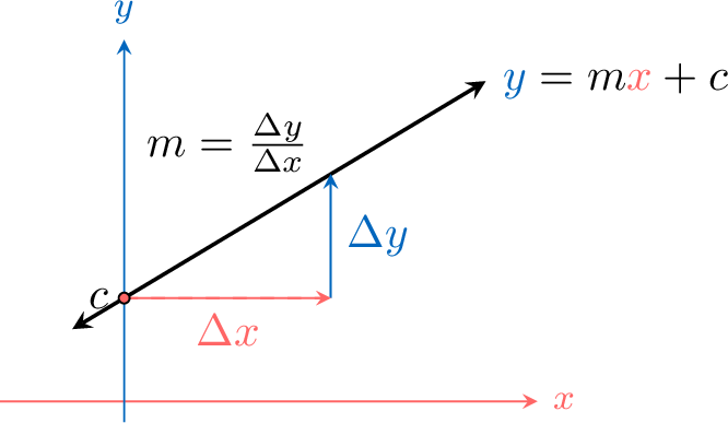
A linear model relates two variables with a constant rate of change:$$ f(x) = mx + c. $$

$m$: the gradient (rate of change).
$c$: the $y$-intercept (initial value), i.e. $f(0)=c$.

Example

A plumber charges a fixed call-out fee of $\dollar$50 plus $\dollar$80 per hour of work.
The cost model is $C(t) = 80t + 50$, where $t$ is the time in hours.

Calculate the cost for 10 hours.
Find the time for the total cost to exceed $\dollar$1200.
Under a new tax, the plumber changes the hourly rate to $\dollar$80 and the fixed fee to $\dollar$100. Write the new cost function after these changes have been made.

Answer

Cost for 10 hours: $$ C(10) = 80(10) + 50 = 800 + 50 = 850. $$ The cost is $\dollar$850.
Time to exceed $\dollar$1200: $$ 80t + 50 > 1200 \implies 80t > 1150 \implies t > \frac{1150}{80} = 14.375. $$ So the cost exceeds $\dollar$1200 after $14.375$ hours (i.e.\ 14 hours 22 minutes 30 seconds).
New cost function: The new hourly rate is $\dollar$80 and the new fixed fee is $\dollar$100: $$ C_{\text{new}}(t) = 80t + 100. $$

Skills to practice

Linear Models

III Building Linear Models from Data

Example

An electric scooter shows a charge of $15\pourcent$ when it is plugged in, and a charge of $39\pourcent$ twenty minutes later. Its owner wants to know when the battery will be fully charged.

Construct a linear model for the charge $C$, in percent, $t$ minutes after the scooter is plugged in. State the assumption made.
Interpret the two parameters of the model.
Use the model to predict when the battery is fully charged, and state a domain for the model.
The battery actually reaches $100\pourcent$ after $85$ minutes. Test the model against this value, reflect on it, and suggest a refinement.

Answer

Construct. Assumption: the battery charges at a constant rate, that is, it gains the same charge every minute. Under this assumption the graph of $C$ against $t$ is the line through the two readings $(0, 15)$ and $(20, 39)$. Its gradient is $$\begin{aligned}[t] m &= \frac{39 - 15}{20 - 0} && \text{(gradient between the two readings)}\\ &= 1.2, \end{aligned}$$ and its $C$-intercept is the charge at $t = 0$, that is $15$. The model is $C(t) = 1.2t + 15$.
Interpret. $15 = C(0)$ is the charge, in percent, when the scooter is plugged in; $1.2$ is the charge gained each minute, in percentage points per minute.
Use. The battery is full when $C(t) = 100$: $$\begin{aligned}[t] 1.2t + 15 &= 100 \\ 1.2t &= 85 && \text{(subtract } 15\text{)}\\ t &= \frac{85}{1.2} \approx 70.8. && \text{(divide by } 1.2\text{)} \end{aligned}$$ The model predicts a full charge after about $71$ minutes. A charge cannot exceed $100\pourcent$, so the model is used on the domain $0 \le t \le \frac{85}{1.2}$, that is from $0$ to about $70.8$ minutes.
Test. The model predicts $70.8$ minutes and the battery takes $85$: the model underestimates the charging time by about $14$ minutes, that is about $17\pourcent$ of the actual time.
Reflect. The model fits the two readings it was built from, so the error comes from the way it was built: two readings only, and the assumption of a constant rate. The most likely cause is that the charge does not rise at a constant rate: like most batteries, this one probably charges more slowly when it is nearly full. Readings taken during the charge, and near its end, would test this explanation. The model is useful to predict the charge during the first part of the charging, not the time of a full charge.
Refine. Assume that the rate stays $1.2$ up to $80\pourcent$, which the model reaches at $t = \frac{65}{1.2} \approx 54.2$ minutes. The last $20$ percentage points then take $85 - \frac{65}{1.2} \approx 30.8$ minutes, a rate of $\frac{20}{85 - 65/1.2} \approx 0.649$ percentage points per minute. The refined model is a piecewise linear model with two pieces; it must in turn be tested against new readings.

Skills to practice

Building and Using Linear Models
Applying Linear Models

IV Piecewise Linear Models

Piecewise linear models are used when the rate of change of a function differs across intervals. These commonly apply to tariffs, tax brackets, or physical motion.

Report an error

Definition — Piecewise Linear Model

A piecewise linear model is defined by different linear rules on different parts of the domain:$$ f(x) = \begin{cases}m_1x + c_1 & \text{if } x \le a,\\ m_2x + c_2 & \text{if } x > a.\end{cases} $$

The model may be continuous or discontinuous at the change point $x=a$.
If it is continuous and the gradient changes, the graph has a “corner” (a kink) at $x=a$.

Example

The total monthly charge, $\dollar C$, of a phone bill can be modelled by the function:$$C(m) = \begin{cases}10 + 0.02m & 0 \leq m \leq 100 \\ 9 + 0.03m & m > 100\end{cases}$$ where $m$ is the number of minutes used.

Find the total monthly charge if 80 minutes have been used.
Given that the total monthly charge is $\dollar$16.59, find the number of minutes that were used.

Answer

Calculate cost for $m=80$: Since $80 \le 100$, use the first rule: $$ C(80) = 10 + 0.02(80) = 10 + 1.60 = 11.60\dollar. $$
Calculate minutes for $C=16.59$: First compute the cost at the end of the first interval: $$ C(100) = 10 + 0.02(100) = 12. $$ Since $16.59 > 12$, we must have $m>100$, so use the second rule: $$\begin{aligned} 16.59 &= 9 + 0.03m \\ 7.59 &= 0.03m \\ m &= \frac{7.59}{0.03}\\ m&= 253. \end{aligned} $$ Therefore, $m=253$ minutes.

Example

A print shop charges for flyers according to the piecewise linear model shown below, for orders of up to $500$ flyers, where $C$ is the cost in dollars and $n$ the number of flyers.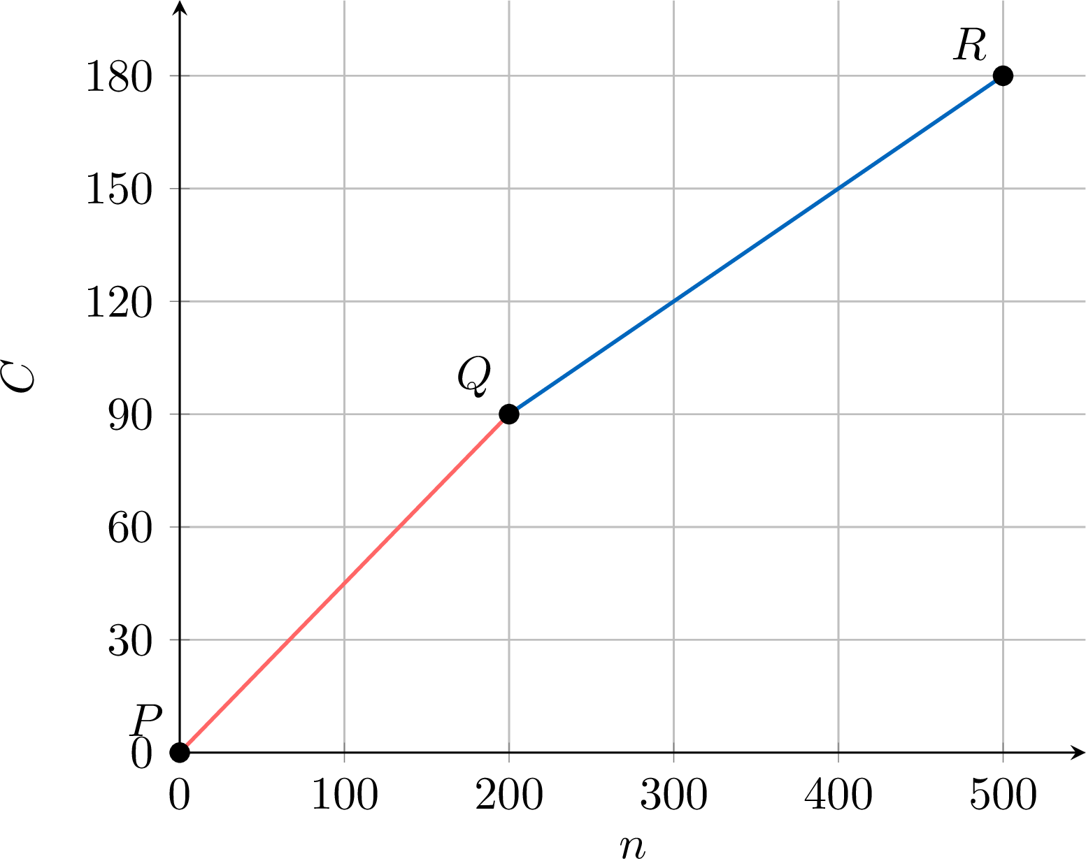

Find the gradient of the segment $\Segment{PQ}$ and of the segment $\Segment{QR}$. Interpret each gradient.
Find the cost of printing $120$ flyers.
Find the number of flyers that can be printed for $\dollar 132$.
Write the model as a piecewise function of the number of flyers.

Answer

The graph gives $P(0, 0)$, $Q(200, 90)$ and $R(500, 180)$. $$\begin{aligned}[t] \text{gradient of } \Segment{PQ} &= \frac{90 - 0}{200 - 0} = 0.45, \\ \text{gradient of } \Segment{QR} &= \frac{180 - 90}{500 - 200} = \frac{90}{300} = 0.3. \end{aligned}$$ Each of the first $200$ flyers costs $\dollar 0.45$; each flyer after the first $200$ costs $\dollar 0.30$. A gradient of a cost model is a price per unit.
$120 \le 200$, so the point lies on $\Segment{PQ}$: $C = 0.45 \times 120 = 54$. Printing $120$ flyers costs $\dollar 54$.
The cost of $200$ flyers is $\dollar 90 < \dollar 132$, so the order has more than $200$ flyers and the point lies on $\Segment{QR}$: the cost is $90$ plus $0.3$ per flyer after the first $200$. $$\begin{aligned}[t] 90 + 0.3(n - 200) &= 132 \\ 0.3(n - 200) &= 42 && \text{(subtract } 90\text{)}\\ n - 200 &= 140 && \text{(divide by } 0.3\text{)}\\ n &= 340. \end{aligned}$$ Check: $90 + 0.3 \times 140 = 132$. $\dollar 132$ pays for $340$ flyers.
$$C(n) = \begin{cases} 0.45n & \text{if } 0 \le n \le 200,\\ 90 + 0.3(n - 200) & \text{if } 200 < n \le 500. \end{cases}$$ Here $n$ is a whole number of flyers; the graph joins the costs by segments. The second piece simplifies to $0.3n + 30$. Both pieces give $90$ at $n = 200$: the graph has no jump there, and it has a kink at $Q$, where the gradient changes.

Skills to practice

Using Piecewise Linear Models
Applying Piecewise Linear Models

V Cubic Models

Definition — Cubic Model

A cubic model is a function of the form$$ f(x)=ax^3+bx^2+cx+d, \qquad a\neq 0. $$

$a$ determines the overall end behaviour of the graph and its vertical stretch.
$d$ is the $y$-intercept, since $f(0)=d$.

Example

The vertical height of a child above the ground, $h$ metres, as they go down a water slide can be modelled by the function$$h(t) = \frac{4}{7}(35 - 12t + 6t^2 - t^3),$$ where $t$ is the time in seconds after the child enters the slide.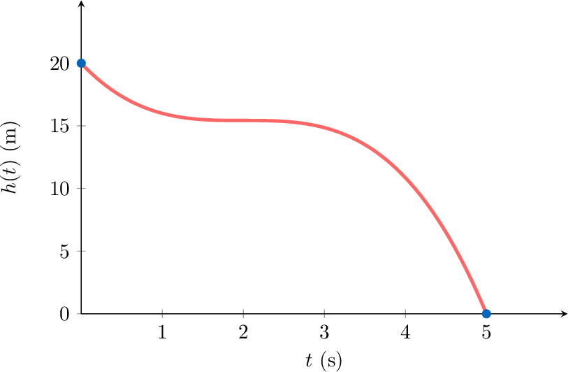

State the vertical height of the slide.
Given that the child reaches the ground at the bottom of the slide, find the domain of the function.

Answer

The height of the slide is the initial height at $t=0$.$$ h(0) = \frac{4}{7}(35) = 20 \text{ m}. $$
The child reaches the ground when $h(t) = 0$.$$ \frac{4}{7}(35 - 12t + 6t^2 - t^3) = 0 \implies 35 - 12t + 6t^2 - t^3 = 0. $$ Using a calculator or inspection, $t=5$ is a root:$$ 35 - 12(5) + 6(25) - 125 = 35 - 60 + 150 - 125 = 0. $$ Since the child starts at $t=0$ and reaches the ground at $t=5$, the physically meaningful domain is $0 \le t \le 5$.

Skills to practice

Applying Cubic Models

VI Direct and Inverse Variation

Recappreviously studied — click to reread

Variation models describe how one quantity changes in relation to another. They are fundamental in physics and geometry.

Report an error

Definition — Direct Variation

Two variables are said to vary directly if one is a constant multiple of the other.$$ y = kx, \qquad k \text{ constant}. $$ Equivalently, for $x\neq 0$, the ratio $\frac{y}{x}$ is constant.

Example

If $ y $ and $ x^n $ (for a positive integer $ n $) vary directly, then:
- It is denoted as $ y \propto x^n $
- $ y = kx^n $ for some constant $ k $
- This can be written as $ \frac{y}{x^n} = k $ (for $x\neq 0$)
For $n \ge 1$, the graph of $y=kx^n$ passes through the origin $(0,0)$.

Method — Find the equation of a direct variation model

Identify which two variables vary directly (e.g., $y$ and $x^2$).
Write the generic equation: $y = kx^n$.
Use a given pair $(x,y)$ to find the constant $k$.
Write the specific equation.
Use the equation to solve problems.

Example

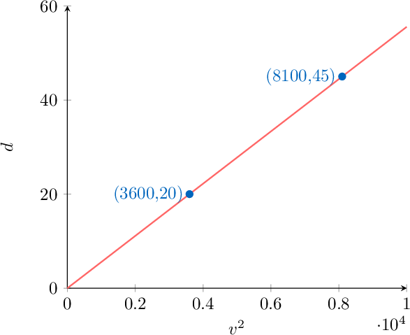
The braking distance, $d$ metres, of a car varies directly with the square of its speed, $v$ km/h. A car travelling at 60 km/h has a braking distance of 20 metres.

Find an equation connecting $d$ and $v$.
Find the braking distance for a car travelling at 90 km/h.

Answer

Equation: We are told $d \propto v^2$, so $d = kv^2$. Using $d=20$ when $v=60$: $$ 20 = k(60)^2 \implies 20 = 3600k \implies k = \frac{20}{3600} = \frac{1}{180}. $$ Hence $d = \frac{1}{180}v^2$.
Prediction: When $v=90$: $$ d = \frac{1}{180}(90)^2 = \frac{8100}{180} = 45 \text{ metres}. $$

Definition — Inverse Variation

Two variables are said to vary inversely if their product is constant:$$ xy = k, \qquad k \text{ constant}. $$ Equivalently, for $x\neq 0$,$$ y = \frac{k}{x}. $$

This is also called inverse proportion.

Example

If $ y $ and $ x^n $ (for a positive integer $ n $) vary inversely, then:

It is denoted as $ y \propto \frac{1}{x^n} $
$ y = \frac{k}{x^n} $ for some constant $ k $
This can be written as $ yx^n = k $

Proposition — Asymptotic Behavior

The graphs of inverse variation models have a vertical asymptote at $x=0$ and, when $n\ge 1$, a horizontal asymptote at $y=0$.

Method — Find the equation of an inverse variation model

Identify which two variables vary inversely.
Write the generic equation: $y = \frac{k}{x^n}$.
Use the given information to find the constant $k$.
Write the specific equation.

Example

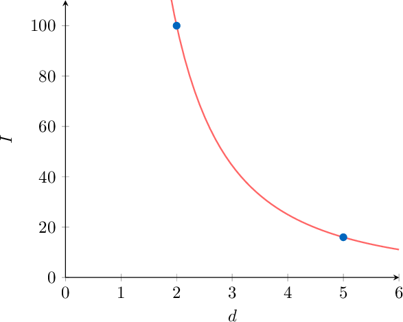
The intensity, $I$, of light from a bulb varies inversely with the square of the distance, $d$ metres, from the bulb. At a distance of 2 metres, the intensity is 100 units.

Write an equation connecting $I$ and $d$.
Find the intensity at a distance of 5 metres.

Answer

Equation: We have $I \propto \frac{1}{d^2}$, so $I = \frac{k}{d^2}$. Using $I=100$ when $d=2$: $$ 100 = \frac{k}{2^2} \implies 100 = \frac{k}{4} \implies k = 400. $$ Hence $I = \frac{400}{d^2}$.
Prediction: When $d=5$: $$ I = \frac{400}{5^2} = \frac{400}{25} = 16 \text{ units}. $$

Skills to practice

Applying Direct and Inverse Variation

VII Solving Systems with Technology

Recappreviously studied — click to reread

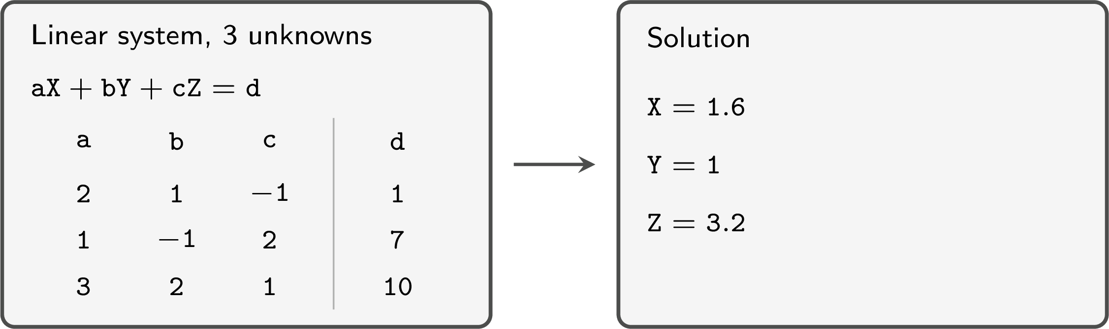
Method — Solving a Linear System with the Equation Solver

The linear system solver, in the equation menu of a graphing calculator, solves a system of two linear equations in two unknowns, or of three linear equations in three unknowns.

Write each equation in the form $ax + by = c$ (two unknowns) or $ax + by + cz = d$ (three unknowns): the unknowns on the left, in the same order in every equation, and the constant on the right.
Open the linear system solver and choose the number of unknowns.
Enter the coefficients row by row, one row per equation, each with its sign, and $0$ for a missing unknown.
Solve and read the value of each unknown. If the solver reports no solution, or infinitely many, the system has no unique solution.
Check the solution by substituting it in each original equation, then report each value exactly when the checks hold exactly, otherwise to 3 significant figures.

The mock-up solves $\begin{cases} 2x + y - z = 1 \\ x - y + 2z = 7 \\ 3x + 2y + z = 10 \end{cases}$: the solution is $x = 1.6$, $y = 1$ and $z = 3.2$. Check: $2 \times 1.6 + 1 - 3.2 = 1$, $1.6 - 1 + 2 \times 3.2 = 7$ and $3 \times 1.6 + 2 \times 1 + 3.2 = 10$, exactly, so these values are exact.

Skills to practice

Solving Systems with Technology

VIII Finding the Parameters of a Model

Method — Finding the Parameters of a Model from Data Points

When the form of a model is known but its parameters are not, data points give the parameters.

Choose the form of the model from the context or from the shape of the data, and count its unknown parameters.
Substitute each data point $(x, y)$ in the model: each point gives one equation whose unknowns are the parameters. When each parameter only multiplies a known expression in $x$ — a polynomial model, or a model such as $\frac{a}{x} + b$ — these equations are linear in the parameters, even when the model is not linear in $x$. A value read directly, such as the value at $x = 0$ of a polynomial model, gives a parameter at once and removes one unknown.
Solve the system with the linear system solver. Use as many data points as unknown parameters, so that the system has as many equations as unknowns, and check that the solver shows a unique solution. If it reports infinitely many, the points do not fix the parameters: replace one of them. If it reports no solution, no model of this form passes through all the points: reconsider the data or the form of the model.
Check the parameters with every data point, then write the model.
State the domain on which the model is used and, when another data point is available, test the model on it.

Example

A ball is thrown upwards. Its height $h$, in metres, $t$ seconds after the throw, is recorded three times: $6.75$ m at $t = 0.5$, $9$ m at $t = 1$ and $6$ m at $t = 2$. The height is modelled by $h(t) = at^2 + bt + c$.

Use technology to find $a$, $b$ and $c$.
Interpret the parameter $c$.
Use technology to find when the ball hits the ground, and state the domain of the model.

Answer

Each reading gives one equation in $a$, $b$ and $c$:
- $(0.5, 6.75)$: $a \times 0.5^2 + b \times 0.5 + c = 6.75$, that is $0.25a + 0.5b + c = 6.75$;
- $(1, 9)$: $a \times 1^2 + b \times 1 + c = 9$, that is $a + b + c = 9$;
- $(2, 6)$: $a \times 2^2 + b \times 2 + c = 6$, that is $4a + 2b + c = 6$.
The linear system solver, with three unknowns and the rows $0.25$, $0.5$, $1$, $6.75$, then $1$, $1$, $1$, $9$, then $4$, $2$, $1$, $6$, displays $a = -5$, $b = 12$ and $c = 2$. Check: $-5 \times 0.25 + 12 \times 0.5 + 2 = 6.75$, $-5 + 12 + 2 = 9$ and $-5 \times 4 + 12 \times 2 + 2 = 6$. The model is $h(t) = -5t^2 + 12t + 2$.
$c = h(0) = 2$: the ball leaves the hand $2$ m above the ground.
The ball hits the ground when $h(t) = 0$, that is $-5t^2 + 12t + 2 = 0$. The polynomial solver displays $t = 2.5564660$ and $t = -0.1564660$. The model describes the ball after the throw, so $t \ge 0$: the ball hits the ground after about $2.56$ seconds. The model is used from the throw to the landing, on the domain $0 \le t \le t_1$, where $t_1 \approx 2.56$ is the positive solution.

Example

A workshop makes wooden chairs. The cost per chair, $C$ dollars, when $n$ chairs are made in a week, is modelled by $C = \dfrac{a}{n} + b$. When $100$ chairs are made, the cost is $\dollar 70$ per chair; when $400$ chairs are made, it is $\dollar 40$ per chair.

Use technology to find $a$ and $b$, then interpret them.
Predict the cost per chair when $1\,000$ chairs are made in a week.

Answer

The model is not linear in $n$, but it is linear in $a$ and $b$. Each data point gives one equation:
- $(100, 70)$: $\dfrac{a}{100} + b = 70$, that is $0.01a + b = 70$;
- $(400, 40)$: $\dfrac{a}{400} + b = 40$, that is $0.0025a + b = 40$.
The linear system solver, with two unknowns and the rows $0.01$, $1$, $70$ and $0.0025$, $1$, $40$, displays $a = 4\,000$ and $b = 30$. Check: $\frac{4\,000}{100} + 30 = 70$ and $\frac{4\,000}{400} + 30 = 40$. The model is $C = \dfrac{4\,000}{n} + 30$.
Interpretation: $\frac{a}{n}$ shares $a$ between the $n$ chairs, so $a = 4\,000$ is the fixed weekly cost, in dollars, whatever the number of chairs (rent, machines); $b = 30$ is the cost, in dollars, of the wood and the work for each chair. The cost per chair decreases as $n$ increases and stays above $\dollar 30$. Here $n$ is a whole number of chairs, and the data cover weekly productions from $100$ to $400$ chairs: a prediction outside this range is an extrapolation.
$$C = \frac{4\,000}{1\,000} + 30 = 34.$$ The model predicts a cost of $\dollar 34$ per chair. This is an extrapolation beyond the two data points: it assumes that the fixed cost does not change when production grows.

Example

Each table comes from an experiment. Determine the variation model that each table follows.

The air resistance $R$, in newtons, on a cyclist riding at $v$ metres per second.

$v$ $2$ $4$ $6$ $8$

$R$ $1.2$ $4.8$ $10.8$ $19.2$

Then predict the air resistance at $10$ metres per second.
The time $T$, in hours, that $w$ workers need to paint a hall.

$w$ $2$ $3$ $4$ $6$

$T$ $18$ $12$ $9$ $6$

Answer

$R$ increases with $v$, so we test direct variation with a power of $v$: we compute $\frac{R}{v}$, then $\frac{R}{v^2}$, for every data point.

$v$ $2$ $4$ $6$ $8$

$\frac{R}{v}$ $0.6$ $1.2$ $1.8$ $2.4$

$\frac{R}{v^2}$ $0.3$ $0.3$ $0.3$ $0.3$

The ratio $\frac{R}{v}$ is not constant, so $R$ does not vary directly with $v$. The ratio $\frac{R}{v^2}$ is constant, equal to $0.3$: $R$ varies directly with the square of $v$, $R \propto v^2$, and $R = 0.3v^2$. Check with doubling: from $v = 2$ to $v = 4$, $R$ is multiplied by $\frac{4.8}{1.2} = 4 = 2^2$, as a square law predicts. At $v = 10$: $$R = 0.3 \times 10^2 = 30.$$ The model predicts an air resistance of $30$ newtons.
$T$ decreases when $w$ increases, so we test inverse variation: we compute the product $wT$ for every data point: $2 \times 18 = 36$, $3 \times 12 = 36$, $4 \times 9 = 36$, $6 \times 6 = 36$. The product is constant, so $T$ varies inversely with $w$: $T \propto \frac{1}{w}$ and $T = \frac{36}{w}$. The constant $36$ is the number of hours one worker alone would need.

Skills to practice

Solving Systems and Fitting Models with the Solver
Determining a Variation Model from Data

IX Going further

Skills to practice

Reasoning about Models
Solving Modelling Problems
Quiz

\(v\)	\(2\)	\(4\)	\(6\)	\(8\)
\(R\)	\(1.2\)	\(4.8\)	\(10.8\)	\(19.2\)

\(w\)	\(2\)	\(3\)	\(4\)	\(6\)
\(T\)	\(18\)	\(12\)	\(9\)	\(6\)

\(v\)	\(2\)	\(4\)	\(6\)	\(8\)
\(\frac{R}{v}\)	\(0.6\)	\(1.2\)	\(1.8\)	\(2.4\)
\(\frac{R}{v^2}\)	\(0.3\)	\(0.3\)	\(0.3\)	\(0.3\)