International Baccalaureate · DP 1: Applications and Interpretation HL
Non-Linear Regression
I
What the Chapter Builds On
I.1
The Least Squares Line and r²
Recappreviously studied — click to reread
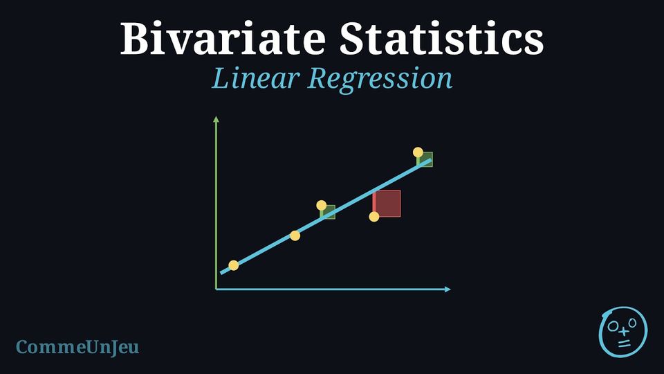
Definition — Least Squares Regression Line
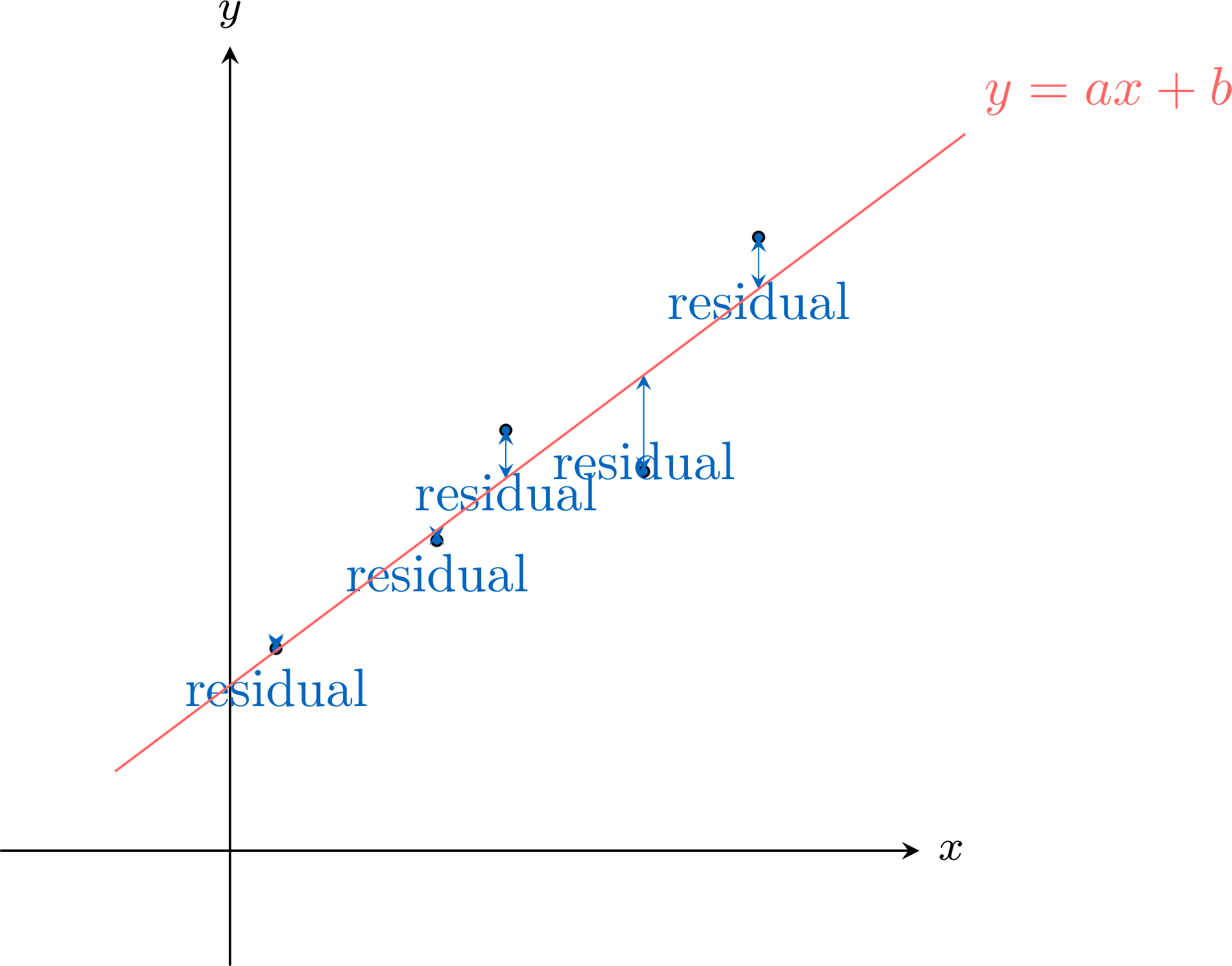
The least squares regression line, written as \(y = ax + b\), is the unique line of best fit (provided the \(x\)-values are not all equal) that models the linear relationship between \(x\) and \(y\). It is calculated by minimising the sum of the squares of the residuals.A residual is the signed vertical difference (positive above the line, negative below) between an observed data point \((x_i, y_i)\) and the predicted point on the regression line \((x_i, \hat{y}_i)\).$$ \text{Residual} = \text{observed } y - \text{predicted } y = y_i - \hat{y}_i $$ A key property is that the least squares regression line always passes through the mean point, \((\bar{x}, \bar{y})\).
Definition — Coefficient of Determination (\(r^2\))
The coefficient of determination (\(r^2\)) is the square of the correlation coefficient. It is a value in the range \([0, 1]\) and is typically expressed as a percentage.The value of \(r^2\) represents the proportion of the variance in the dependent variable (\(y\)) that is explained by the linear relationship with the independent variable (\(x\)). In simple terms, it tells us how well the linear model fits the data.
Method — Obtaining \(r\) and \(r^2\) with Technology
In this method, the correlation coefficient \(r\) is not computed by hand: a calculator or a spreadsheet gives it from the data, together with \(r^2\). - Enter the data: the values of \(x\) in one list (or one column), the values of \(y\) in another, in the same order, so that each pair stays on the same row.
- Ask for the two-variable statistics: on a calculator, the two-variable statistics menu gives \(r\) and \(r^2\); on many models they appear on the linear regression screen \(y = ax + b\), beside the coefficients \(a\) and \(b\) of the least squares line (on some models, the display of \(r\) and \(r^2\) must first be switched on in the settings, and some models show only \(r\)); in a spreadsheet, with \(x\) in
A2:A9and \(y\) inB2:B9, the formula=CORREL(A2:A9,B2:B9)gives \(r\) and=RSQ(B2:B9,A2:A9)gives \(r^2\). - Round only at the end: keep the full value on the screen and give \(r\) and \(r^2\) rounded, usually to three decimal places; \(r^2\) is the square of the unrounded \(r\), so when only \(r\) is displayed, square the full value of \(r\).
- Check with the scatter plot: the sign of \(r\) should agree with the general direction of the cloud, and \(|r|\) with how closely the points follow a line. When they disagree, check that each pair was entered on the same row, and look for an outlier, which can change \(r\) a lot.
Skills to practice
- The Least Squares Line and r²
I.2
Model Families
Recappreviously studied — click to reread
Definition — Cubic Model
A cubic model is a function of the form$$ f(x)=ax^3+bx^2+cx+d, \qquad a\neq 0. $$ - \(a\) determines the overall end behaviour of the graph and its vertical stretch.
- \(d\) is the \(y\)-intercept, since \(f(0)=d\).
Definition — Sine and Cosine Models
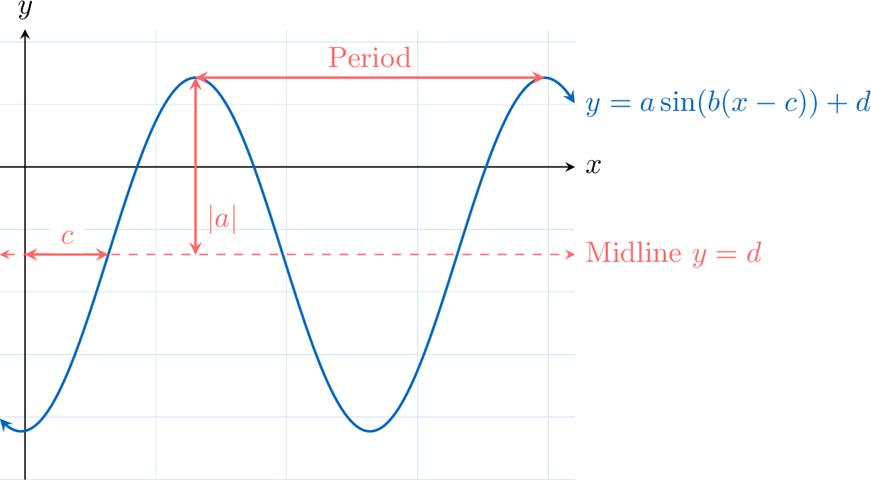
An Sine/Cosine Model is a function of the form $$y = a\sin(b(x-c)) + d\text{ or }y = a\cos(b(x-c)) + d$$ - \(|a|\) is the amplitude.
- \(\frac{2\pi}{|b|}\) (or \(\frac{360}{|b|}\)) is the period.
- \(c\) is the phase shift (horizontal translation).
- \(d\) is the vertical shift (the midline is \(y=d\)).
Definition — Logarithmic Model
A logarithmic model is a function of the form$$ f(x) = a + b\ln x, \qquad x>0,\; b\neq 0. $$ - \(\ln x\) denotes the natural logarithm (base \(e\)).
- \(a\) is the value of the function at \(x=1\), since \(f(1)=a\).
- \(b\) controls the rate of increase/decrease.
Skills to practice
- Model Families
I.3
Semi-Logarithmic and Logarithmic Frames
Recappreviously studied — click to reread
Proposition — Exponential Functions in a Semi-Logarithmic Frame
Let \(k \gt 0\) and \(a \gt 0\). In a semi-logarithmic frame, the points of the curve of \(x \mapsto k \times a^x\) are aligned: their height \(Y = \log y\) satisfies $$\textcolor{colorprop}{Y = \log k + x \log a},$$ a straight line that rises by \(\log a\) decade when \(x\) increases by \(1\) (it falls when \(0 \lt a \lt 1\)), and that meets the vertical axis at the mark \(k\). Conversely, points aligned in a semi-logarithmic frame follow a model \(y = k \times a^x\).
Logarithmic Frames and Power Functions
In a logarithmic frame, both coordinates are replaced by their logarithms. For \(x \gt 0\), the curve of \(x \mapsto k \times x^a\) (\(k \gt 0\)) becomes a straight line of slope \(a\) counted in decades (\(a\) decades up for one decade to the right), whatever the length of a decade on each axis, since \(\log y = \log k + a \log x\). Below, \(y = 3x^2\) for \(1 \le x \le 100\): when \(x\) is multiplied by \(10\) (one decade to the right), \(y\) is multiplied by \(100\) (two decades up). 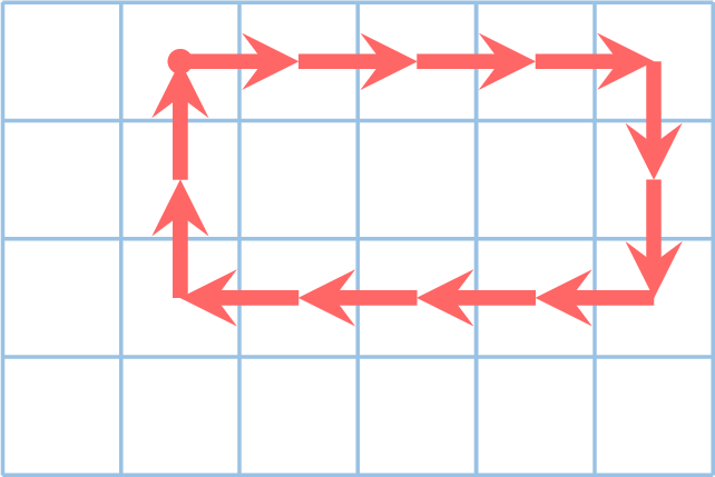
Such frames are used when both quantities span several orders of magnitude: the frequency response of a loudspeaker or of an amplifier (frequencies from \(20\) Hz to \(20\,000\) Hz), the size and the energy needs of animals, the brightness of stars and their distance.
Skills to practice
- Semi-Logarithmic and Logarithmic Frames
II
Linearising Data
II.1
Exponential Models from Data
When the Cloud Bends
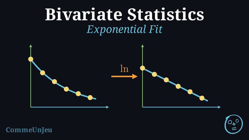
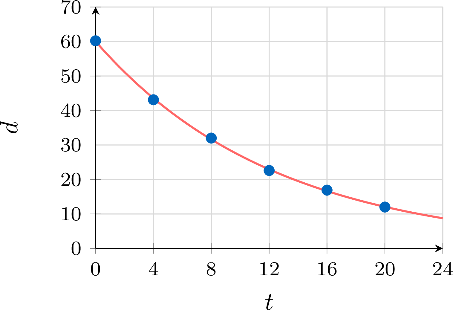
A cup of tea cools down in a room: the difference \(d\) between its temperature and the temperature of the room falls quickly at first, then more and more slowly. The scatter plot of \((t, d)\) is curved, and no line fits it well. When each value of \(d\) is replaced by \(\ln d\), however, the points become almost aligned. A variation in which each step multiplies the quantity by the same factor becomes, through the logarithm, a variation in which each step adds the same amount, since \(\ln\left(k\,q^{t}\right) = \ln k + t\ln q\). This is the idea of a change of variable: transform the data so that an affine fit becomes relevant, fit, then come back to the original variables.
Method — Performing an Exponential Fit
When the scatter plot of \((x_i, y_i)\) looks like the curve of an exponential function and all the \(y_i\) are positive: - Transform: compute \(z_i = \ln y_i\) for each \(i\).
- Check: the points \((x_i, z_i)\) are almost aligned, and the coefficient \(r\) of the series \((x, z)\) is close to \(1\) or to \(-1\).
- Fit: determine the least squares line \(z = ax + b\) of \(z\) on \(x\).
- Come back: \(\ln y = ax + b\) is equivalent to \(y = e^{ax + b} = e^{b} \times \left(e^{a}\right)^{x}\), that is \(y = k\,q^{x}\) with \(k = e^{b} > 0\) and \(q = e^{a} > 0\).
Example
A cup of tea is left in a room. Every \(4\) minutes, the difference \(d\), in degrees Celsius, between its temperature and the temperature of the room is recorded. | Time \(t\) (min) | \(0\) | \(4\) | \(8\) | \(12\) | \(16\) | \(20\) |
| Difference \(d\) (\(^\circ\)C) | \(60.2\) | \(43.1\) | \(32.0\) | \(22.6\) | \(16.9\) | \(12.0\) |
- Compute the values \(z_i = \ln d_i\) rounded to \(10^{-3}\), then determine the least squares line of \(z\) on \(t\), with the slope rounded to \(10^{-4}\) and the intercept to \(10^{-3}\).
- Deduce an expression of \(d\) as a function of \(t\).
- Estimate the difference after \(30\) minutes, then the time after which the initial difference has been halved.
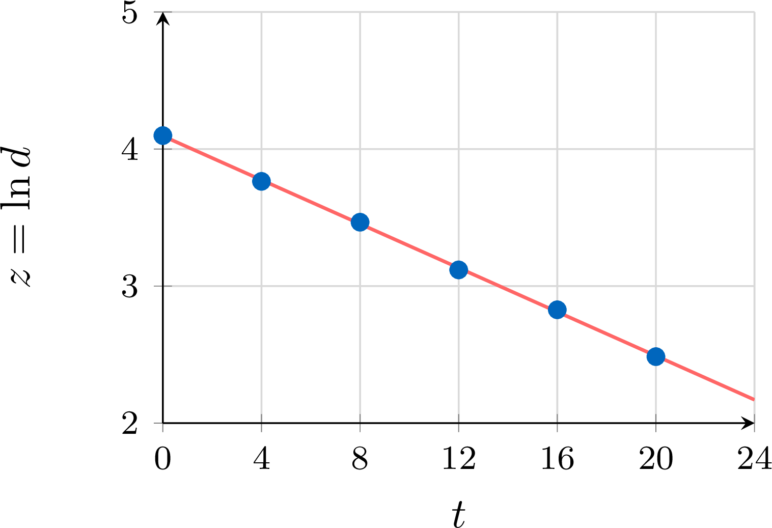
- The values of \(z = \ln d\) are \(4.098\), \(3.764\), \(3.466\), \(3.118\), \(2.827\), \(2.485\). The calculator gives \(z = -0.0802t + 4.095\), with \(r \approx -0.9998\): the points \((t, z)\) are almost aligned.
- \(\ln d = -0.0802t + 4.095\) is equivalent to \(d = e^{4.095} \times \left(e^{-0.0802}\right)^{t}\), that is \(d \approx 60.0 \times 0.923^{t}\).
- After \(30\) minutes, \(d \approx e^{4.095 - 0.0802 \times 30} = e^{1.689} \approx 5.4\) \(^\circ\)C. The value \(t = 30\) lies outside the observations, so this estimate assumes that the cooling goes on in the same way. The difference is halved when \(e^{-0.0802t} = \dfrac{1}{2}\), that is \(-0.0802t = -\ln 2\), so \(t = \dfrac{\ln 2}{0.0802} \approx 8.6\) minutes.
Skills to practice
- Fitting an Exponential Model
- Modelling with an Exponential Fit
II.2
Power and Logarithmic Models from Data
Other Changes of Variable
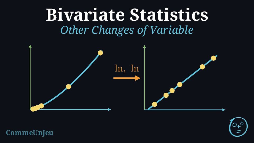
The same approach applies whenever a transformation makes the cloud straight. The transformation must be defined for all the data, and the return to the original variables must be possible on the values considered.
| Change of variable | Condition | Fitted line | Model after return |
| \(u = \ln x\) | \(x > 0\) | \(y = au + b\) | \(y = a\ln x + b\) |
| \(u = \dfrac{1}{x}\) | \(x \neq 0\) | \(y = au + b\) | \(y = \dfrac{a}{x} + b\) |
| \(u = x^2\) | none | \(y = au + b\) | \(y = ax^2 + b\) |
| \(w = \sqrt{y}\) | \(y \geq 0\) | \(w = ax + b\) | \(y = (ax + b)^2\) where \(ax + b \geq 0\) |
| \(w = y^2\) | \(y \geq 0\) | \(w = ax + b\) | \(y = \sqrt{ax + b}\) where \(ax + b \geq 0\) |
| \(u = \ln x\), \(v = \ln y\) | \(x > 0\), \(y > 0\) | \(v = au + b\) | \(y = e^{b}\,x^{a}\) |
Example
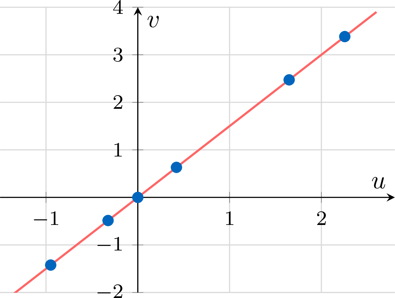
Kepler's third law. For six planets, the table gives the mean distance \(D\) to the Sun (the semi-major axis of its orbit), in astronomical units, and the period of revolution \(T\), in years, with the values of \(u = \ln D\) and \(v = \ln T\) rounded to \(10^{-3}\). | Planet | Mercury | Venus | Earth | Mars | Jupiter | Saturn |
| \(D\) | \(0.387\) | \(0.723\) | \(1.000\) | \(1.524\) | \(5.203\) | \(9.537\) |
| \(T\) | \(0.241\) | \(0.615\) | \(1.000\) | \(1.881\) | \(11.862\) | \(29.457\) |
| \(u = \ln D\) | \(-0.949\) | \(-0.324\) | \(0.000\) | \(0.421\) | \(1.649\) | \(2.255\) |
| \(v = \ln T\) | \(-1.423\) | \(-0.486\) | \(0.000\) | \(0.632\) | \(2.473\) | \(3.383\) |
- Determine the least squares line of \(v\) on \(u\), with coefficients rounded to \(10^{-3}\).
- Deduce a relation between \(T\) and \(D\).
- The calculator gives \(v = 1.500u + 0.000\), with \(r \approx 1.000\): the points \((u, v)\) are almost aligned.
- The fit gives \(\ln T \approx 1.5\ln D\); exponentiating, \(T \approx e^{1.5\ln D} = D^{1.5}\), a small gap between the logarithms meaning a small relative gap between the values, that is \(T^2 \approx D^3\) with these units. The fit recovers, from six measured values, the relation stated by Kepler in 1619 and later explained by Newton's theory of gravitation: the square of the period is proportional to the cube of the distance.
Judging a Fit after a Change of Variable
The least squares criterion applies to the transformed values: after an exponential fit, it is the gaps between the \(z_i = \ln y_i\) and the line that are made minimal, not the gaps between the \(y_i\) and the curve. An affine fit of \((x, y)\) and a fit of \((x, \ln y)\) therefore do not minimise errors measured on the same scale, and their coefficients \(r\) are not scores that can be compared. To choose between two models, compare the gaps \(y_i - \hat{y}_i\) between the observed values and the values \(\hat{y}_i\) predicted by each model, in the original units; look at the shape of the cloud; and use the context: a model that predicts a negative price, or a quantity that grows without limit where a limit is known, is rejected whatever its coefficient.
Skills to practice
- Choosing a Change of Variable
II.3
Changes of Variable with the Common Logarithm and with Powers
Straightening a Curved Cloud
When a scatter plot is clearly curved, a line fits it poorly, and a least squares line computed anyway can give absurd predictions. A change of variable replaces one of the two variables by a function of it, chosen so that the new points are almost aligned: an affine fit then becomes relevant for the new variables, and a model for the original variables is deduced from it. Two families of changes cover most situations met in practice.
- A power or an inverse of \(x\) — \(x^2\), \(\dfrac{1}{x}\), \(\dfrac{1}{\sqrt{x}}\) — straightens a cloud in which \(y\) grows like the square of \(x\) (a distance travelled from rest, an area), or falls like its inverse (a pressure, a cost shared among more and more items).
- The common logarithm of \(y\) straightens a cloud in which each step of \(x\) multiplies \(y\) by the same factor, because it turns products into sums: \(\log\left(k \times q^{x}\right) = \log k + x \log q\), an affine expression of \(x\).
Method — Fitting after a Change of Variable
The usual changes of variable, and the model obtained after coming back to the original variables: | Change of variable | Condition on the data | Line at the calculator | Model after coming back |
| \(u = x^2\) | none | \(y = au + b\) | \(y = ax^2 + b\) |
| \(u = \dfrac{1}{x}\) | \(x \neq 0\) | \(y = au + b\) | \(y = \dfrac{a}{x} + b\) |
| \(u = \dfrac{1}{\sqrt{x}}\) | \(x \gt 0\) | \(y = au + b\) | \(y = \dfrac{a}{\sqrt{x}} + b\) |
| \(z = \log y\) | \(y \gt 0\) | \(z = ax + b\) | \(y = k \times q^{x}\), \(k = 10^{b}\), \(q = 10^{a}\) |
- Choose the change of variable from the shape of the cloud and from the context, and check that it is defined for all the data.
- Transform: compute the new values (\(u_i\) or \(z_i\)), rounded as the statement asks, and check that the new points are almost aligned.
- Fit: enter the transformed series at the calculator and ask for the least squares line, as for any two-variable series.
- Come back to the original variables. For \(z = \log y\): \(\log y = ax + b\) means \(y = 10^{ax + b}\), that is \(y = 10^{b} \times \left(10^{a}\right)^{x}\); each increase of \(x\) by \(1\) multiplies \(y\) by \(q = 10^{a}\), and \(\log q = a\).
- Use the model with care: inside the range of the data it interpolates; outside, it extrapolates, and only the context says whether the variation goes on in the same way.
Example
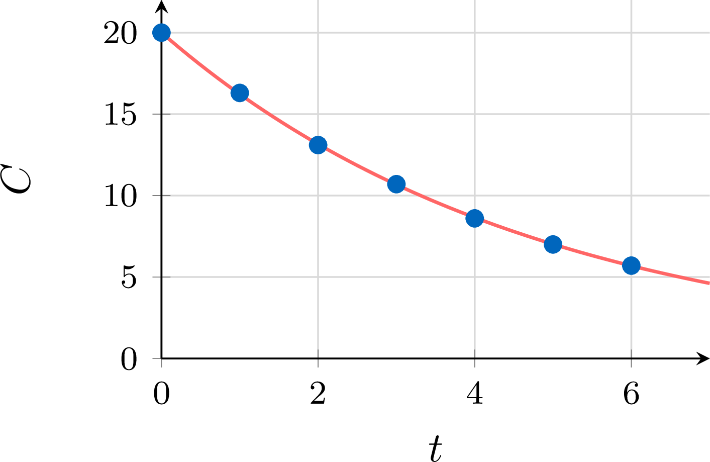
After an injection, the concentration \(C\) of a medicine in the blood, in milligrams per litre, is measured every hour. | Time \(t\) (h) | \(0\) | \(1\) | \(2\) | \(3\) | \(4\) | \(5\) | \(6\) |
| \(C\) (mg/L) | \(20.0\) | \(16.3\) | \(13.1\) | \(10.7\) | \(8.6\) | \(7.0\) | \(5.7\) |
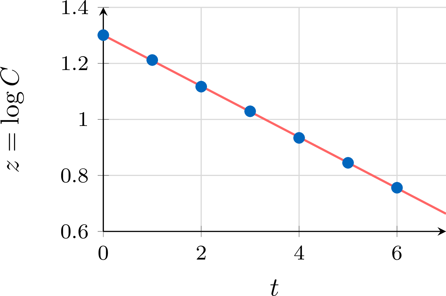
- Compute the values \(z = \log C\) rounded to \(10^{-3}\), then determine at the calculator the least squares line of \(z\) on \(t\), with the slope rounded to \(10^{-4}\) and the intercept to \(10^{-3}\).
- Deduce an expression of \(C\) as a function of \(t\), in the form \(C = k \times q^{t}\) with \(k\) rounded to \(10^{-1}\) and \(q\) to \(10^{-3}\). By what percentage does the concentration fall each hour?
- Estimate the concentration after \(2\) h \(30\) min, then the time after which the initial concentration has been halved.
- The values of \(z = \log C\) are \(1.301\), \(1.212\), \(1.117\), \(1.029\), \(0.934\), \(0.845\), \(0.756\): the points \((t, z)\) are almost aligned. The calculator gives \(z = -0.0911t + 1.301\).
- \(\begin{aligned}[t] \log C &= -0.0911t + 1.301 \\ C &= 10^{-0.0911t + 1.301} &&\text{(definition of the common logarithm)}\\ &= 10^{1.301} \times \left(10^{-0.0911}\right)^{t} &&\text{(properties of the powers)}\\ &\approx 20.0 \times 0.811^{t} \end{aligned}\)
Each hour multiplies the concentration by \(0.811\): it falls by \(1 - 0.811 = 0.189\), that is by about \(18.9\pourcent\) per hour. - After \(2\) h \(30\) min, \(t = 2.5\): \(C \approx 20.0 \times 0.811^{2.5} \approx 11.8\) mg/L; \(2.5\) lies between \(0\) and \(6\), so this is an interpolation. The concentration is halved when \(q^{t} = \dfrac{1}{2}\):
\(\begin{aligned}[t] t \log q &= \log 0.5 &&\text{(logarithm of a power)}\\ t &= \dfrac{\log 0.5}{-0.0911} &&\text{(}\log q = a\text{)}\\ &\approx 3.3 \end{aligned}\)
The concentration is halved after about \(3.3\) hours, that is about \(3\) h \(18\) min.
Example
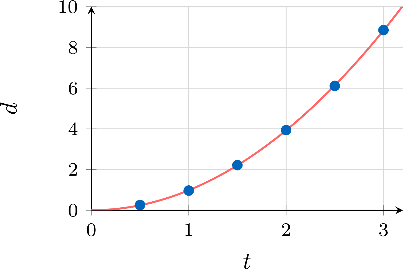
A ball is released without speed at the top of a slightly sloping rail; the distance \(d\) it has travelled, in metres, is measured \(t\) seconds after its release. | Time \(t\) (s) | \(0.5\) | \(1.0\) | \(1.5\) | \(2.0\) | \(2.5\) | \(3.0\) |
| Distance \(d\) (m) | \(0.26\) | \(0.97\) | \(2.22\) | \(3.94\) | \(6.11\) | \(8.85\) |
- The least squares line of \(d\) on \(t\) is \(d = 3.434t - 2.284\). What distance does it predict for \(t = 0.5\)? Comment.
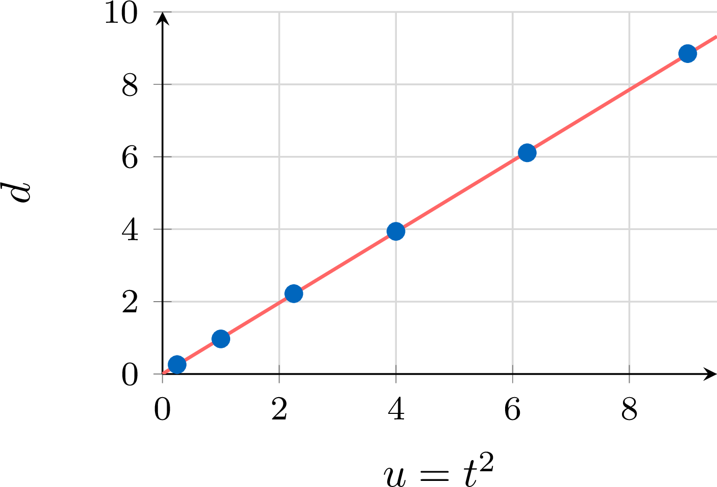
- Compute the values \(u = t^2\), then determine at the calculator the least squares line of \(d\) on \(u\), with coefficients rounded to \(10^{-3}\).
- Deduce an expression of \(d\) as a function of \(t\), then estimate the distance travelled after \(2.2\) seconds.
- \(3.434 \times 0.5 - 2.284 \approx -0.57\) m: a negative distance, which is absurd. The cloud \((t, d)\) is curved — the distance grows faster and faster — and a line does not describe it.
- The values of \(u = t^2\) are \(0.25\), \(1\), \(2.25\), \(4\), \(6.25\), \(9\): the points \((u, d)\) are almost aligned. The calculator gives \(d = 0.981u + 0.004\).
- \(d \approx 0.981t^2 + 0.004\): the intercept is almost \(0\), so the distance is about proportional to the square of the time, \(d \approx 0.98\,t^2\), as the physics of motion from rest predicts. After \(2.2\) s: \(d \approx 0.981 \times 2.2^2 + 0.004 \approx 4.75\) m, an interpolation since \(2.2\) lies between \(0.5\) and \(3\).
Example
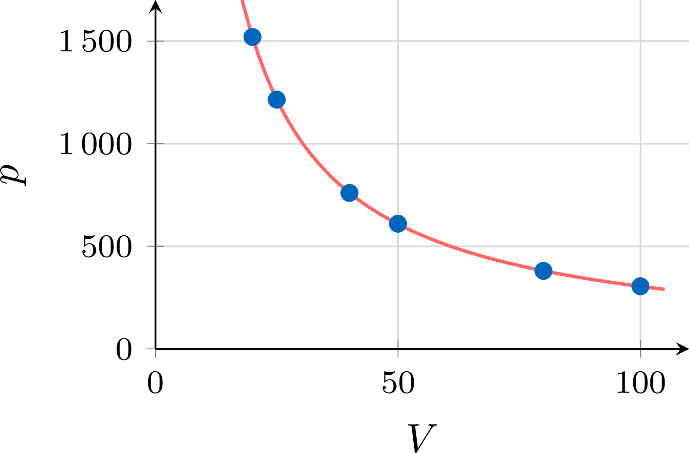
The air enclosed in a syringe is compressed slowly, at constant temperature; its pressure \(p\), in hectopascals, is read for several volumes \(V\), in millilitres. | Volume \(V\) (mL) | \(20\) | \(25\) | \(40\) | \(50\) | \(80\) | \(100\) |
| Pressure \(p\) (hPa) | \(1520\) | \(1215\) | \(760\) | \(610\) | \(380\) | \(305\) |
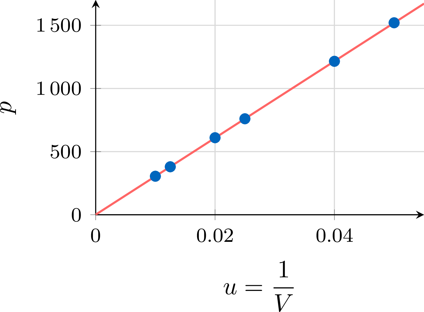
- Compute the values \(u = \dfrac{1}{V}\), then determine at the calculator the least squares line of \(p\) on \(u\), with coefficients rounded to the unit.
- Deduce an expression of \(p\) as a function of \(V\), and interpret the intercept.
- Estimate the pressure for a volume of \(35\) mL.
- The values of \(u = \dfrac{1}{V}\) are \(0.05\), \(0.04\), \(0.025\), \(0.02\), \(0.0125\), \(0.01\): the points \((u, p)\) are almost aligned. The calculator gives \(p = 30\,366u + 1\).
- \(p \approx \dfrac{30\,366}{V} + 1\). The intercept, about \(1\) hPa, is negligible beside pressures of several hundred hectopascals: \(p \approx \dfrac{30\,366}{V}\), that is \(pV \approx 30\,366\). The product of the pressure and the volume stays about constant: this is the Boyle–Mariotte law.
- \(p \approx \dfrac{30\,366}{35} + 1 \approx 867.6 + 1 \approx 869\) hPa, an interpolation since \(35\) lies between \(20\) and \(100\).
Skills to practice
- Fitting after a Change of Variable
- Fitting with Technology in Context
III
Predicting with a Fit
III.1
Interpolation and Extrapolation
Recappreviously studied — click to reread
The Study Domain
A fit \(y = f(x)\) turns the series into a model that can estimate \(y\) for a value of \(x\) that was not observed, or, when the equation \(f(x) = y\) has a single solution, \(x\) for a given value of \(y\). The study domain is the interval from the smallest to the largest observed value of \(x\). Inside it, an estimate is an interpolation: it relies on the observations around it, and it is reasonable when the model fits the data well. Outside it, an estimate is an extrapolation: it relies on an extra hypothesis, that the trend goes on beyond the observations, which the data alone can never guarantee. The further from the study domain, the more fragile the estimate. When \(x\) is time, extrapolating beyond the last observation is forecasting: the forecast must be given with its hypothesis and with words such as “about” or “if the trend continues”.
Example
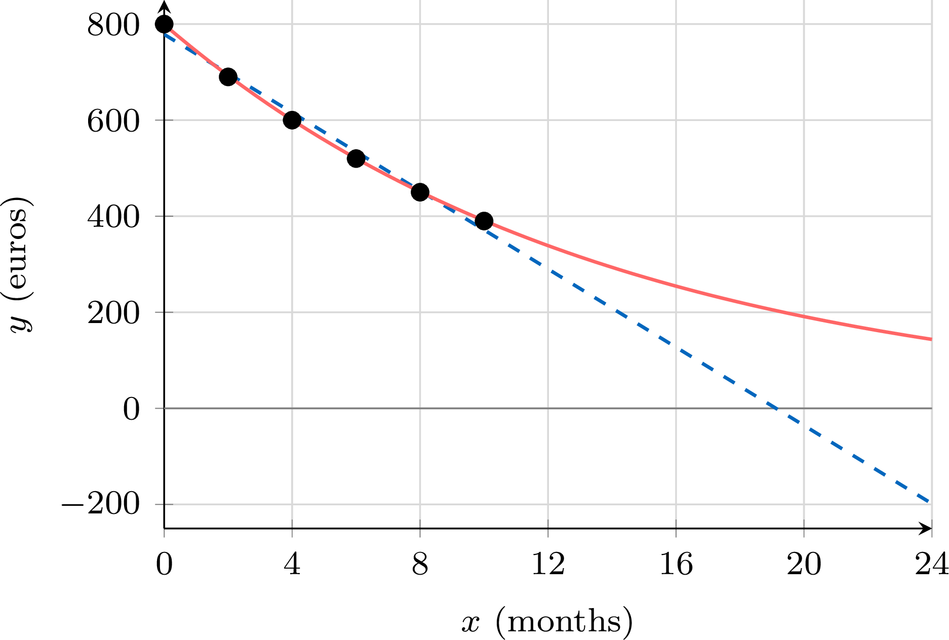
The price \(y\), in euros, of a smartphone model is recorded every two months after its release, \(x\) being the number of months. | Months \(x\) | \(0\) | \(2\) | \(4\) | \(6\) | \(8\) | \(10\) |
| Price \(y\) (euros) | \(800\) | \(690\) | \(600\) | \(520\) | \(450\) | \(390\) |
- The least squares line is \(y = -40.71x + 778.6\), with \(r \approx -0.994\). Estimate the price after \(5\) months, then after \(24\) months, and comment.
- An exponential fit gives \(y \approx 799 \times 0.931^{x}\). Compare the gaps between the observed prices and the prices predicted by each model, then estimate the price after \(24\) months with the exponential model.
- After \(5\) months, an interpolation: \(-40.71 \times 5 + 778.6 \approx 575\) euros. After \(24\) months, an extrapolation: \(-40.71 \times 24 + 778.6 \approx -198\) euros, a negative price, which is absurd. The line reaches \(0\) for \(x \approx 19\) months: the affine trend cannot go on, even though \(|r|\) is close to \(1\).
- Gaps \(y_i - \hat{y}_i\) for the six observations, computed with the two models above and rounded to one decimal place:
\(x\) \(0\) \(2\) \(4\) \(6\) \(8\) \(10\) Affine model \(21.4\) \(-7.2\) \(-15.8\) \(-14.3\) \(-2.9\) \(18.5\) Exponential model \(1.0\) \(-2.5\) \(-0.3\) \(-0.3\) \(-1.0\) \(-0.9\)
Skills to practice
- Recognising Interpolation and Extrapolation
IV
Non-Linear Regression
IV.1
Least Squares Regression Curves
When No Change of Variable Straightens the Cloud
A ball thrown upwards rises, then falls; the mean temperature of a city rises and falls with the seasons. The points of such scatter diagrams follow a curve that changes direction, and the usual changes of variable (\(\ln x\), \(\ln y\), \(x^2\), \(\frac{1}{x}\)) do not make them aligned: a logarithm straightens a quantity that is multiplied by the same factor at each step, not a quantity that goes up and then down, and a new variable such as \((x - c)^2\) would first require the position \(c\) of the turning point, which is unknown. A model with three parameters, such as \(y = ax^2 + bx + c\), cannot be read off one line either, since a line gives only two coefficients. The idea of least squares still applies: within a family of curves chosen for the situation — the parabolas, the cubic curves, the sine curves —, keep the curve whose vertical gaps with the points, squared and added, are the smallest. Technology carries out the search; choosing the family, reading the result and judging the fit remain the work of whoever builds the model.
Definition — Residuals and the Sum of Square Residuals
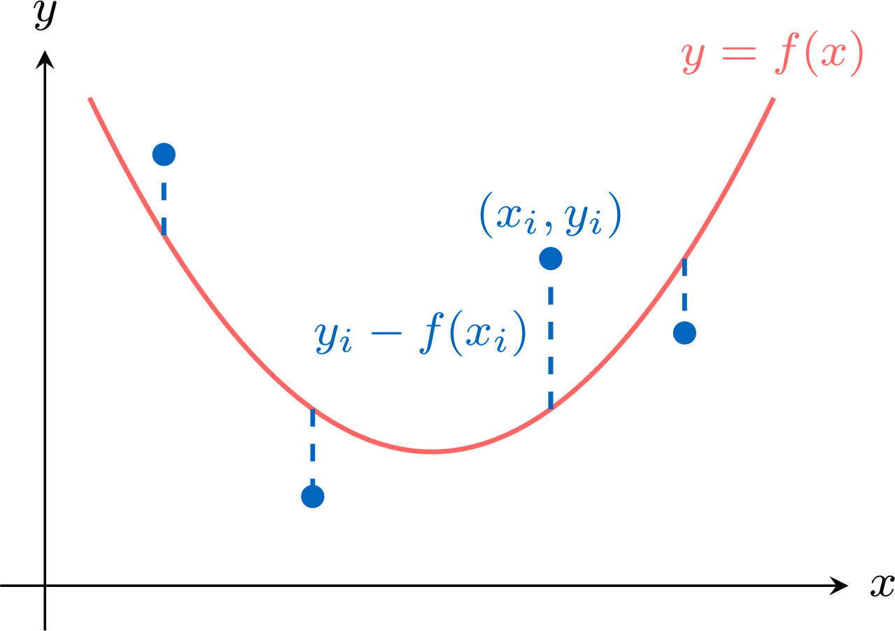
Let \((x_1, y_1), (x_2, y_2), \ldots, (x_n, y_n)\) be bivariate data and \(y = f(x)\) a model of \(y\) in terms of \(x\). - The residual of the point \((x_i, y_i)\) is \(y_i - f(x_i)\), the observed value minus the value predicted by the model: positive when the point lies above the curve, negative when it lies below, as for a line.
- The sum of square residuals of the model is $$SS_{\text{res}} = \sum_{i=1}^{n} \left(y_i - f(x_i)\right)^2.$$ It is expressed in the square of the unit of \(y\), and it is \(0\) exactly when the curve passes through every point.
- Among the models of a family (for instance all the parabolas \(y = ax^2 + bx + c\)), the least squares regression curve is the model whose sum of square residuals is the smallest.
Definition — Coefficient of Determination of a Model
Let \(\bar{y}\) be the mean of \(y_1, y_2, \ldots, y_n\), these values not being all equal. The total sum of squares $$SS_{\text{tot}} = \sum_{i=1}^{n} \left(y_i - \bar{y}\right)^2$$ measures the variability of \(y\) around its mean; it is the sum of square residuals of the constant model \(y = \bar{y}\). The coefficient of determination of a model \(y = f(x)\) is $$R^2 = 1 - \frac{SS_{\text{res}}}{SS_{\text{tot}}}.$$ For the least squares curve of a family that contains the constant models, it lies between \(0\) and \(1\) (Proposition “Properties of the Coefficient of Determination”) and gives the proportion of the variability of \(y\) accounted for by the model: \(R^2 = 0.95\) means that the model accounts for \(95\pourcent\) of the variability of \(y\). A model that is further from the points than the constant model \(y = \bar{y}\) has a negative \(R^2\). The coefficient of determination is read on the scale of \(y\), since it is computed from the residuals of \(y\). Proposition — Properties of the Coefficient of Determination
Let the values \(y_1, y_2, \ldots, y_n\) be not all equal. The quadratic and the cubic regressions choose among the polynomial curves of degree at most \(2\) and of degree at most \(3\), which include the constant models. - For the least squares regression curve of a family that contains the constant models — the least squares line, the quadratic and the cubic regression curves —, \(0 \le R^2 \le 1\), and \(R^2 = 1\) exactly when the curve passes through every point.
- For the least squares line, the values \(x_1, x_2, \ldots, x_n\) being not all equal either, \(R^2 = r^2\), the square of Pearson's correlation coefficient.
- When every model of a family belongs to a larger family (a polynomial of degree at most \(2\) is a polynomial of degree at most \(3\) whose coefficient of \(x^3\) is \(0\)), the least squares curve of the larger family has an \(SS_{\text{res}}\) at most equal and an \(R^2\) at least equal: adding a term to a model never lowers \(R^2\).
- The constant model \(y = \bar{y}\) belongs to the family (a constant is a polynomial of degree at most \(2\), or at most \(3\)), and its sum of square residuals is \(SS_{\text{tot}}\). The least squares curve has the smallest sum of square residuals of the family, and a sum of squares is never negative, so \(0 \le SS_{\text{res}} \le SS_{\text{tot}}\). Since \(SS_{\text{tot}} > 0\): $$\begin{aligned}[t] R^2 &= 1 - \frac{SS_{\text{res}}}{SS_{\text{tot}}} \\ &\ge 1 - \frac{SS_{\text{tot}}}{SS_{\text{tot}}} && \text{(}SS_{\text{res}} \le SS_{\text{tot}}\text{)}\\ &= 0, \end{aligned}$$ and \(R^2 \le 1\) because \(\frac{SS_{\text{res}}}{SS_{\text{tot}}} \ge 0\). Finally, \(R^2 = 1\) exactly when \(SS_{\text{res}} = 0\), that is when every residual is \(0\), since a sum of squares is \(0\) only when each of its terms is \(0\).
- This equality follows from the formulas of the coefficients of the least squares line; it is admitted here.
- The least squares curve of the smaller family is one of the curves of the larger family. The least squares curve of the larger family has the smallest sum of square residuals among all its curves, so its \(SS_{\text{res}}\) is at most that of the first curve. Both coefficients of determination use the same \(SS_{\text{tot}}\), which depends only on the data: the smaller \(SS_{\text{res}}\) gives the larger \(R^2\).
Method — Fitting a Regression Curve with Technology
- Enter and look: the values of \(x\) in one list, those of \(y\) in another, in the same order; draw the scatter diagram and choose a family from the shape of the cloud and from the context.
- Ask for the regression in the two-variable statistics menu: quadratic \(y = ax^2 + bx + c\) (
QuadRegon many models), cubic \(y = ax^3 + bx^2 + cx + d\) (CubicReg), exponential \(y = a \times b^x\) (ExpReg, all the \(y\)-values positive; some models also offer \(y = a\,e^{bx}\)), power \(y = a \times x^b\) (PwrReg, all the \(x\)- and \(y\)-values positive), sine \(y = a\sin(bx + c) + d\) (SinReg, which works in radians and needs \(x\)-values in increasing order and equally spaced, or an estimate of the period). The letters \(a\), \(b\), \(c\), \(d\) are those of the calculator: write the model with the letters of the situation. - Store the equation and draw it over the scatter diagram: the curve should follow the cloud.
- Read the coefficient of determination where it is displayed (on some models, the display of the statistics diagnostics must first be switched on).
- Compute \(SS_{\text{res}}\) when it is needed: in a third list, or column, the squares \(\left(y - f(x)\right)^2\) computed with the stored equation, then their sum.
- Round only at the end: predictions and residuals are computed with the stored equation, not with rounded coefficients.
| Regression | Least squares on | Coefficient displayed |
| quadratic, cubic | \(y\) | \(R^2\), scale of \(y\) |
| logarithmic \(y = a + b\ln x\) | \(y\) (line of \(y\) on \(\ln x\)) | \(r^2\), scale of \(y\) |
| exponential | \(\ln y\) (line of \(\ln y\) on \(x\)) | \(r^2\), scale of \(\ln y\) |
| power | \(\ln y\) (line of \(\ln y\) on \(\ln x\)) | \(r^2\), scale of \(\ln y\) |
| sine | \(y\), by successive approximations | none |
Example
A ball is thrown upwards. A video gives its height \(h\) above the ground, in metres, \(t\) seconds after the throw. | \(t\) (s) | \(0\) | \(0.4\) | \(0.8\) | \(1.2\) | \(1.6\) | \(2.0\) | \(2.4\) |
| \(h\) (m) | \(1.6\) | \(5.4\) | \(8.1\) | \(8.7\) | \(8.3\) | \(5.8\) | \(2.1\) |
- Use technology to fit a quadratic model \(h = at^2 + bt + c\), with the coefficients to \(3\) significant figures, and give \(R^2\) to \(3\) decimal places.
- Calculate the residuals, to \(2\) decimal places, and the sum of square residuals, to \(3\) decimal places.
- Use the model to estimate the greatest height of the ball, and the time at which it reaches the ground.
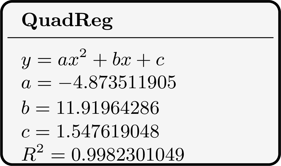
- With \(t\) in L1 and \(h\) in L2, the quadratic regression gives the screen below.
- Each residual is \(h - \hat{h}\), where \(\hat{h}\) is the height given by the stored equation:
\(t\) \(0\) \(0.4\) \(0.8\) \(1.2\) \(1.6\) \(2.0\) \(2.4\) \(\hat{h}\) \(1.55\) \(5.54\) \(7.96\) \(8.83\) \(8.14\) \(5.89\) \(2.08\) \(h - \hat{h}\) \(0.05\) \(-0.14\) \(0.14\) \(-0.13\) \(0.16\) \(-0.09\) \(0.02\) 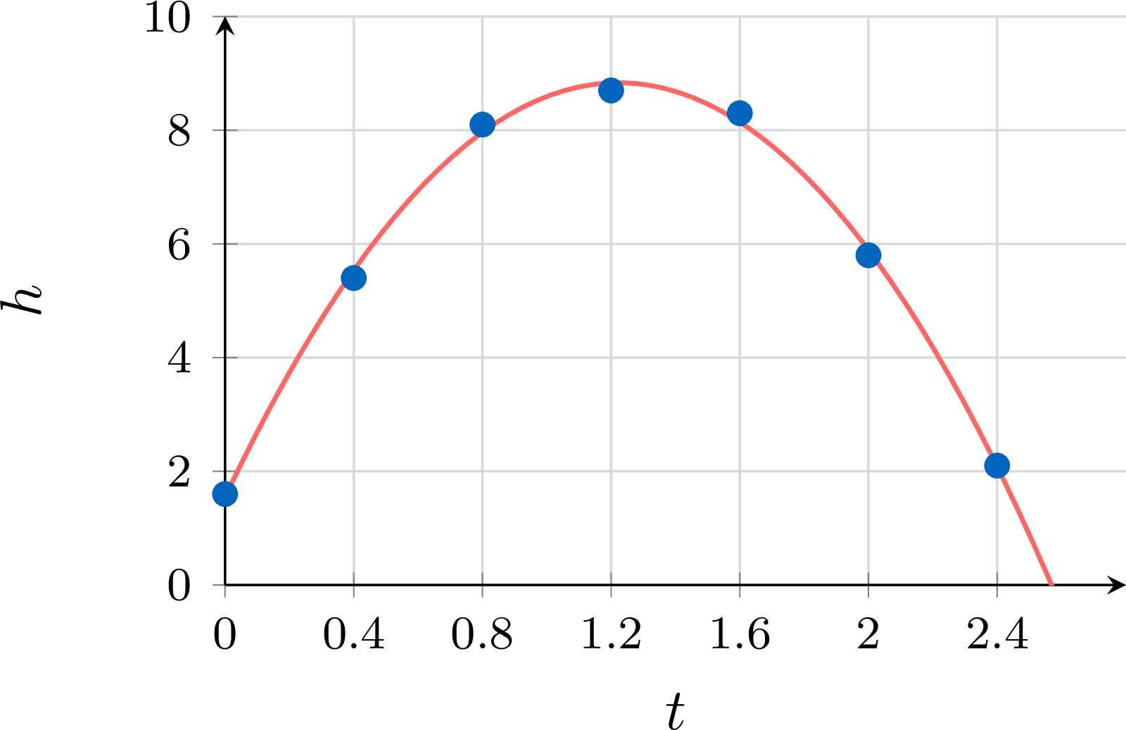
- The greatest height is reached at the vertex of the parabola, for $$\begin{aligned}[t] t &= -\frac{b}{2a} && \text{(vertex of a parabola)}\\ &= -\frac{11.919\ldots}{2 \times (-4.8735\ldots)}\\ &\approx 1.22 \text{ s}, \end{aligned}$$ and the stored equation gives \(h \approx 8.84\) m at that time. The ball reaches the ground when \(h = 0\): the equation \(-4.8735\ldots t^2 + 11.919\ldots t + 1.5476\ldots = 0\) has the positive solution \(t \approx 2.57\) s (the other solution, about \(-0.12\), is before the throw). This time lies just beyond the last observation, \(2.4\) s: it is an extrapolation, reasonable here because the ball keeps falling freely until it lands.
Method — Comparing Regression Models
To choose between several models of the same data: - Compare them on one scale: compute the sum of square residuals of each model in the units of \(y\), with its stored equation; for these data, the smaller \(SS_{\text{res}}\), the closer the curve to the points. An \(r^2\) read on the scale of \(\ln y\) is never compared with an \(R^2\) read on the scale of \(y\).
- Count the parameters: a model with more parameters can follow the points more closely. A cubic regression never does worse than a quadratic one, and a polynomial curve of degree \(n - 1\) passes through \(n\) points with distinct \(x\)-values, with \(SS_{\text{res}} = 0\) and \(R^2 = 1\), while its bends between and beyond the points have no meaning. A small gain does not justify an extra parameter.
- Look at the residuals: small residuals whose signs change without a regular pattern suit the family; residuals that keep the same sign over long runs, in a systematic pattern (for instance positive at both ends and negative in the middle), reveal a shape that the model misses.
- Use the context: the behaviour beyond the data (a quantity that cannot become negative, a limit, a period) and the meaning of the parameters. The coefficient of determination alone does not decide.
Example
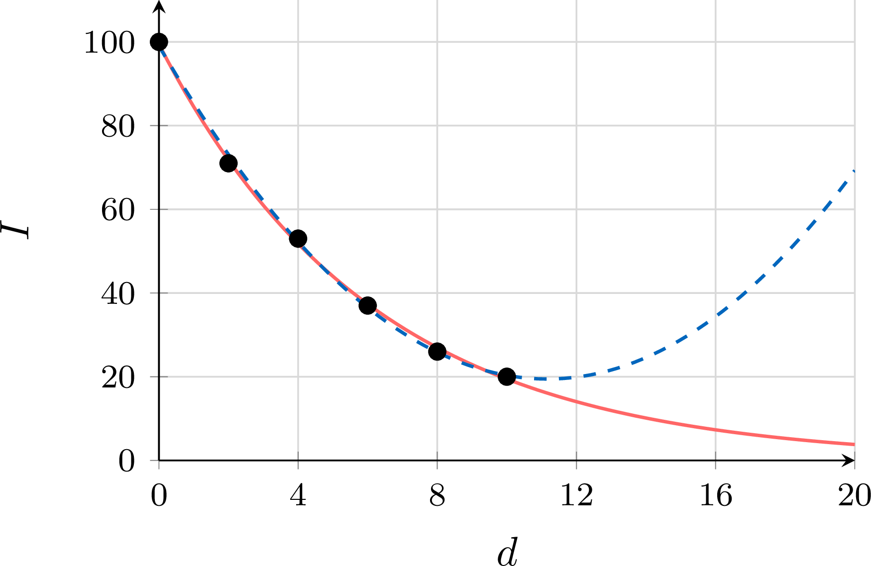
The intensity \(I\) of the light under the surface of a lake, as a percentage of the intensity at the surface, is measured at several depths \(d\), in metres. | \(d\) (m) | \(0\) | \(2\) | \(4\) | \(6\) | \(8\) | \(10\) |
| \(I\) (\%) | \(100\) | \(71\) | \(53\) | \(37\) | \(26\) | \(20\) |
- Use technology to fit an exponential model \(I = a \times b^d\) and a quadratic model \(I = ad^2 + bd + c\), with the coefficients to \(3\) significant figures. Write down the coefficient displayed with each one.
- The quadratic model shows the larger coefficient. Explain why this does not show that it fits the data better.
- Calculate the sum of square residuals of each model on the scale of \(I\), and compare.
- Estimate the intensity at a depth of \(20\) m with each model. Which model should be kept?
- With \(d\) in L1 and \(I\) in L2, the two regressions give the screens below.
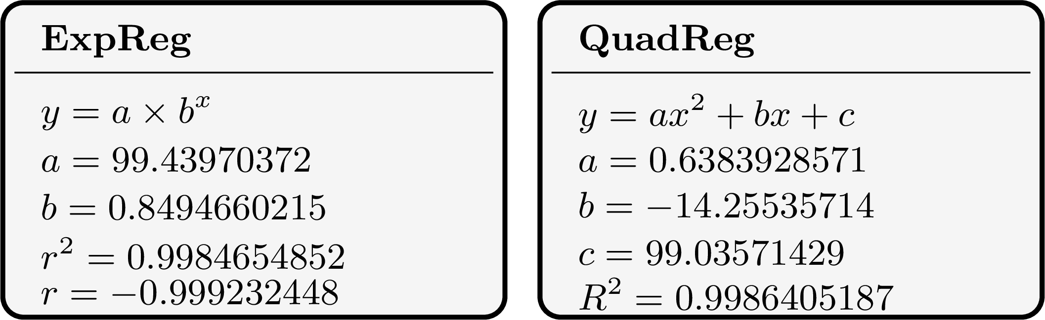
- The exponential regression is the least squares line of \(\ln I\) on \(d\): its \(r^2\) measures how well the points \((d, \ln I)\) are aligned, on the scale of \(\ln I\). The quadratic regression minimises the residuals of \(I\) itself, and its \(R^2\) is read on the scale of \(I\). Two coefficients read on different scales are not compared.
- The residuals are computed with the stored equations, on the scale of \(I\):
\(d\) \(0\) \(2\) \(4\) \(6\) \(8\) \(10\) exponential \(0.56\) \(-0.75\) \(1.22\) \(-0.36\) \(-0.96\) \(0.55\) quadratic \(0.96\) \(-2.08\) \(0.77\) \(0.51\) \(0.15\) \(-0.32\) - At \(20\) m, the exponential model gives \(I \approx 99.4 \times 0.849^{20} \approx 3.8\pourcent\), and the quadratic model \(I \approx 69.3\pourcent\). The parabola reaches its lowest point at \(d = -\frac{b}{2a} \approx 11.2\) m and then rises: below that depth it predicts more and more light, which is absurd. Both estimates are extrapolations, but the exponential model agrees with the physics of the situation: each metre of water absorbs about the same fraction of the light that reaches it, about \(15\pourcent\) (\(1 - 0.849\)). The exponential model is kept.
Example
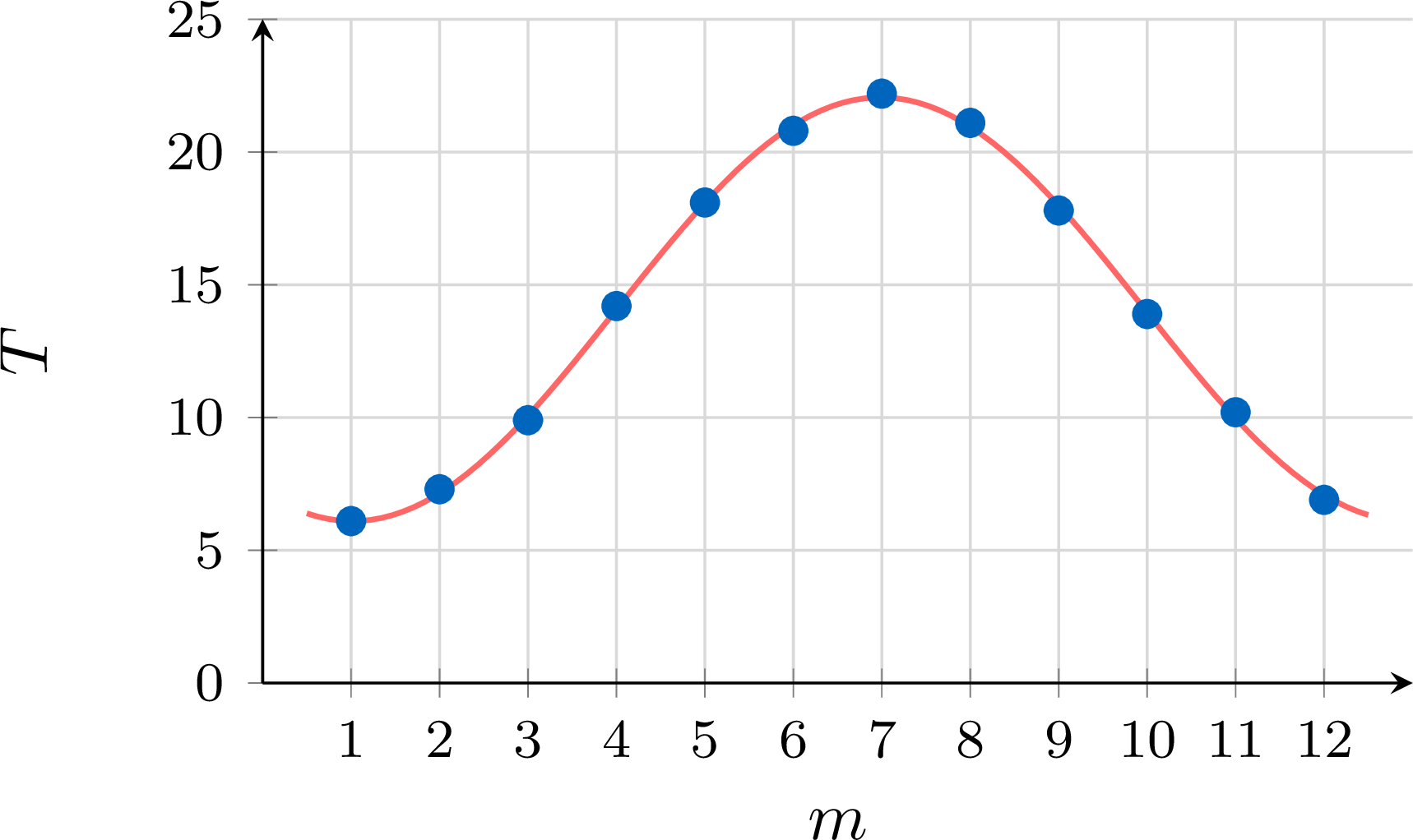
The mean temperature \(T\) of a city, in degrees Celsius, is recorded for each month \(m\), from \(m = 1\) (January) to \(m = 12\) (December). | \(m\) | \(1\) | \(2\) | \(3\) | \(4\) | \(5\) | \(6\) | \(7\) | \(8\) | \(9\) | \(10\) | \(11\) | \(12\) |
| \(T\) | \(6.1\) | \(7.3\) | \(9.9\) | \(14.2\) | \(18.1\) | \(20.8\) | \(22.2\) | \(21.1\) | \(17.8\) | \(13.9\) | \(10.2\) | \(6.9\) |
- Use technology to fit a model \(T = a\sin(bm + c) + d\), with the coefficients to \(3\) significant figures. Interpret \(b\) and \(d\).
- A model built by hand from the extreme values (amplitude and midline from the maximum and the minimum, period \(12\) months, maximum in July) is \(T = 8.05\sin\left(\frac{\pi}{6}(m - 4)\right) + 14.15\). Calculate the sum of square residuals of each model, to \(3\) decimal places. Which is the smaller, and why could this be expected?
- With \(m\) in L1 and \(T\) in L2, and the calculator in radians, the sine regression displays \(a = 7.980852865\), \(b = 0.526164882\), \(c = -2.105075244\) and \(d = 14.0797592\), and no coefficient of determination. So \(T \approx 7.98\sin(0.526m - 2.11) + 14.1\). (Some models display \(c + 2\pi \approx 4.18\) instead of \(c\), or a negative \(a\) with \(c\) shifted by \(\pi\): these give the same curve.) The period of the model is $$\begin{aligned}[t] \frac{2\pi}{b} &= \frac{2\pi}{0.52616\ldots} && \text{(period of a sine model)}\\ &\approx 11.9 \text{ months}, \end{aligned}$$ about one year, as expected for seasons; \(d \approx 14.1\) is the midline, the mean level around which the temperature oscillates, in degrees Celsius. Since \(bm + c = b\left(m + \frac{c}{b}\right)\) and \(-\frac{c}{b} \approx 4.0\), the model can also be written \(T \approx 7.98\sin\left(0.526(m - 4.0)\right) + 14.1\), very close to the model built by hand.
- With the unrounded coefficients of the sine regression, the residuals are, month by month, \(0.00\), \(0.15\), \(-0.17\), \(0.12\), \(0.01\), \(-0.21\), \(0.14\), \(0.15\), \(-0.18\), \(-0.06\), \(0.23\), \(-0.19\), and \(SS_{\text{res}} \approx 0.280\). For the model built by hand, the residuals are \(0.00\), \(0.12\), \(-0.23\), \(0.05\), \(-0.08\), \(-0.32\), \(0.00\), \(-0.02\), \(-0.38\), \(-0.25\), \(0.08\), \(-0.28\), and \(SS_{\text{res}} \approx 0.464\). The sine regression gives the smaller sum, as could be expected: it searches for the least squares curve among all the curves \(T = a\sin(bm + c) + d\) (drawn over the points, its curve follows them closely, a sign that the search has not stopped on a poorer curve), and the model built by hand is one of these curves, built from two values only (the maximum and the minimum).
Skills to practice
- Reading Regression Results
- Calculating the Sum of Square Residuals
- Fitting Regression Curves with Technology
- Choosing and Judging a Regression Model
V
Going further
Skills to practice
- Solving Problems with Changes of Variable
- Solving Problems with Regression Curves
- Quiz
Jump to section