International Baccalaureate · DP 1: Analysis and Approaches SL

Exponentials

⌚ ~186 min ▢ 21 blocks ✓ 93 exercises ➣ Prerequisites : Surds and Exponents, Sequences and Series, Functions, Transformations of functions

I Exponential Expressions and Equations

I.1 Rational Exponents

Recappreviously studied — click to reread

Discover

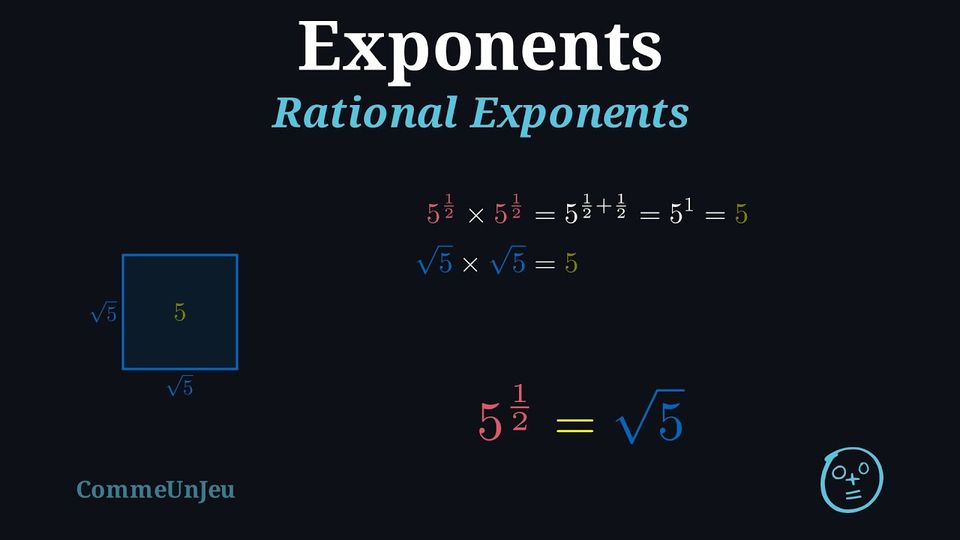
We know about positive exponents, like $5^3 = 5 \times 5 \times 5$, and also about negative exponents, like $5^{-3} = \dfrac{1}{5 \times 5 \times 5}$.
But what about fractional exponents?
Using the exponent laws, look at what happens with $\textcolor{colordef}{5^{\frac{1}{2}}}$:$$\begin{aligned}\textcolor{colordef}{5^{\frac{1}{2}}} \times \textcolor{colordef}{5^{\frac{1}{2}}} &= 5^{\frac{1}{2}+\frac{1}{2}} \\ &= 5^1 \\ &= \textcolor{olive}{5}\end{aligned}$$ And by the definition of the square root: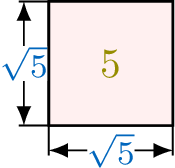

$$\textcolor{colorprop}{\sqrt{5}} \times \textcolor{colorprop}{\sqrt{5}} = \textcolor{olive}{5}$$ By comparing these two results, we see that:$$\textcolor{colordef}{5^{\frac{1}{2}}} \times \textcolor{colordef}{5^{\frac{1}{2}}} = \textcolor{colorprop}{\sqrt{5}} \times \textcolor{colorprop}{\sqrt{5}}$$ So, we can deduce that:$$\textcolor{colordef}{5^{\frac{1}{2}}} = \textcolor{colorprop}{\sqrt{5}}$$ Rational exponents are used only with positive bases, so that roots like $\sqrt[n]{a}$ are real numbers. This shows us that we can use fractional exponents to represent roots, extending our understanding of exponents to include rational exponents.

Definition — Rational Exponent

For a positive number $a$ and positive integers $m$ and $n$, $$\begin{aligned} a^{\frac{1}{2}} &= \sqrt{a}, \\ a^{\frac{1}{n}} &= \sqrt[n]{a}, \\ a^{\frac{m}{n}} &= \sqrt[n]{a^m} = \left(\sqrt[n]{a}\right)^m. \end{aligned}$$

For a positive base $a$, the exponent laws known for integer exponents remain true for rational exponents; they are used here without proof, as the opening problem of this section did with $5^{\frac{1}{2}} \times 5^{\frac{1}{2}} = 5^{\frac{1}{2} + \frac{1}{2}}$. In particular, $a^{-p} = \dfrac{1}{a^{p}}$ for every rational number $p$.

Report an error

Example

Without a calculator, evaluate:

$8^{\frac{2}{3}}$;
$16^{-\frac{3}{4}}$.

Answer

The definition gives two ways to write $a^{\frac{m}{n}}$. The form $\left(\sqrt[n]{a}\right)^m$ takes the root first, so the numbers stay small.

$$\begin{aligned}[t] 8^{\frac{2}{3}} &= \left(\sqrt[3]{8}\right)^2 && \text{(definition of a rational exponent)} \\ &= 2^2 && \text{(since } 2^3 = 8\text{)} \\ &= 4. \end{aligned}$$
$$\begin{aligned}[t] 16^{-\frac{3}{4}} &= \dfrac{1}{16^{\frac{3}{4}}} && \text{(negative exponent: } a^{-p} = \tfrac{1}{a^{p}}\text{)} \\ &= \dfrac{1}{\left(\sqrt[4]{16}\right)^3} && \text{(definition of a rational exponent)} \\ &= \dfrac{1}{2^3} && \text{(since } 2^4 = 16\text{)} \\ &= \dfrac{1}{8}. \end{aligned}$$

Taking the power first also works, but with larger numbers: $8^{\frac{2}{3}} = \sqrt[3]{8^2} = \sqrt[3]{64} = 4$.

Skills to practice

Evaluating Rational Powers without a Calculator
Simplifying Expressions with Rational Exponents

I.2 Exponential Expressions

Recappreviously studied — click to reread

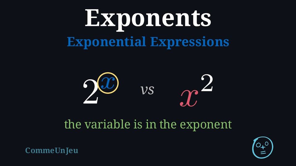
Definition — Exponential Expression

An exponential expression is a mathematical expression where a variable appears in the exponent.

Example

$2^x$ and $5^{x+1}$ are exponential expressions. This is different from a polynomial expression like $x^2$, where the variable is in the base.

Proposition — Algebraic Properties of $x \mapsto a^x$

Let $a \gt 0$. The rules of integer powers remain true for every real exponent; these properties are accepted without proof. For all real numbers $x$ and $y$ and every integer $n$:

$\textcolor{colorprop}{a^{x+y} = a^x \times a^y}$;
$\textcolor{colorprop}{a^{x-y} = \dfrac{a^x}{a^y}}$, and in particular $\textcolor{colorprop}{a^{-x} = \dfrac{1}{a^x}}$;
$\textcolor{colorprop}{a^{nx} = \left(a^x\right)^n}$.

They are used to transform numerical or literal expressions — the same gestures as with integer exponents.

Example

Write each expression as a single power, or as a number.

$2^{1.5} \times 2^{0.5}$
$\dfrac{5^{x+1}}{5^{x}}$
$\left(1.05^{x}\right)^{12}$
$\dfrac{1}{2^{x}}$

Answer

$\begin{aligned}[t]2^{1.5} \times 2^{0.5} &= 2^{1.5 + 0.5} &&\text{(product: add the exponents)}\\ &= 2^{2}\\ &= 4\end{aligned}$
$\begin{aligned}[t]\dfrac{5^{x+1}}{5^{x}} &= 5^{(x+1) - x} &&\text{(quotient: subtract the exponents)}\\ &= 5^{1}\\ &= 5\end{aligned}$
$\begin{aligned}[t]\left(1.05^{x}\right)^{12} &= 1.05^{12x} &&\text{(} a^{nx} = (a^x)^n \text{ with } n = 12\text{)}\end{aligned}$
$\begin{aligned}[t]\dfrac{1}{2^{x}} &= 2^{-x} &&\text{(} a^{-x} = \tfrac{1}{a^x}\text{)}\end{aligned}$

Method — Manipulating Exponential Expressions

Applying the exponent laws allows us to simplify, expand, and factorize complex expressions involving variables in the exponent. These skills are fundamental for solving exponential equations.

Example

Simplify $\frac{2^{x+1}+2^x}{2^x}$.

Answer

$$\begin{aligned}[t] \frac{2^{x+1}+2^x}{2^x} &= \frac{2^x \cdot 2^1 + 2^x}{2^x} && \scriptscriptstyle\text{(Using exponent law)} \\ &= \frac{2^x(2+1)}{2^x} && \scriptscriptstyle\text{(Factor out the common term } 2^x\scriptscriptstyle\text{)} \\ &= 3 && \scriptscriptstyle\text{(Cancel the common factor)} \end{aligned}$$

Skills to practice

Using the Laws with Real Exponents
Factorizing Exponential Expressions

I.3 The Number $e$

Discover

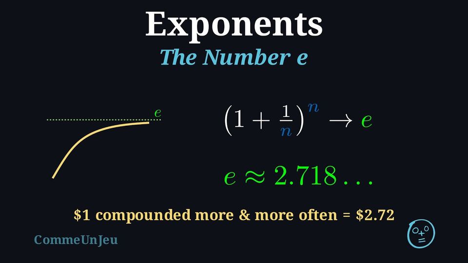
Let’s explore an idea from finance: compound interest.
Imagine you invest $\dollar 1$ in a special bank account that offers a $100\pourcent$ annual interest rate. We will see how much money you have after one year, depending on how often the interest is calculated (compounded) and added to your account.

Case 1: Compounded annually
The interest is paid once at the end of the year. The value is: $$ 1 \times (1 + 100\pourcent) = 1 \times (1+1) = \dollar 2. $$ So $$ \text{Value} = (1 + 1)^1. $$
Case 2: Compounded semi-annually
The interest is paid twice a year. The bank gives you half the annual rate ($50\pourcent$) each time.
- After 6 months: $1 \times \left(1 + \dfrac{1}{2}\right) = \dollar 1.50$
- At the end of the year: $1.50 \times \left(1 + \dfrac{1}{2}\right) = \dollar 2.25$
This can be calculated in one step as $$ 1 \times \left(1 + \frac{1}{2}\right)^2 = \dollar 2.25. $$ So $$ \text{Value} = \left(1 + \frac{1}{2}\right)^2. $$
Case $n$: Compounded $n$ times per year
If we compound $n$ times per year, the interest rate per period is $\dfrac{1}{n}$ (since the total annual rate is $100\pourcent$), and it is applied $n$ times. The value after one year is $$ \text{Value} = \left(1 + \frac{1}{n}\right)^n. $$

Let’s calculate the value of $\left(1 + \dfrac{1}{n}\right)^n$ for increasingly large values of $n$:

Compounding Frequency	$n$	Value $\left(1 + \dfrac{1}{n}\right)^n$
Annually	1	$(1 + 1/1)^1 = 2.00000$
Semi-annually	2	$(1 + 1/2)^2 = 2.25000$
Quarterly	4	$(1 + 1/4)^4 \approx 2.44141$
Monthly	12	$(1 + 1/12)^{12} \approx 2.61304$
Daily	365	$(1 + 1/365)^{365} \approx 2.71457$
Hourly	8,760	$(1 + 1/8760)^{8760} \approx 2.71813$

As you can see, the final amount increases, but it does not grow without bound. It seems to approach a specific number. This special irrational number is denoted by $e$, also known as Euler’s number. It represents the limiting value of this process of increasingly frequent compounding.

Definition — The Exponential Number $e$

The number e is defined as $$ e = \lim_{n\to\infty} \left(1 + \frac{1}{n}\right)^n. $$

Correct to five decimal places, $$ e \approx 2.71828\ldots $$ It is an irrational number, which means its decimal representation never terminates and never repeats.

Report an error

Skills to practice

Simplifying Powers of $e$
Simplifying Expressions in $e^x$
Expanding Expressions in $e^x$
Factorizing Expressions in $e^x$

I.4 Exponential Equations

Recappreviously studied — click to reread

Definition — Exponential Equation

An exponential equation is an equation in which the unknown occurs as part of the index or exponent.

Example

$2^x = 8$ and $30 \times 3^x = 7$ are both exponential equations.

There are a number of methods we can use to solve exponential equations. These include graphing, using technology, and by using logarithms, which we will study later. However, in some cases we can solve the equation algebraically by equating indices.

Report an error

Method — Solving by Equating Indices

For $a>0, a\neq 1$, $a^x = a^y$ if and only if $x = y$.

Example

Solve for $x$: $2^x = 16$

Answer

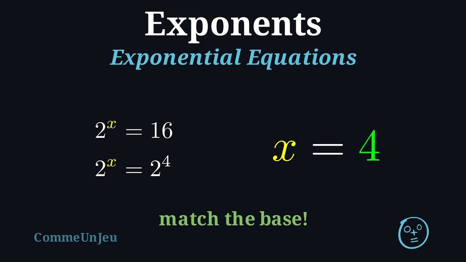
$$\begin{aligned}[t]\,&& 2^x &= 16 \\ \Leftrightarrow && 2^x &= 2^4 && \scriptscriptstyle\text{(Write 16 as a power of 2)} \\ \Leftrightarrow && x &= 4 && \scriptscriptstyle\text{(Equate the indices)}\end{aligned}$$

Skills to practice

Solving by Equating Indices

I.5 Equations in Quadratic Form

Method — Solving by Substitution

Some equations, while not quadratic in $x$, are quadratic in form. We can solve them by making a temporary substitution to create a standard quadratic equation.

Identify a substitution (e.g., let $u=x^2$ or $u=e^x$) that transforms the equation into the form $au^2+bu+c=0$.
Solve this new quadratic equation for $u$.
Substitute back to find the values for the original variable $x$. Remember to solve for all possible values of $x$.

Example

Solve the equation $x^4 - 5x^2 + 4 = 0$.

Answer

This equation is quadratic in $x^2$. Let $u = x^2$. Then $u^2 = (x^2)^2 = x^4$.

Substitute: The equation becomes: $$ u^2 - 5u + 4 = 0 $$
Solve for u: We can factorise this quadratic. $$ (u-1)(u-4) = 0 $$ So, $u=1$ or $u=4$.
Substitute back for x:
- If $u=1$, then $x^2=1 \implies x = \pm 1$.
- If $u=4$, then $x^2=4 \implies x = \pm 2$.

The four solutions are $x = -2, -1, 1, 2$.

Skills to practice

Solving Equations with $e$ and in Quadratic Form

II Exponential Functions

II.1 The Exponential Function $x \mapsto a^x$

Recappreviously studied — click to reread

Expressions like $a^n$ make sense when the exponent $n$ is an integer (roots give fractional exponents). The exponential function, written $f(x) = a^x$, extends that concept to any real exponent $x$.
This chapter presents the key features and graphs of these functions, and how they model real-world phenomena involving rapid growth or decay, such as population dynamics and compound interest.

Report an error

Definition — Exponential Function

The exponential function has the form $f(x)=a^x$, where the base $a$ is a positive constant and $a \neq 1$.

Proposition — Key Features of the Graph of $y\equal a^x$

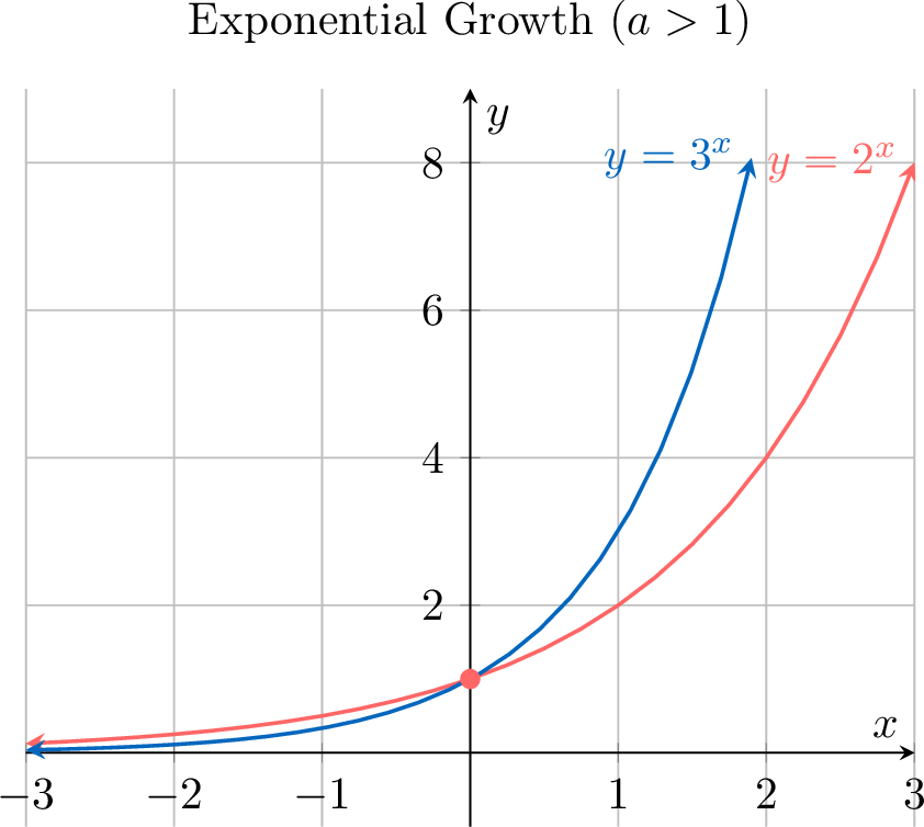
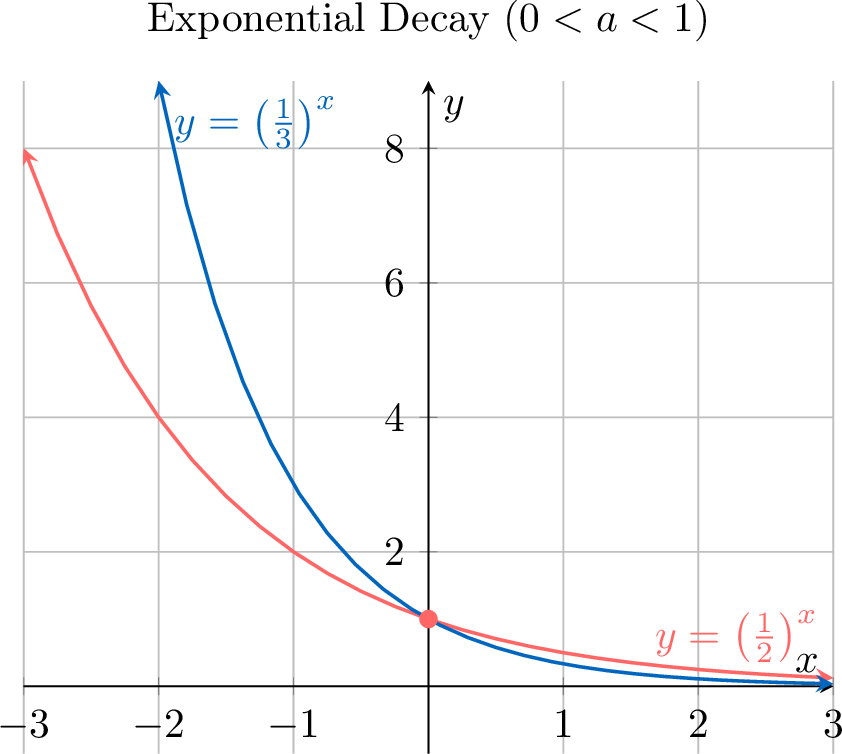
All exponential functions of the form $f(x) = a^x$ share several key graphical features:

Domain: The domain is all real numbers, $(-\infty, \infty)$.
Range: The range is all positive real numbers, $(0, \infty)$.
Horizontal Asymptote: The graph has a horizontal asymptote at the x-axis ($y=0$). The function approaches this line but never touches it.
y-intercept: The graph always passes through the point $(0, 1)$, because $a^0 = 1$ for any valid base $a$.
General Shape: The shape of the graph is determined by the value of the base, $a$:
- If $a > 1$, the function shows exponential growth and is increasing.
- If $0 < a < 1$, the function shows exponential decay and is decreasing.

$\quad$

Proposition — Variations of $x \mapsto k \times a^x$

Let $a \gt 0$ with $a \neq 1$, and let $k \neq 0$. The function $f$ defined for every real $x$ by $f(x) = k \times a^x$ satisfies $f(0) = k$ and has the sign of $k$.

If $\textcolor{colorprop}{k \gt 0}$, $f$ has the same variations as $x \mapsto a^x$: increasing if $a \gt 1$, decreasing if $0 \lt a \lt 1$.
If $\textcolor{colorprop}{k \lt 0}$, $f$ has the opposite variations: decreasing if $a \gt 1$, increasing if $0 \lt a \lt 1$.

(For $a = 1$ or $k = 0$, $f$ is constant.) Multiplying by a positive number keeps the order of two numbers; multiplying by a negative number reverses it. At the whole numbers $n = 0, 1, 2, \ldots$, the values $k \times a^n$ are multiplied by $a$ at each step: they form a geometric sequence, with first term $k$ and common ratio $a$, and the function and the sequence vary in the same way.

Example

Give the variations of each function on the set of real numbers.

$f(x) = 3 \times 1.2^{x}$
$g(x) = -2 \times 1.5^{x}$
$h(x) = 5 \times 0.8^{x}$
$m(x) = -0.5 \times 0.9^{x}$

Answer

$k = 3 \gt 0$ and $a = 1.2 \gt 1$: $f$ is increasing.
$k = -2 \lt 0$ and $a = 1.5 \gt 1$: $g$ is decreasing.
$k = 5 \gt 0$ and $0 \lt a = 0.8 \lt 1$: $h$ is decreasing.
$k = -0.5 \lt 0$ and $0 \lt a = 0.9 \lt 1$: $m$ is increasing — two reversals cancel out.

Skills to practice

Deciding the Variations of $x \mapsto k \times a^x$
Studying Exponential Functions

II.2 The Natural Exponential Function

Definition — Natural Exponential Function

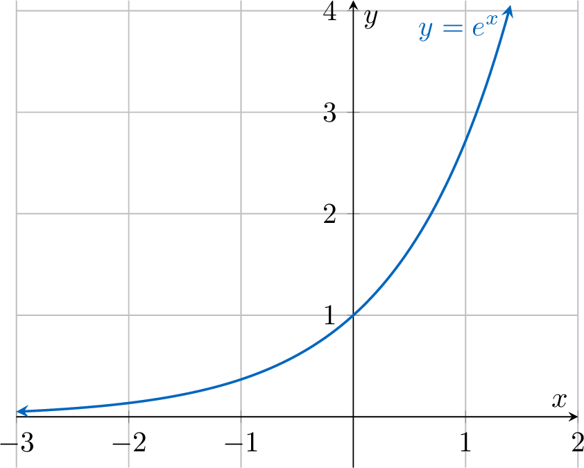
The natural exponential function is $x\mapsto e^x$.

Domain: $(-\infty, +\infty)$
Range: $(0, +\infty)$

Proposition — Graph and Properties of $y\equal e^x$

Horizontal Asymptote: The graph has a horizontal asymptote at the x-axis ($y=0$) as $x \to -\infty$.
y-intercept: The graph passes through the point $(0, 1)$, since $e^0 = 1$.
It is a strictly increasing function.

Skills to practice

Calculating with and Graphing $e^x$

II.3 Transformations of Exponential Functions

Recappreviously studied — click to reread

Proposition — Transformations of Exponential Functions

The graph of the general exponential function $f(x) = k \cdot a^{m(x-h)} + v$, with $a > 0$, $a \neq 1$, $k \neq 0$ and $m \neq 0$, can be obtained by applying transformations to the basic graph of $y=a^x$.

Vertical Translation ($v$): The graph is shifted vertically by $|v|$ units: up if $v > 0$, down if $v < 0$. The horizontal asymptote becomes $y=v$.
Horizontal Translation ($h$): The graph is shifted horizontally by $|h|$ units: to the right if $h > 0$, to the left if $h < 0$.
Vertical Stretch/Reflection ($k$): The graph is stretched vertically by a factor of $|k|$. If $k<0$, the graph is reflected in the horizontal asymptote.
Horizontal Stretch/Reflection ($m$): The graph is stretched horizontally by a factor of $1/|m|$ about the line $x=h$. If $m<0$, it is reflected in the vertical line $x=h$ (in the $y$-axis only when $h=0$).

Example

Sketch the graph of $f(x) = 2e^{-x} + 3$. State the domain, range, and equation of the asymptote.

Answer

The graph is a transformation of $y=e^x$: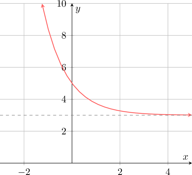

Reflection in the y-axis (due to the negative in front of $x$).
Vertical stretch by a factor of 2.
Vertical shift 3 units up.

The horizontal asymptote is $\boldsymbol{y=3}$.
The domain is $\boldsymbol{\mathbb{R}}$.
The range is $\boldsymbol{(3, \infty)}$.

Skills to practice

Describing Transformations of Exponential Graphs

III Growth and Decay

III.1 Exponential Models

Recappreviously studied — click to reread

Exponential functions are used to model quantities that change by a constant multiplicative factor over equal intervals of time. This core principle distinguishes them from linear functions, which change by a constant difference (addition or subtraction).
There are two main types of exponential models:

Exponential Growth: The quantity increases by a constant factor greater than 1. This is seen in phenomena like population growth and compound interest.
Exponential Decay: The quantity decreases by a constant factor between 0 and 1. This is seen in phenomena like radioactive decay and asset depreciation.

These models can be discrete, occurring in distinct steps (e.g., interest compounded annually), or continuous, occurring smoothly over time (e.g., bacterial growth).

Report an error

Definition — General Model for Exponential Growth and Decay

An exponential relationship is described by the function:$$ A(t) = A_0 \times R^t $$ where:

$A(t)$ is the amount at time $t$.
$A_0$ is the initial amount (the amount at $t=0$).
$R$ is the constant growth or decay factor per unit of time, with $R > 0$: $R = 1 + r$ for a growth at the rate $r$, $R = 1 - r$ for a decay at the rate $r$.
$t$ is the time elapsed.

The function $A(t) = A_0 \times R^t$ is a function $k \times a^x$, with $k = A_0$ and $a = R$.

Example

The population of foxes, $P$, in a specified area, $t$ years after observation began, is modelled by the equation: $P(t)=300(1.25)^t$.

How many foxes are there initially?
What is the annual percentage growth rate?
How many foxes are there after 5 years?

Answer

The initial population corresponds to $t=0$. $$P(0) = 300(1.25)^0 = 300 \times 1 = \boldsymbol{300} \text{ foxes}$$
The growth factor is $R=1.25$. Since $R = 1+r$, we have $1.25 = 1+r$, which gives $r=0.25$.
The annual growth rate is $\boldsymbol{25\pourcent}$.
Substitute $t=5$ into the equation. Since the population must be a whole number, we round to the nearest fox. $$P(5) = 300(1.25)^5 \approx 915.52... \approx \boldsymbol{916} \text{ foxes}$$

Example

An amount of $\dollar 5\,000$ is invested at $6\pourcent$ p.a. compounded annually.

Find a model for the amount, $A$, after $t$ years.
Find the amount after 4 years.

Answer

The initial amount is $A_0 = 5\,000$. The annual interest rate is $r = 0.06$.
The growth factor is $R = 1+r = 1+0.06 = 1.06$.
The model is $\boldsymbol{A(t) = 5\,000(1.06)^t}$.
After 4 years, the amount is: $$A(4) = 5\,000(1.06)^4 \approx 6\,312.38...$$ The amount is $\boldsymbol{\dollar 6\,312.38}$.

Skills to practice

Modelling Growth and Decay

III.2 Solving Exponential Equations with Technology

Equating exponents solves $2^x = 16$, because both sides are powers of $2$. The equation $3^x = 7$ cannot be solved this way: $7$ is not a power of $3$ with a whole-number exponent. Comparing with the powers of $3$ still locates its solution: $$3^1 = 3 < 7 < 9 = 3^2,$$ so the solution lies between $1$ and $2$. Its value is read on the graphs of $y = 3^x$ and $y = 7$, with technology. Two questions come first: is there always a solution, and can there be more than one?

Report an error

Proposition — Number of Solutions of an Exponential Equation

Let $a > 0$ with $a \neq 1$, and let $k$ be a real number. The equation $a^x = k$ has

exactly one solution if $k > 0$;
no solution if $k \leq 0$.

Proof

The key features of the graph of $y = a^x$, stated with the exponential functions (domain: all real numbers; range: the positive numbers; increasing if $a > 1$, decreasing if $0 < a < 1$), give the two cases.

If $k \leq 0$: the range of $x \mapsto a^x$ is the set of positive numbers, so $a^x > 0 \geq k$ for every $x$, and the equation has no solution.
If $k > 0$: $k$ belongs to the range, so at least one number $x$ satisfies $a^x = k$. There is only one: if $a^x = k$ and $a^y = k$, then $a^x = a^y$, hence $x = y$ by the method of equating exponents. Graphically, the horizontal line $y = k$ meets the graph once, since the graph is increasing when $a > 1$ and decreasing when $0 < a < 1$.

Method — Solving an Exponential Equation with Technology

To solve an equation such as $a^x = k$, or $c \times a^x = k$ with $c \neq 0$:

Count the solutions: isolate the power, $a^x = \dfrac{k}{c}$, and apply the proposition “Number of Solutions of an Exponential Equation”. If the right side is not positive, there is no solution and nothing to graph.
Locate the solution between two consecutive integers by comparing with the powers of $a$ (a table of values does it). If the right side is itself a power of $a$ with an integer exponent, that integer is the exact solution, found by equating exponents. The two integers give the $x$-range of the window; its $y$-range must contain the right side.
Enter each side as a function, $Y_1$ = left side and $Y_2$ = right side, graph them, and choose intersection in the analysis tools of the graph menu. The solution is the $x$-coordinate $X$ of the point displayed; its $y$-coordinate is the common value of the two sides.
Round as the question asks (to 3 significant figures if it says nothing), then check: the left side, evaluated at the rounded value, is close to the right side.

The equation solver of a calculator, given a first guess inside the interval of step 2, returns the same value.

Example

Solve each equation, with technology where it is needed. Give each solution to 3 significant figures.

$2^x = 12$;
$4 \times 0.8^x = 1.5$;
$5 \times 2^x = -10$.

Answer

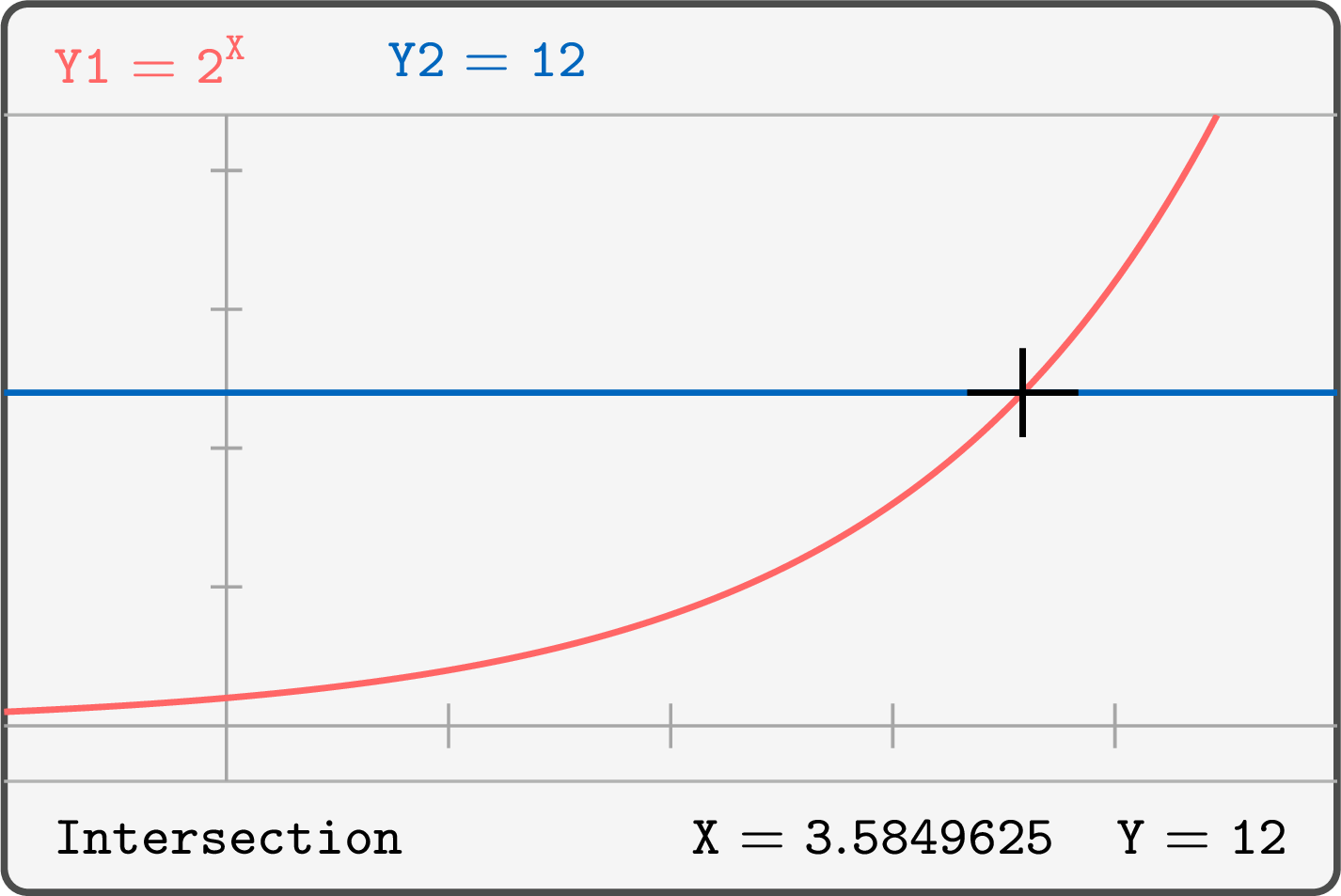
Since $12 > 0$, the equation has exactly one solution, and $2^3 = 8 < 12 < 16 = 2^4$ places it between $3$ and $4$. The two sides are entered as $Y_1 = 2^x$ and $Y_2 = 12$, and graphed in the window $-1 \le x \le 5$, $-2 \le y \le 22$. The intersection tool displays $X = 3.5849625$ and $Y = 12$. The solution is $x \approx 3.58$. Check: $2^{3.58} \approx 11.96$, close to $12$; the small gap comes from the rounding.
First the power is isolated: $$\begin{aligned}[t] 4 \times 0.8^x &= 1.5 \\ 0.8^x &= 0.375. && \text{(divide both sides by } 4\text{)} \end{aligned}$$ Since $0.375 > 0$, there is exactly one solution. The base $0.8$ is less than $1$, so the powers decrease: $0.8^4 = 0.4096 > 0.375 > 0.32768 = 0.8^5$, and the solution lies between $4$ and $5$. With $Y_1 = 4 \times 0.8^x$ and $Y_2 = 1.5$, in the window $0 \le x \le 8$, $0 \le y \le 5$, the intersection tool displays $X = 4.3955079$. The solution is $x \approx 4.40$, the final zero being the third significant figure. Check: $4 \times 0.8^{4.40} \approx 1.498$, close to $1.5$.
The power is isolated first: $$\begin{aligned}[t] 5 \times 2^x &= -10 \\ 2^x &= -2. && \text{(divide both sides by } 5\text{)} \end{aligned}$$ The right side is negative, and $2^x > 0$ for every $x$: the equation has no solution, and there is nothing to graph.

Definition — Half-Life

For a quantity that decreases according to $A(t) = A_0 \times b^t$, with $A_0 > 0$ and $0 < b < 1$, the half-life is the time $T$ after which the quantity is halved: $$A(T) = \dfrac{A_0}{2}, \quad \text{that is} \quad b^T = \dfrac{1}{2}.$$

Example

A patient is given $400$ mg of a medicine. The amount left in the body $t$ hours later is modelled by $A(t) = 400 \times 0.82^t$ mg.

Find the half-life of the medicine, to 3 significant figures.
The medicine no longer acts below $50$ mg. After how many whole hours is the amount first below $50$ mg?

Answer

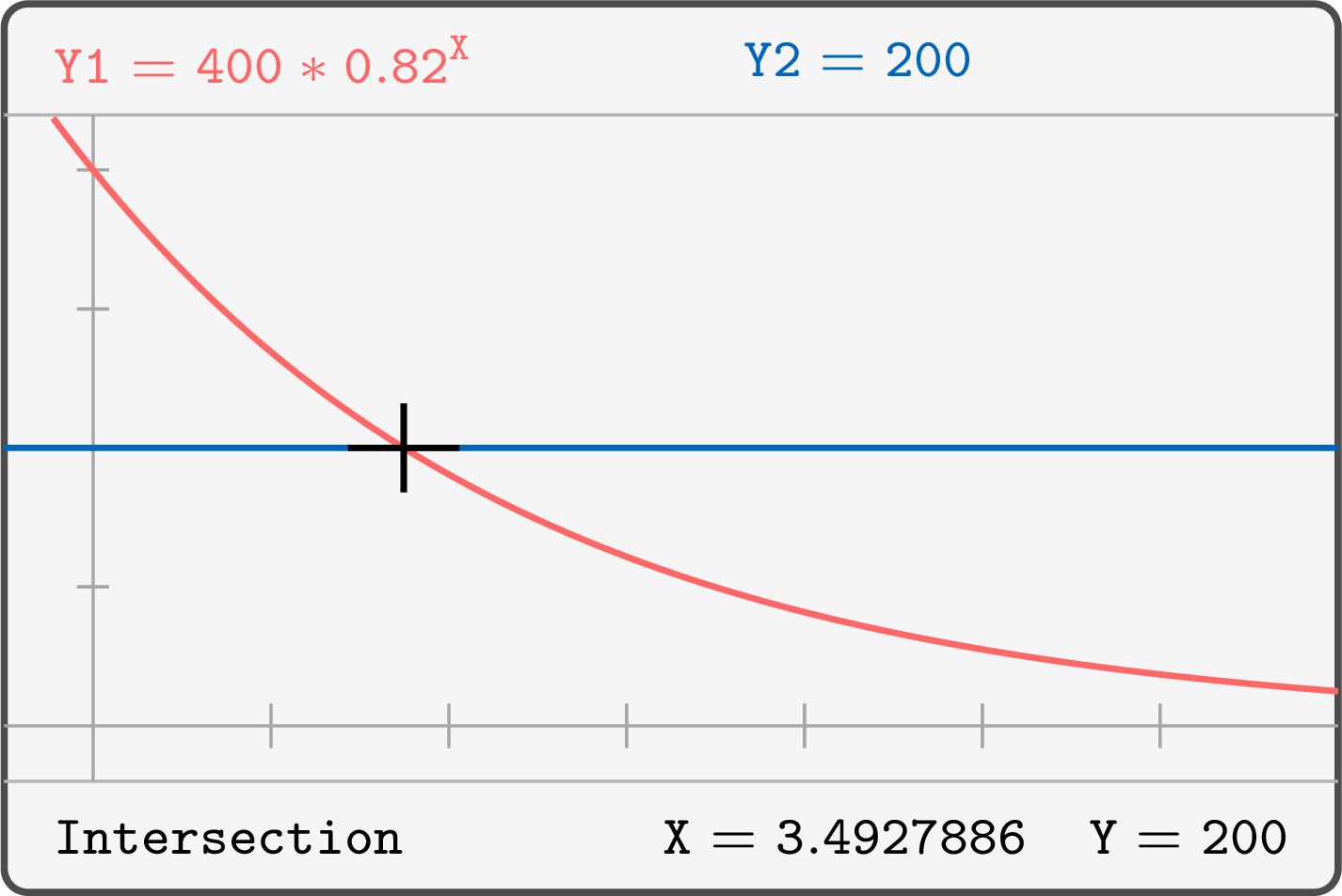
The half-life $T$ satisfies $A(T) = 200$: $$\begin{aligned}[t] 400 \times 0.82^T &= 200 \\ 0.82^T &= 0.5. && \text{(divide both sides by } 400\text{)} \end{aligned}$$ Since $0.5 > 0$, there is exactly one solution. With $Y_1 = 400 \times 0.82^x$ and $Y_2 = 200$, in the window $-1 \le x \le 14$, $-40 \le y \le 440$, the intersection tool displays $X = 3.4927886$. The half-life is $T \approx 3.49$ hours. Check: $400 \times 0.82^{3.49} \approx 200.1$. The equation $0.82^T = 0.5$ does not involve the initial dose: the half-life would be the same for any dose.
The base $0.82$ is less than $1$, so the amount decreases, and it is enough to find the first whole hour at which it is below $50$ mg. A table of values of $Y_1$ at whole numbers gives:

$t$ (h) $9$ $10$ $11$ $12$

$A(t)$ (mg) $67.05$ $54.98$ $45.08$ $36.97$

$A(10) \approx 54.98 > 50$ and $A(11) \approx 45.08 < 50$: the amount is first below $50$ mg after $11$ hours.
Check with the half-life: $50 = \dfrac{400}{8}$, three halvings, so the amount reaches $50$ mg after $3 \times 3.49 \approx 10.5$ hours, between $10$ and $11$.

Skills to practice

Counting and Locating Solutions
Solving Equations with the Intersection Tool
Finding When a Model Reaches a Value
Writing Up a Solution Found with Technology

IV Going further

Skills to practice

Solving Problems without Technology
Solving Problems with Technology
Quiz

\(t\) (h)	\(9\)	\(10\)	\(11\)	\(12\)
\(A(t)\) (mg)	\(67.05\)	\(54.98\)	\(45.08\)	\(36.97\)

Compounding Frequency	\(n\)	Value \(\left(1 + \dfrac{1}{n}\right)^n\)
Annually	1	\((1 + 1/1)^1 = 2.00000\)
Semi-annually	2	\((1 + 1/2)^2 = 2.25000\)
Quarterly	4	\((1 + 1/4)^4 \approx 2.44141\)
Monthly	12	\((1 + 1/12)^{12} \approx 2.61304\)
Daily	365	\((1 + 1/365)^{365} \approx 2.71457\)
Hourly	8,760	\((1 + 1/8760)^{8760} \approx 2.71813\)