International Baccalaureate · DP 2: Applications and Interpretation SL
Properties of Curves
I
Tangents and Normals
I.1
Equation of the Tangent
The most direct geometric interpretation of the derivative is that it gives the gradient (also called slope) of the tangent line. Finding the equation of this line is a fundamental application of differentiation.
Proposition — Equation of the Tangent
Assume \(f\) is differentiable at \(x=a\) and that the tangent is not vertical. Then the equation of the tangent to the curve \(y=f(x)\) at the point \((a, f(a))\) is:$$\textcolor{colorprop}{y = f^{\prime}(a)(x-a) +f(a)}$$ 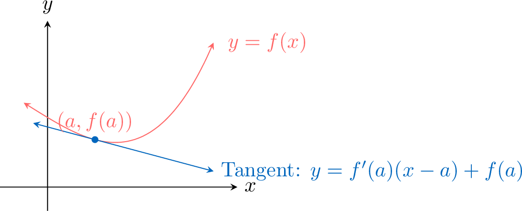
Let \(B(x,y)\) be any point on the tangent line. The point of tangency is \(A(a,f(a))\), which also belongs to the tangent line.
The gradient of a line is given by the formula \(m = \dfrac{\Delta y}{\Delta x}\). Using points \(A\) and \(B\), the gradient of the tangent line is:$$ m = \dfrac{y-f(a)}{x-a}\quad \text{for }x\neq a. $$ By definition, the gradient of the tangent to the curve \(y=f(x)\) at the point \(x=a\) is the value of the derivative at that point, so:$$ m = f'(a). $$ Equating the two expressions for the gradient, we get:$$ f'(a) = \dfrac{y-f(a)}{x-a}. $$ Multiplying both sides by \((x-a)\) gives the point-gradient form of the equation:$$ y - f(a) = f'(a)(x-a). $$ Making \(y\) the subject gives:$$ y = f'(a)(x-a) + f(a). $$
The gradient of a line is given by the formula \(m = \dfrac{\Delta y}{\Delta x}\). Using points \(A\) and \(B\), the gradient of the tangent line is:$$ m = \dfrac{y-f(a)}{x-a}\quad \text{for }x\neq a. $$ By definition, the gradient of the tangent to the curve \(y=f(x)\) at the point \(x=a\) is the value of the derivative at that point, so:$$ m = f'(a). $$ Equating the two expressions for the gradient, we get:$$ f'(a) = \dfrac{y-f(a)}{x-a}. $$ Multiplying both sides by \((x-a)\) gives the point-gradient form of the equation:$$ y - f(a) = f'(a)(x-a). $$ Making \(y\) the subject gives:$$ y = f'(a)(x-a) + f(a). $$
Example
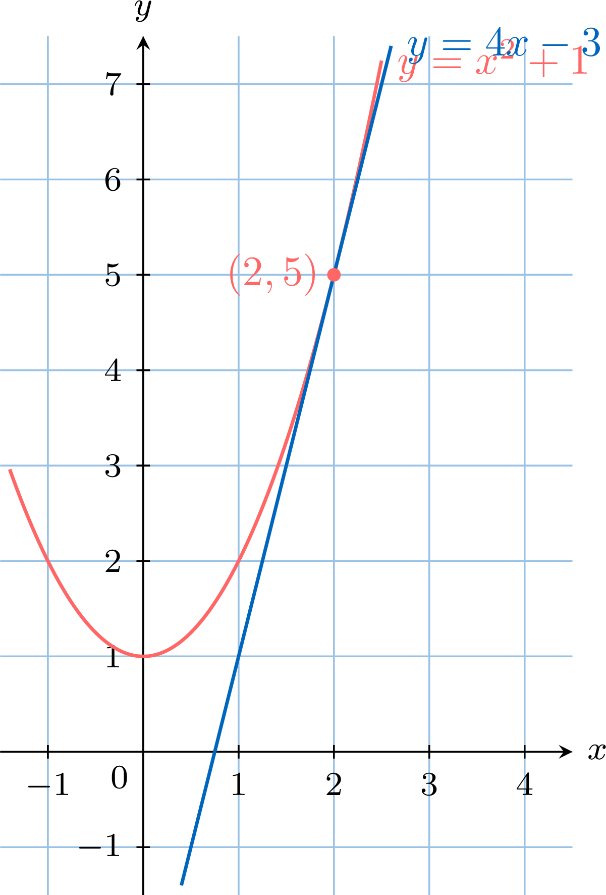
Let \(f(x) = x^2 + 1\). - Using the definition of the derivative, compute \(f'(2)\).
- Deduce the equation of the tangent to the curve of \(f\) at the point with \(x\)-coordinate \(2\).
- \(f(2) = 5\) and \(f(2+h) = (2+h)^2 + 1 = 5 + 4h + h^2\). For \(h \neq 0\), $$ \dfrac{f(2+h)-f(2)}{h} = \dfrac{4h + h^2}{h} = 4 + h \xrightarrow[h \to 0]{} 4. $$ So \(f'(2) = 4\).
- The tangent passes through the point \((2, f(2)) = (2, 5)\) with gradient \(f'(2) = 4\): $$ y = f'(2)(x - 2) + f(2) = 4(x-2) + 5 = 4x - 3. $$
Method — Constructing a Tangent from the Derivative
To draw the tangent to the curve of \(f\) at the point \(A(a, f(a))\) when the number \(f'(a)\) is known: - Place the point \(A\) on the curve.
- Use the gradient \(f'(a)\) to find a second point: from \(A\), move \(1\) unit to the right and \(f'(a)\) units up (down if \(f'(a) < 0\)). If \(f'(a) = \dfrac{p}{q}\) is a fraction, move \(q\) units to the right and \(p\) units up instead.
- Draw the line through \(A\) and this second point: it is the tangent.
Example
The curve of a function \(f\) is drawn below. We know that \(f(1) = 2\) and \(f'(1) = -\dfrac{1}{2}\). Construct the tangent to the curve at the point with \(x\)-coordinate \(1\). 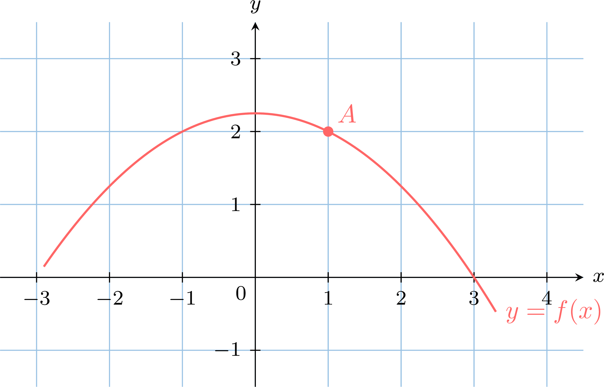
The tangent passes through \(A(1, 2)\) with gradient \(f'(1) = -\dfrac{1}{2}\): from \(A\), we move \(2\) units to the right and \(1\) unit down, which gives the second point \(B(3, 1)\). The tangent is the line \(AB\). 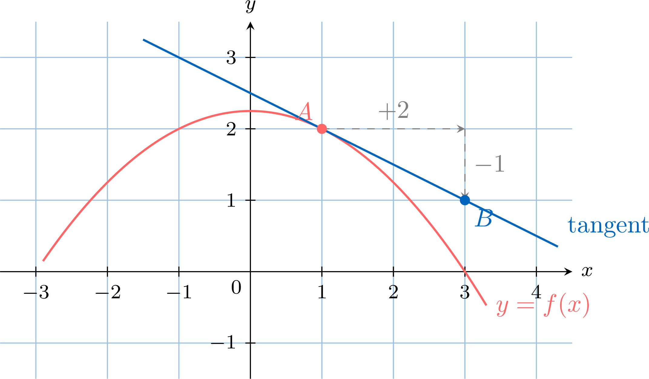
Check: the line \(AB\) has equation \(y = -\dfrac{1}{2}(x-1) + 2 = -\dfrac{1}{2}x + \dfrac{5}{2}\), which is indeed \(y = f'(1)(x-1) + f(1)\).
Example
Let \(f(x) = x^3 + 3x^2 - 1\). - Determine the points of the curve of \(f\) where the tangent is parallel to the line \(y = 9x + 4\), and give the equation of each of these tangents.
- Determine the points of the curve where the tangent is horizontal.
\(f'(x) = 3x^2 + 6x\). Two parallel lines have the same gradient: the tangent at the point with \(x\)-coordinate \(a\) is parallel to the line \(y = 9x + 4\) when its gradient \(f'(a)\) equals \(9\). 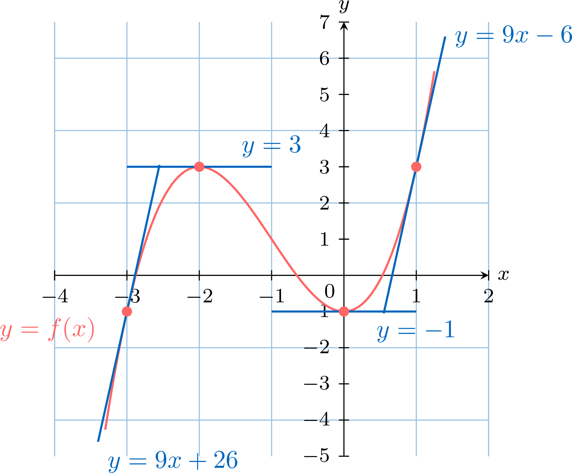
- We solve \(f'(x) = 9\): $$\begin{aligned}[t] 3x^2 + 6x &= 9 \\ x^2 + 2x - 3 &= 0 &&\text{(subtract } 9 \text{, divide by } 3\text{)} \\ (x - 1)(x + 3) &= 0, &&\text{(factorise)} \end{aligned}$$ so \(x = 1\) or \(x = -3\): there are two such points. At \(x = 1\), \(f(1) = 1 + 3 - 1 = 3\) and $$\begin{aligned}[t] y &= f'(1)(x - 1) + f(1) &&\text{(equation of the tangent)} \\ &= 9(x - 1) + 3 \\ &= 9x - 6. \end{aligned}$$ At \(x = -3\), \(f(-3) = -27 + 27 - 1 = -1\) and $$\begin{aligned}[t] y &= f'(-3)(x + 3) + f(-3) &&\text{(equation of the tangent)} \\ &= 9(x + 3) - 1 \\ &= 9x + 26. \end{aligned}$$ The tangents at \((1, 3)\) and at \((-3, -1)\) are both parallel to the line \(y = 9x + 4\).
- A horizontal tangent has gradient \(0\), so we solve \(f'(x) = 0\): $$\begin{aligned}[t] 3x^2 + 6x &= 0 \\ 3x(x + 2) &= 0, &&\text{(factorise)} \end{aligned}$$ so \(x = 0\) or \(x = -2\), with \(f(0) = -1\) and \(f(-2) = -8 + 12 - 1 = 3\). The tangent is horizontal at \((0, -1)\), with equation \(y = -1\), and at \((-2, 3)\), with equation \(y = 3\).
Proposition — Where a Tangent Crosses the \(x\)-Axis
Let \(f\) be differentiable at \(a\), with \(f'(a) \neq 0\). The tangent to the curve of \(f\) at the point with \(x\)-coordinate \(a\) crosses the \(x\)-axis at the point with \(x\)-coordinate $$a - \dfrac{f(a)}{f'(a)}.$$
The tangent has equation \(y = f'(a)(x - a) + f(a)\). A point of this line lies on the \(x\)-axis when \(y = 0\): \begin{align*} f'(a)(x - a) + f(a) = 0 &\iff f'(a)(x - a) = -f(a)
&\iff x - a = -\dfrac{f(a)}{f'(a)} && \text{(division by } f'(a) \neq 0\text{)}
&\iff x = a - \dfrac{f(a)}{f'(a)}. \end{align*} When \(f'(a) = 0\), the division cannot be made: the tangent is horizontal (it is the \(x\)-axis itself when \(f(a) = 0\)).
&\iff x - a = -\dfrac{f(a)}{f'(a)} && \text{(division by } f'(a) \neq 0\text{)}
&\iff x = a - \dfrac{f(a)}{f'(a)}. \end{align*} When \(f'(a) = 0\), the division cannot be made: the tangent is horizontal (it is the \(x\)-axis itself when \(f(a) = 0\)).
Example
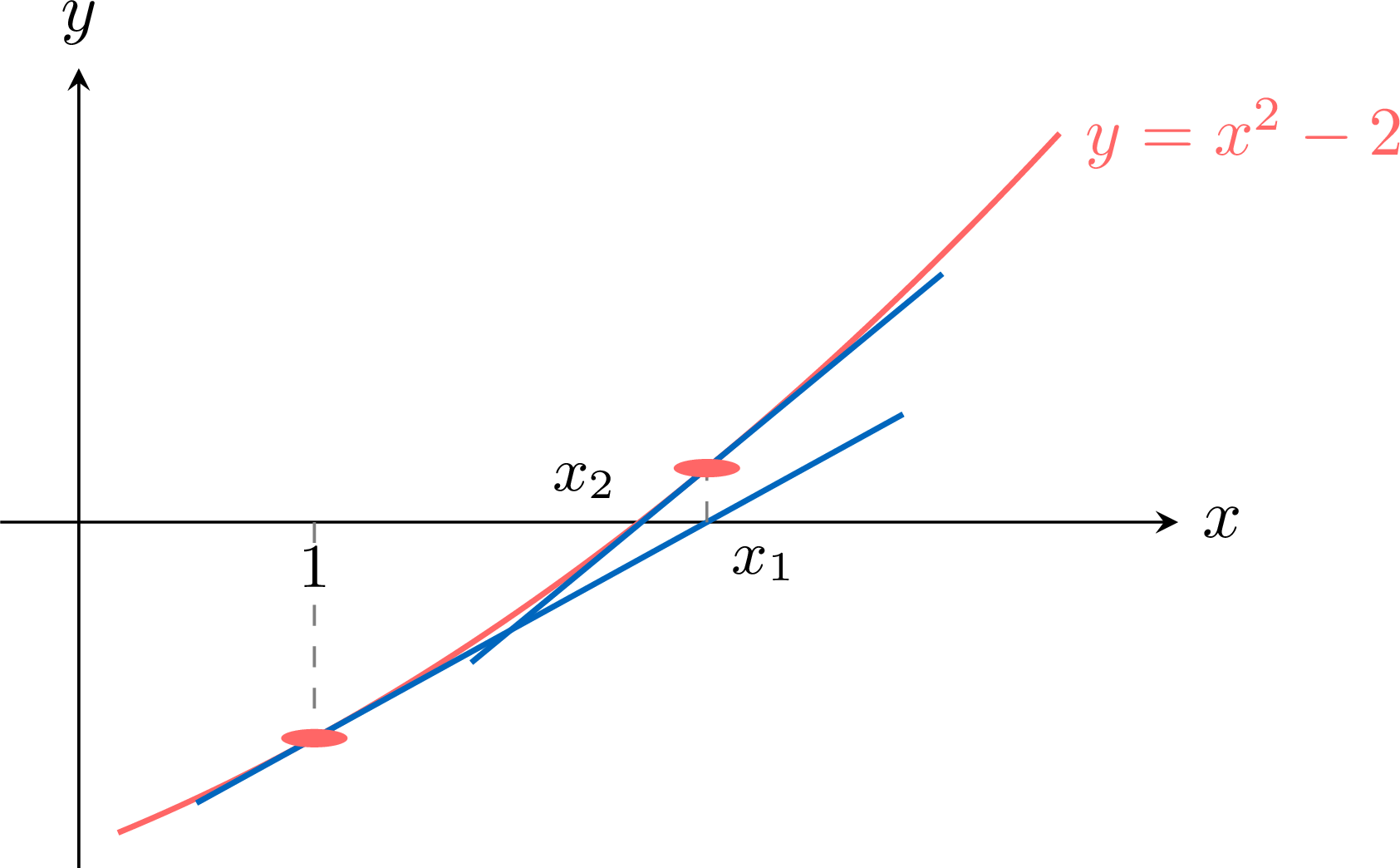
The function \(f\) is defined on \(\mathbb{R}\) by \(f(x) = x^2 - 2\). Its curve crosses the \(x\)-axis at \(-\sqrt{2}\) and at \(\sqrt{2}\); the positive one, \(\sqrt{2}\), is a number no decimal writes exactly. - Determine the \(x\)-coordinate \(x_1\) of the point where the tangent at the point with \(x\)-coordinate \(1\) crosses the \(x\)-axis.
- Determine the \(x\)-coordinate \(x_2\) of the point where the tangent at the point with \(x\)-coordinate \(x_1\) crosses the \(x\)-axis.
- Compare \(1\), \(x_1\) and \(x_2\) with \(\sqrt{2} \approx 1.41421\).
- \(f'(x) = 2x\), so \(f(1) = -1\) and \(f'(1) = 2 \neq 0\). The formula \(a - \dfrac{f(a)}{f'(a)}\) with \(a = 1\) gives \(x_1 = 1 - \dfrac{-1}{2} = \dfrac{3}{2}\).
- \(f\left(\dfrac{3}{2}\right) = \dfrac{9}{4} - 2 = \dfrac{1}{4}\) and \(f'\left(\dfrac{3}{2}\right) = 3\), so $$x_2 = \dfrac{3}{2} - \dfrac{1/4}{3} = \dfrac{3}{2} - \dfrac{1}{12} = \dfrac{17}{12} \approx 1.41667.$$
- The distance to \(\sqrt{2}\) is about \(0.414\) for \(1\), \(0.086\) for \(x_1\), and \(0.0025\) for \(x_2\): each tangent gives a value much closer to \(\sqrt{2}\) than the point it starts from.
Skills to practice
- Finding the Equation of a Tangent
- Finding Tangents at a Point or with a Given Gradient
I.2
The Tangent with Technology
Method — Finding the Equation of a Tangent with Technology
To find the equation of the tangent to the curve of \(f\) at the point where \(x = a\), with a graphing calculator: - Compute \(f(a)\), by substitution or with the value tool of the graph menu.
- Compute \(f'(a)\) with the derivative command, \(f\) being differentiable at \(a\), and store the full value in a memory of the calculator.
- Write the equation \(y = f'(a)(x - a) + f(a)\) and expand it to the form \(y = mx + c\) with the stored value. Round \(m\) and \(c\) only at the end, to 3 significant figures: rounding \(f'(a)\) first changes \(c\).
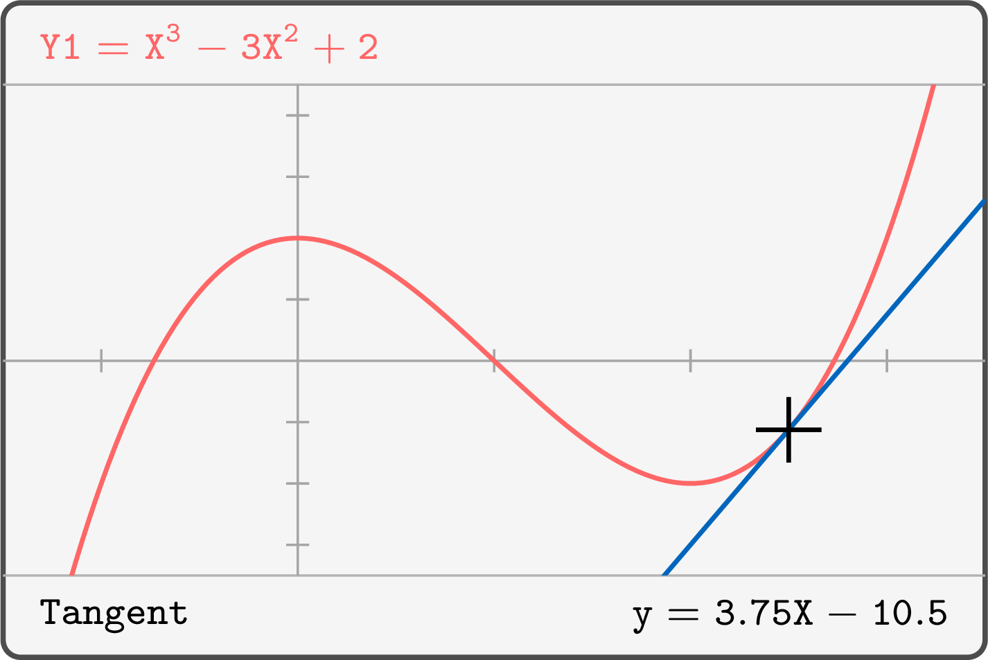
- Check on the screen: the tangent tool of the graph menu (draw or sketch menu, depending on the model), at \(x = a\), draws the tangent and displays its equation. The line must touch the curve at the point \((a, f(a))\), and its equation must match the one found.
Example
Let \(f(x) = 2^x\). Use technology to find the equation of the tangent to the curve of \(f\) at the point where \(x = 1\), in the form \(y = mx + c\) with \(m\) and \(c\) to 3 significant figures.
The point. \(f(1) = 2^1 = 2\): the point of tangency is \((1, 2)\).
The gradient. \(f\) is an exponential function, differentiable at every real number. The derivative command, with \(2^X\) and \(X = 1\), displays \(1.386294361\), stored in a memory.
The equation. $$\begin{aligned}[t] y &= f'(1)(x - 1) + f(1) &&\text{(equation of the tangent)} \\ &\approx 1.386294361(x - 1) + 2 \\ &\approx 1.386294361x + 0.613705639. &&\text{(expand)} \end{aligned}$$ Rounded at the end: \(y \approx 1.39x + 0.614\). Rounding the gradient first would give \(2 - 1.39 = 0.61\), a wrong constant. The tangent tool at \(X = 1\) draws the line through \((1, 2)\) and displays the same coefficients before rounding. 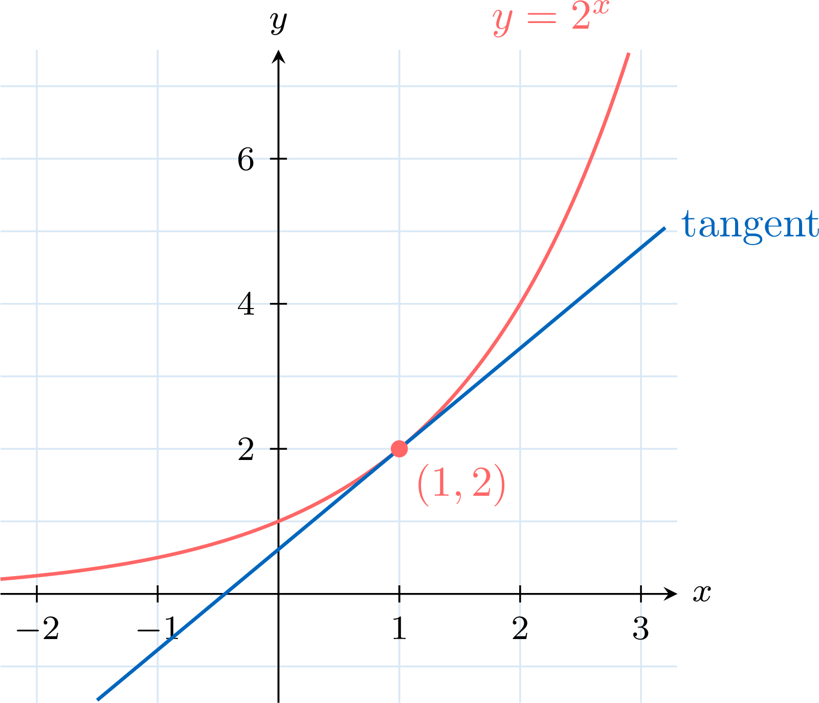
The gradient. \(f\) is an exponential function, differentiable at every real number. The derivative command, with \(2^X\) and \(X = 1\), displays \(1.386294361\), stored in a memory.
The equation. $$\begin{aligned}[t] y &= f'(1)(x - 1) + f(1) &&\text{(equation of the tangent)} \\ &\approx 1.386294361(x - 1) + 2 \\ &\approx 1.386294361x + 0.613705639. &&\text{(expand)} \end{aligned}$$ Rounded at the end: \(y \approx 1.39x + 0.614\). Rounding the gradient first would give \(2 - 1.39 = 0.61\), a wrong constant. The tangent tool at \(X = 1\) draws the line through \((1, 2)\) and displays the same coefficients before rounding.
Skills to practice
- Finding a Tangent with Technology
I.3
Equation of the Normal
Definition — Normal Line
The normal line to a curve at a point is the line that is perpendicular to the tangent line at that same point. 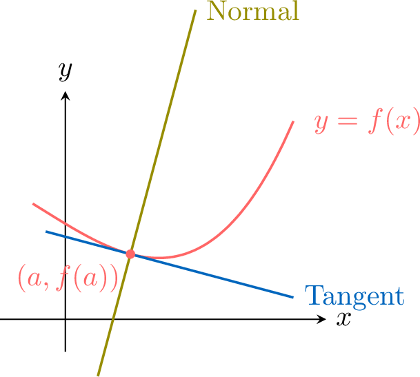
Proposition — Equation of the Normal
The equation of the normal to the curve \(y=f(x)\) at the point \((a, f(a))\) is given by: - if \(f'(a)\neq 0\), then the normal has gradient \(-\dfrac{1}{f'(a)}\) and $$\textcolor{colorprop}{y = -\frac{1}{f'(a)}(x-a)+f(a)}.$$
- if \(f'(a)= 0\), then the tangent is horizontal and the normal is the vertical line \(x=a\).
- if the tangent is vertical (so its equation is \(x=a\)), then the normal is the horizontal line \(y=f(a)\).
The gradient of the tangent at \(x=a\) is \(m_T = f'(a)\). Because the normal line is perpendicular to the tangent line, its gradient \(m_N\) is the negative reciprocal of the tangent's gradient:$$ m_N = -\frac{1}{m_T} = -\frac{1}{f'(a)} \quad (\text{provided } f'(a) \neq 0). $$ Using the point-gradient form of a line with the point \((a, f(a))\) and the gradient \(m_N\), we get the equation of the normal:$$ y - f(a) = -\frac{1}{f'(a)}(x-a). $$ The special cases \(f'(a)=0\) (horizontal tangent) and vertical tangent are handled as described in the statement above.
Example
Let \(f(x) = 3^x\). Use technology to find the equation of the normal to the curve of \(f\) at the point where \(x = 1\), in the form \(y = mx + c\) with \(m\) and \(c\) to 3 significant figures.
The point. \(f(1) = 3^1 = 3\): the point is \((1, 3)\).
The gradient of the tangent. The derivative command, with \(3^X\) and \(X = 1\), displays about \(3.29584\) (the last digits depend on the model), kept in a memory. It is not zero, so the normal is not vertical, and its gradient is $$-\frac{1}{f'(1)} \approx -0.30341.$$ The equation of the normal. $$\begin{aligned}[t] y &= -\frac{1}{f'(1)}(x - 1) + f(1) &&\text{(equation of the normal)} \\ &\approx -0.30341(x - 1) + 3 \\ &\approx -0.30341x + 3.30341. &&\text{(expand)} \end{aligned}$$ Rounded at the end: \(y \approx -0.303x + 3.30\). Some calculators draw the normal directly (normal tool of the sketch menu) and display its equation: a check. On the screen, as on the figure, the normal looks perpendicular to the tangent only when both axes have the same unit. 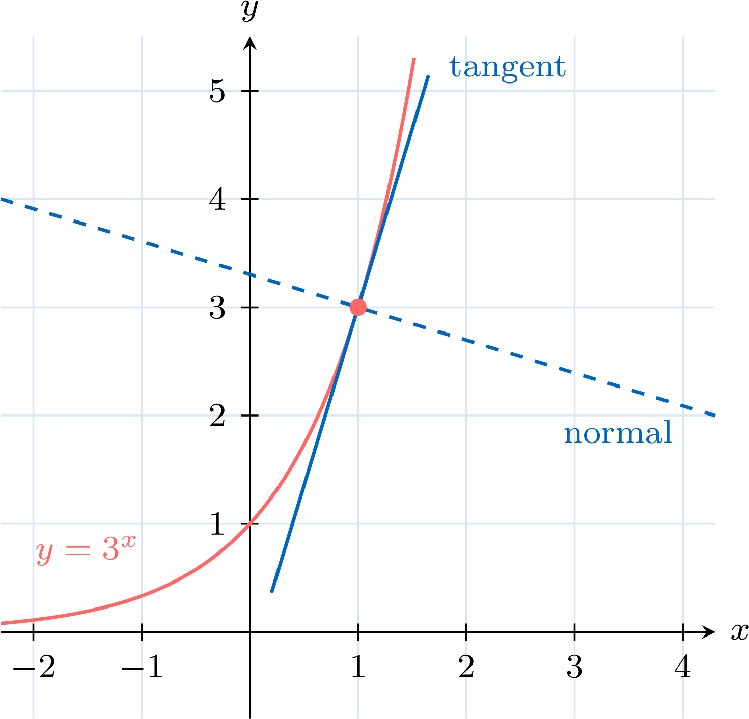
The gradient of the tangent. The derivative command, with \(3^X\) and \(X = 1\), displays about \(3.29584\) (the last digits depend on the model), kept in a memory. It is not zero, so the normal is not vertical, and its gradient is $$-\frac{1}{f'(1)} \approx -0.30341.$$ The equation of the normal. $$\begin{aligned}[t] y &= -\frac{1}{f'(1)}(x - 1) + f(1) &&\text{(equation of the normal)} \\ &\approx -0.30341(x - 1) + 3 \\ &\approx -0.30341x + 3.30341. &&\text{(expand)} \end{aligned}$$ Rounded at the end: \(y \approx -0.303x + 3.30\). Some calculators draw the normal directly (normal tool of the sketch menu) and display its equation: a check. On the screen, as on the figure, the normal looks perpendicular to the tangent only when both axes have the same unit.
Skills to practice
- Finding the Equation of a Normal
II
Increasing and Decreasing Functions
II.1
The Sign of the Derivative
When we draw the graph of a function, we may notice that the function is increasing or decreasing over particular intervals.
Definition — Increasing and Decreasing Functions
Let \(I\) be an interval contained in the domain of a function \(f\). - \(f\) is increasing on \(I\) if for all \(x_1, x_2 \in I\) such that \(x_1 < x_2\), we have \(f(x_1) \leq f(x_2)\); it is strictly increasing if \(f(x_1) < f(x_2)\).
- \(f\) is decreasing on \(I\) if for all \(x_1, x_2 \in I\) such that \(x_1 < x_2\), we have \(f(x_1) \geq f(x_2)\); it is strictly decreasing if \(f(x_1) > f(x_2)\).
Example
The function \(f(x) = x^2\) is decreasing on the interval \((-\infty, 0)\) and increasing on the interval \((0, \infty)\). 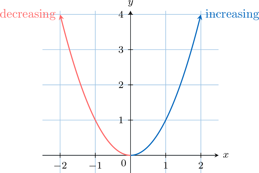
The derivative of a function, \(f'\), gives the gradient of the tangent at any point on the curve \(y=f(x)\). This allows us to determine the intervals where the function is increasing or decreasing.
A function is increasing where the gradient of its tangent is positive, and decreasing where the gradient of its tangent is negative. 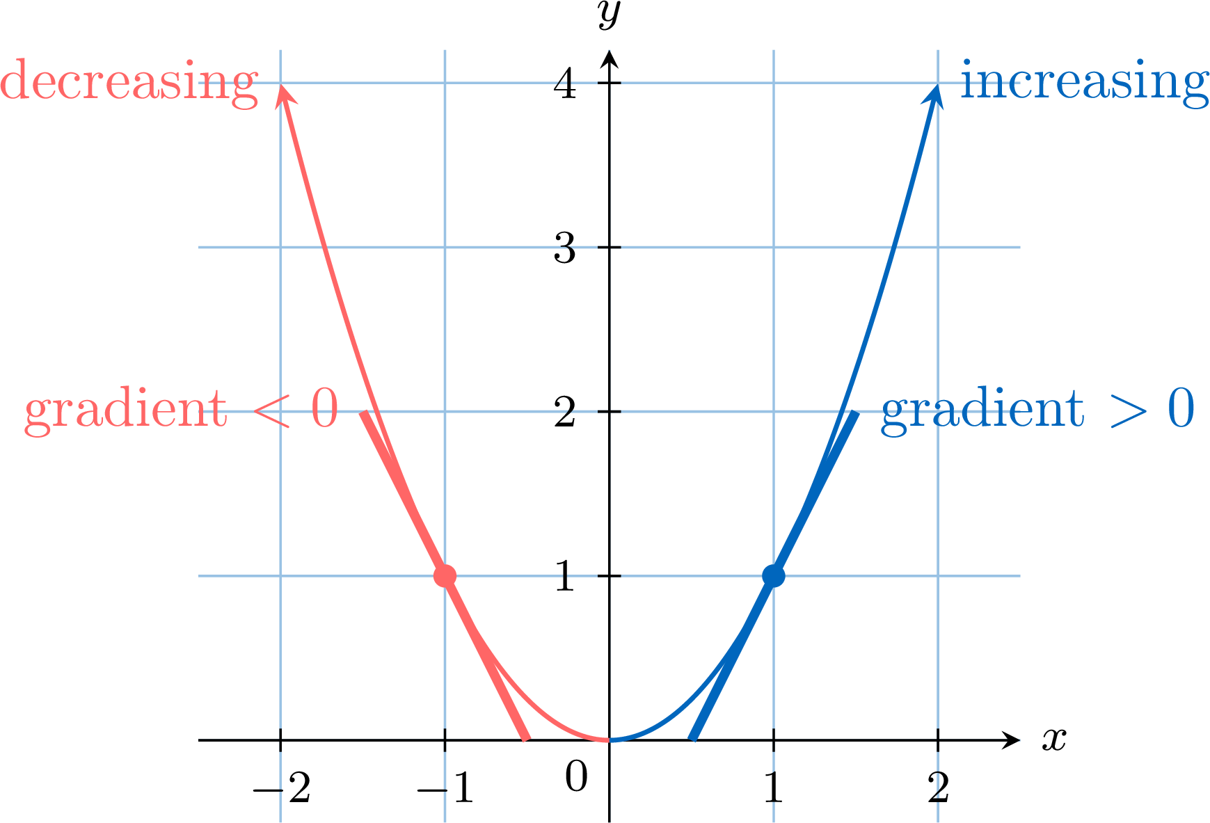
A function is increasing where the gradient of its tangent is positive, and decreasing where the gradient of its tangent is negative.
Proposition — Strict Sign of the Derivative and Monotonicity
For a function \(f\) that is differentiable on an interval \(I\): - If \(f'(x) > 0\) for all \(x \in I\), then \(f\) is strictly increasing on \(I\).
- If \(f'(x) < 0\) for all \(x \in I\), then \(f\) is strictly decreasing on \(I\).
Proposition — From the Variations to the Sign of the Derivative
Let \(f\) be a function differentiable on an interval \(I\). - If \(f\) is increasing on \(I\), then \(f'(x) \geq 0\) for all \(x \in I\).
- If \(f\) is decreasing on \(I\), then \(f'(x) \leq 0\) for all \(x \in I\).
- If \(f\) is constant on \(I\), then \(f'(x) = 0\) for all \(x \in I\).
Let \(a \in I\) and suppose that \(f\) is increasing on \(I\). For \(x \in I\) with \(x \neq a\), consider the rate of change \(\dfrac{f(x)-f(a)}{x-a}\).
If \(f\) is decreasing, the same reasoning gives a quotient less than or equal to \(0\), hence \(f'(a) \leq 0\). If \(f\) is constant, \(f(x) - f(a) = 0\): the rate of change is \(0\) and so is \(f'(a)\).
- If \(x < a\): since \(f\) is increasing, \(f(x) \leq f(a)\), so \(f(x) - f(a) \leq 0\) and \(x - a < 0\). The quotient of two numbers of the same sign is positive or zero.
- If \(x > a\): \(f(x) \geq f(a)\), so \(f(x) - f(a) \geq 0\) and \(x - a > 0\). Again the quotient is positive or zero.
If \(f\) is decreasing, the same reasoning gives a quotient less than or equal to \(0\), hence \(f'(a) \leq 0\). If \(f\) is constant, \(f(x) - f(a) = 0\): the rate of change is \(0\) and so is \(f'(a)\).
Proposition — Sign of the Derivative and Direction of Variation
The derivative may vanish at isolated points without changing the variations: if \(f'(x) \geq 0\) on \(I\), then \(f\) is increasing on \(I\), and if moreover \(f'\) vanishes only at a finite number of points, \(f\) is even strictly increasing. For instance \(f(x) = x^3\) has \(f'(x) = 3x^2 \geq 0\), which is zero only at \(x = 0\), and \(x^3\) is increasing on \(\mathbb{R}\). Together with the proposition “From the Variations to the Sign of the Derivative”: on an interval, \(f\) is increasing if and only if \(f' \geq 0\), and decreasing if and only if \(f' \leq 0\). Method — Sign Diagram and Table of Variations
A sign diagram for the derivative, \(f'\), shows where the function is increasing or decreasing. This information is organised in a table of variations. Example
Find the variations of the function \(f(x)=x^2\).
The derivative of the function \(f(x)=x^2\) is \(f'(x)=2x\). 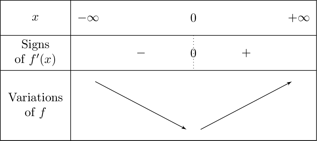
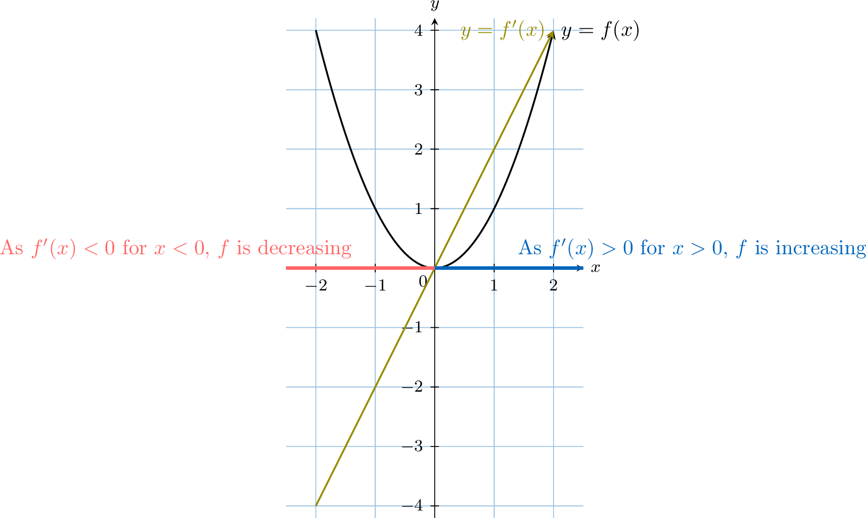
- The derivative \(f'(x)\) is negative on \((-\infty, 0)\), so the function \(f(x)\) is decreasing on \((-\infty, 0]\).
- The derivative \(f'(x)\) is positive on \((0,+\infty)\), so the function \(f(x)\) is increasing on \([0,+\infty)\).
Skills to practice
- Reading the Sign of the Derivative
- Determining Variations from a Graph
- Studying the Variations of a Function
III
Stationary Points and Extrema
III.1
Local and Global Extrema
Definition — Global Extrema
Let \(f\) be a function with domain \(D\). - \(f\) has a global maximum at \(x=c\) if \(f(c) \ge f(x)\) for all \(x\) in \(D\). The value \(f(c)\) is the maximum value of \(f\).
- \(f\) has a global minimum at \(x=c\) if \(f(c) \le f(x)\) for all \(x\) in \(D\). The value \(f(c)\) is the minimum value of \(f\).
Example
For \(f(x)=(x-1)^2-1\), the point \((1,-1)\) is a global minimum, since \(f(x) \ge f(1)\) for all \(x \in \mathbb{R}\). 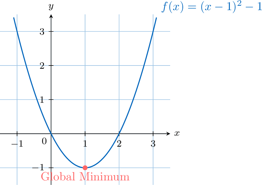
Definition — Local Extrema
Let \(f\) be a function. - \(f\) has a local maximum at \(x=c\) if there is an open interval \(I\) containing \(c\) such that \(f(c) \ge f(x)\) for all \(x\) in \(I\).
- \(f\) has a local minimum at \(x=c\) if there is an open interval \(I\) containing \(c\) such that \(f(c) \le f(x)\) for all \(x\) in \(I\).
Example
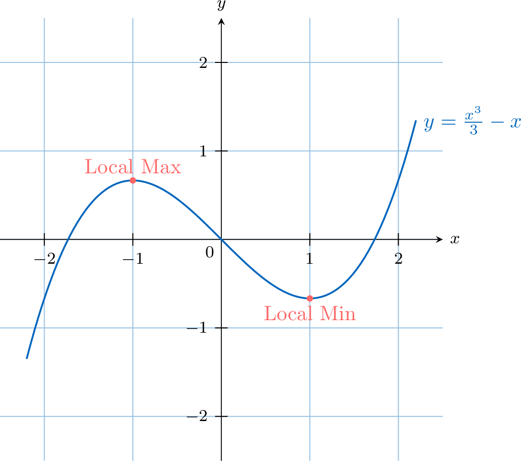
The function \(f(x) = \frac{x^3}{3} - x\) has a local maximum at \(x=-1\) and a local minimum at \(x=1\). 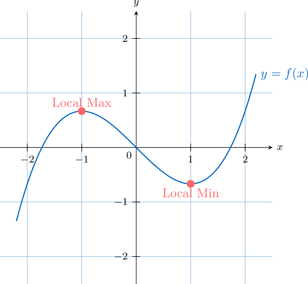
Definition — Stationary Point
A stationary point of a function \(f\) is a point \((c, f(c))\) on the curve where the tangent is horizontal, which means \(f^{\prime}(c)=0\). Proposition — Local Extrema and Stationary Points
Let \(f\) be a function defined on an open interval \(I\), and let \(c\in I\).If \(f\) has a local maximum or a local minimum at \(x=c\) and if \(f\) is differentiable at \(c\), then$$ f'(c)=0. $$
The condition \(f'(x_0) = 0\) is necessary for a local extremum at an interior point where \(f\) is differentiable, but it is not sufficient: for \(f(x) = x^3\), \(f'(0) = 0\) and yet \(f\) has no extremum at \(0\), since it keeps increasing. A function can also have an extremum at a point where it is not differentiable (\(|x|\) at \(0\)) or at an endpoint of its interval (\(x^2\) on \([1, 3]\) has its minimum at \(1\) and its maximum at \(3\)): the proposition only concerns interior points where \(f\) is differentiable.
Proposition — First Derivative Test for Local Extrema
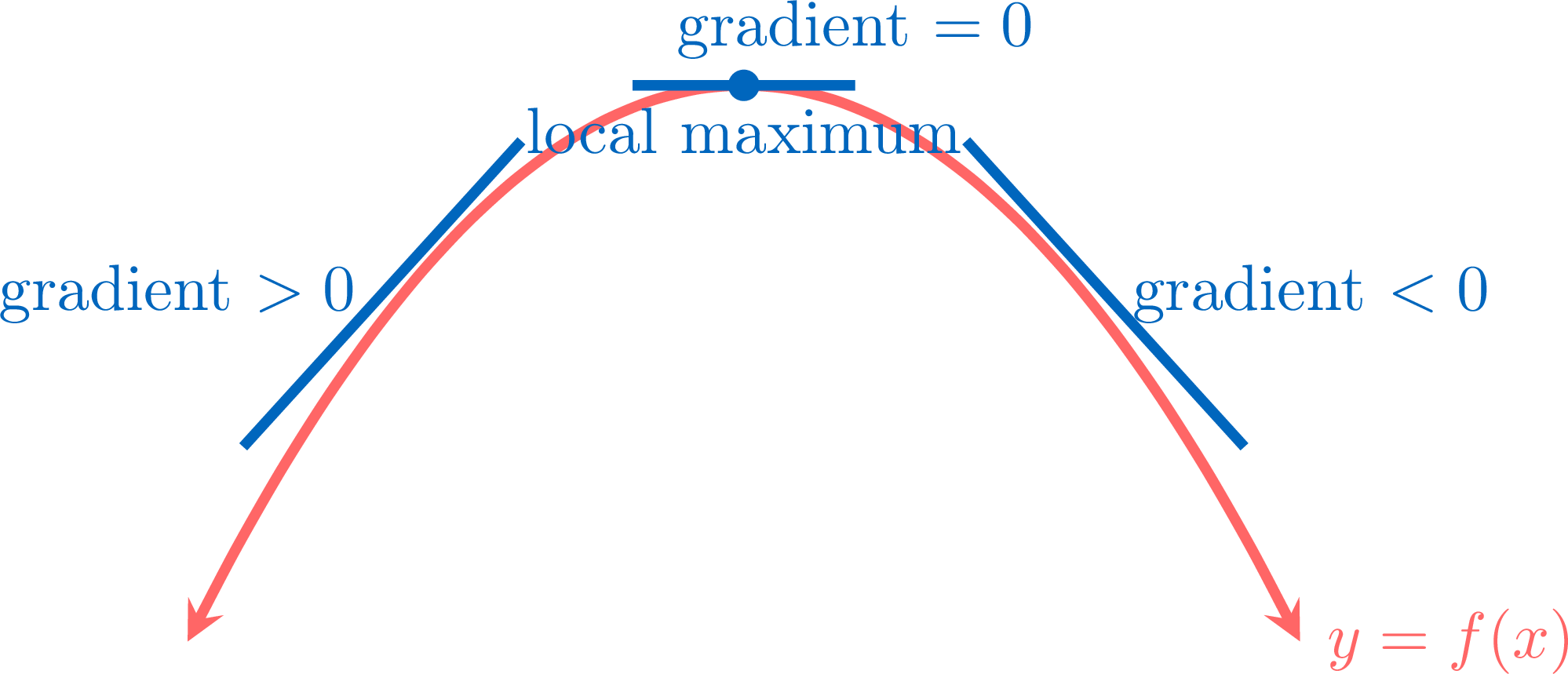
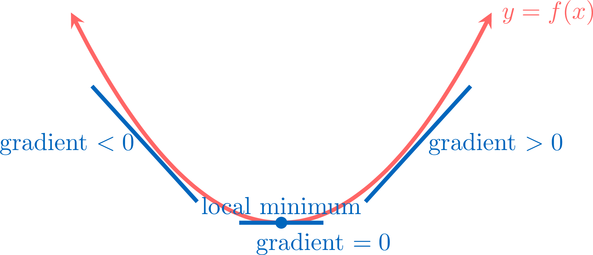
Let \(c\) be a number such that \(f'(c) = 0\). - If \(f^{\prime}(x)\) changes sign from positive to negative at \(x=c\), then \(f\) has a local maximum at \(c\).
- If \(f^{\prime}(x)\) changes sign from negative to positive at \(x=c\), then \(f\) has a local minimum at \(c\).
Example
Find and classify the stationary points of \(f(x) = \frac{1}{3}x^3 - x\). - Find the derivative:$$ f'(x) = x^2 - 1. $$
- Find stationary points by solving \(f'(x)=0\):$$ \begin{aligned} x^2 - 1 &= 0 \\ (x-1)(x+1) &= 0.\end{aligned}$$ The stationary points are at \(x=-1\) and \(x=1\).
- Create the sign diagram for \(f'(x)\):
The derivative \(f'(x)=x^2-1\) is an upward-opening parabola with roots at \(-1\) and \(1\). It is positive outside the roots and negative between them. - Draw the table of variations and classify points:
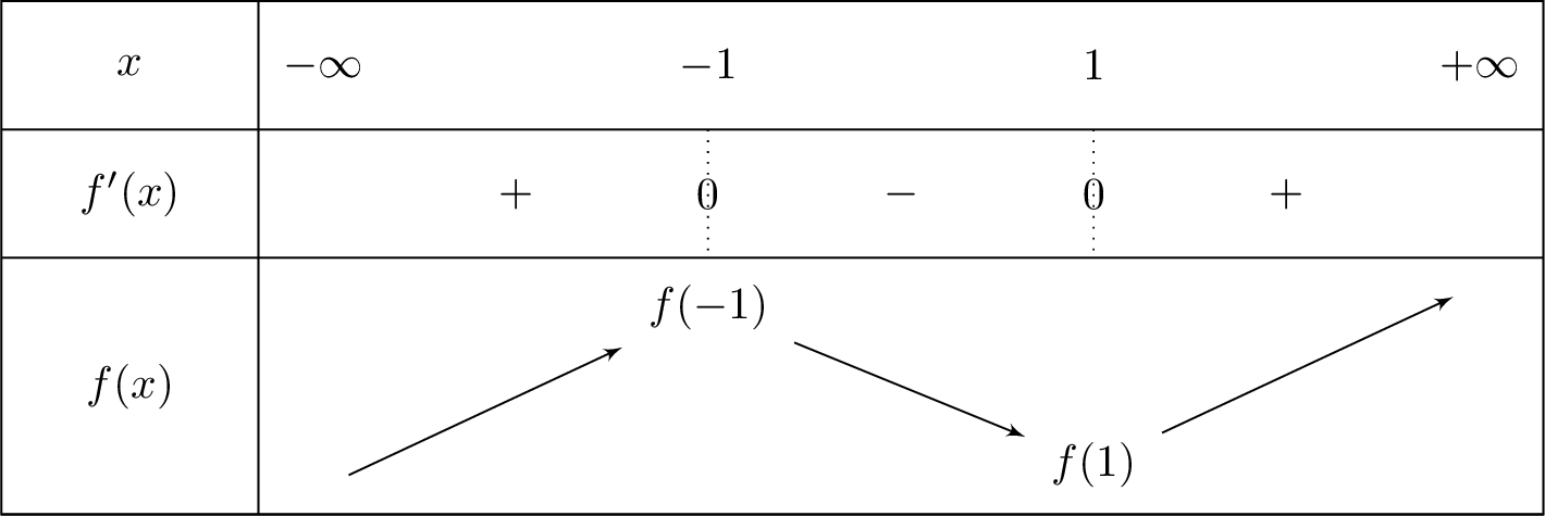
- At \(x=-1\), the sign of \(f'(x)\) changes from \(+\) to \(-\). Thus, there is a local maximum at \(x=-1\).$$f(-1) = \frac{1}{3}(-1)^3 - (-1) = \frac{2}{3}.$$
- At \(x=1\), the sign of \(f'(x)\) changes from \(-\) to \(+\). Thus, there is a local minimum at \(x=1\).$$f(1) = \frac{1}{3}(1)^3 - 1 = -\frac{2}{3}.$$
Proposition — The Quadratic Function Revisited
Let \(f(x) = ax^2 + bx + c\) with \(a \neq 0\). Then \(f\) is differentiable on \(\mathbb{R}\), \(f'(x) = 2ax + b\), and \(f'\) vanishes at \(x_0 = -\dfrac{b}{2a}\) while changing sign. - If \(a > 0\): \(f\) is decreasing on \((-\infty, x_0]\) and increasing on \([x_0, \infty)\); it has a minimum, equal to \(f(x_0)\), at \(x_0\).
- If \(a < 0\): \(f\) is increasing on \((-\infty, x_0]\) and decreasing on \([x_0, \infty)\); it has a maximum, equal to \(f(x_0)\), at \(x_0\).
\(f'(x) = 2ax + b\) is a linear function with gradient \(2a\); it vanishes at \(x_0 = -\dfrac{b}{2a}\). If \(a > 0\), then \(2a > 0\), so \(f'(x) < 0\) for \(x < x_0\) and \(f'(x) > 0\) for \(x > x_0\): \(f\) is decreasing then increasing, and \(f'\) vanishes at \(x_0\) while changing sign from \(-\) to \(+\), so \(f\) has a minimum at \(x_0\). If \(a < 0\), all the signs are reversed: \(f\) is increasing then decreasing, with a maximum at \(x_0\).
Example
Let \(f(x) = -2x^2 + 8x - 3\). Compute \(f'(x)\), build the table of variations of \(f\) and give its extremum.
\(f'(x) = -4x + 8 = -4(x - 2)\), which vanishes at \(x_0 = 2\). Since \(-4 < 0\), \(f'(x) > 0\) for \(x < 2\) and \(f'(x) < 0\) for \(x > 2\). With \(f(2) = -8 + 16 - 3 = 5\): 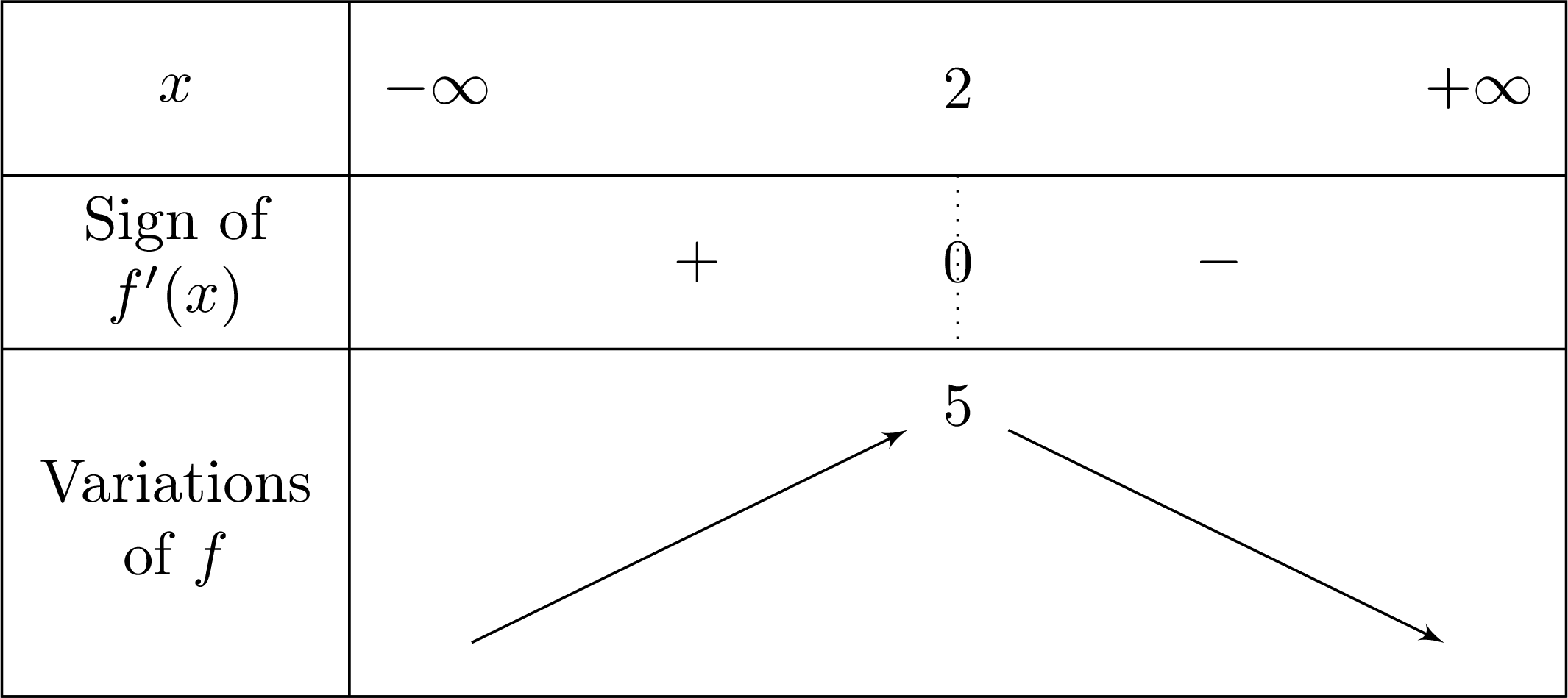
\(f\) has a maximum, equal to \(5\), at \(x = 2\): this is the vertex \((2, 5)\) of the parabola, which opens downwards since \(a = -2 < 0\).
Skills to practice
- Identifying Extrema
- Finding and Classifying Stationary Points
III.2
Stationary Points with Technology
Method — Locating Stationary Points with the Graph of the Derivative
When the equation \(f'(x) = 0\) cannot be solved by hand, a graphing calculator locates the stationary points of \(f\) from the graph of \(f'\), which it generates from the expression of \(f\) alone: - Enter \(f(x)\) as \(Y_1\), then generate \(f'\) as \(Y_2\): the derivative command applied to \(Y_1\) at the point \(X\), written \(\frac{\mathrm{d}}{\mathrm{d}X}(Y_1)\big|_{X=X}\) on most models. When the expression of \(f'(x)\) is known, enter it instead.
- Solve \(f'(x) = 0\): the zero tool applied to \(Y_2\), with bounds on either side of each \(x\)-intercept, gives the \(x\)-coordinates of the stationary points of \(f\). Store each value. The zero tool looks for a change of sign, so it may miss a point where the graph of \(f'\) touches the axis without crossing it: such a point is a local maximum or minimum of \(f'\) of value \(0\), found with the maximum or minimum tool applied to \(Y_2\).
- Classify each stationary point with the sign of \(f'\) on either side, read on the graph of \(Y_2\): where it crosses the \(x\)-axis from above to below, \(f\) has a local maximum; from below to above, a local minimum; where it touches the axis without crossing, neither. These readings concern the isolated zeros of \(f'\), where the graph of \(Y_2\) meets the axis at a single point; where the graph of \(Y_2\) runs along the \(x\)-axis over a whole interval, \(f' = 0\) there and \(f\) is constant on that interval.
- Compute the \(y\)-coordinates with the value tool on \(Y_1\), at the stored \(x\)-coordinates, and report the coordinates to 3 significant figures.
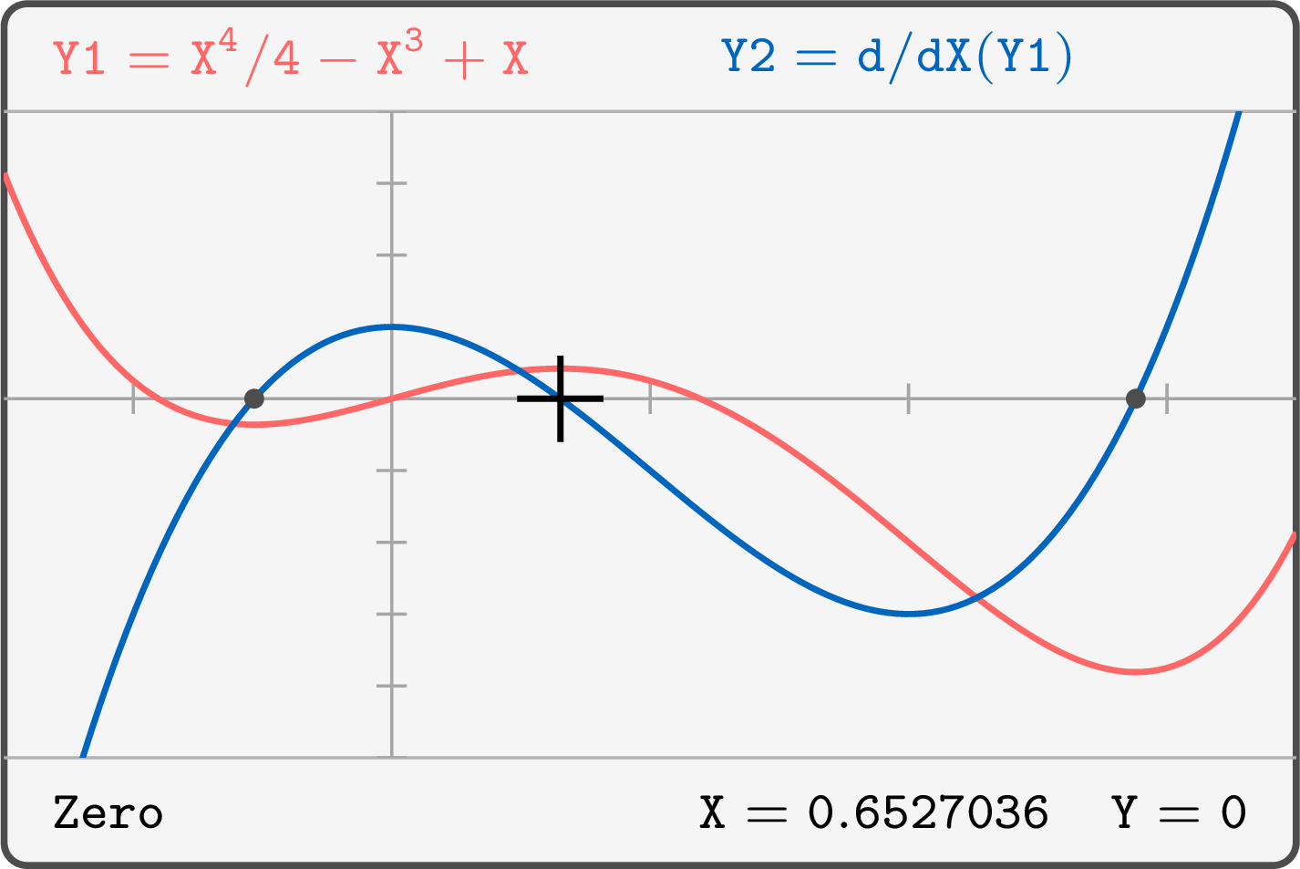
The mock-up generates the graph of \(f'\) for \(f(x) = \dfrac{x^4}{4} - x^3 + x\), and the zero tool finds one of its three \(x\)-intercepts: the stationary points of \(f\) are at \(x \approx -0.532\), \(x \approx 0.653\) and \(x \approx 2.88\).
Example
Let \(f(x) = x^4 - 3x^3 + x + 2\), for \(-1 \le x \le 3\). - Use technology to generate the graph of \(f'\), and find the \(x\)-coordinates of the stationary points of \(f\), to 3 significant figures.
- Determine the nature of each stationary point, and its coordinates.
- Find the greatest value and the least value of \(f\) on \([-1, 3]\).
- \(f\) is a polynomial function, differentiable on \([-1, 3]\), and \(f'(x) = 4x^3 - 9x^2 + 1\): this equation of degree \(3\) has no integer or simple fractional root, so the calculator solves it. With \(Y_1 = X^4 - 3X^3 + X + 2\) and \(Y_2 = \frac{\mathrm{d}}{\mathrm{d}X}(Y_1)\big|_{X=X}\), in the window \(-1 \le x \le 3\), \(-6 \le y \le 6\), the graph of \(f'\) crosses the \(x\)-axis three times. The zero tool displays \(X = -0.3123563\), \(X = 0.3640907\) and \(X = 2.1982656\): the stationary points are at \(x \approx -0.312\), \(x \approx 0.364\) and \(x \approx 2.20\). The polynomial solver, applied to \(4x^3 - 9x^2 + 1 = 0\), returns the same three values.
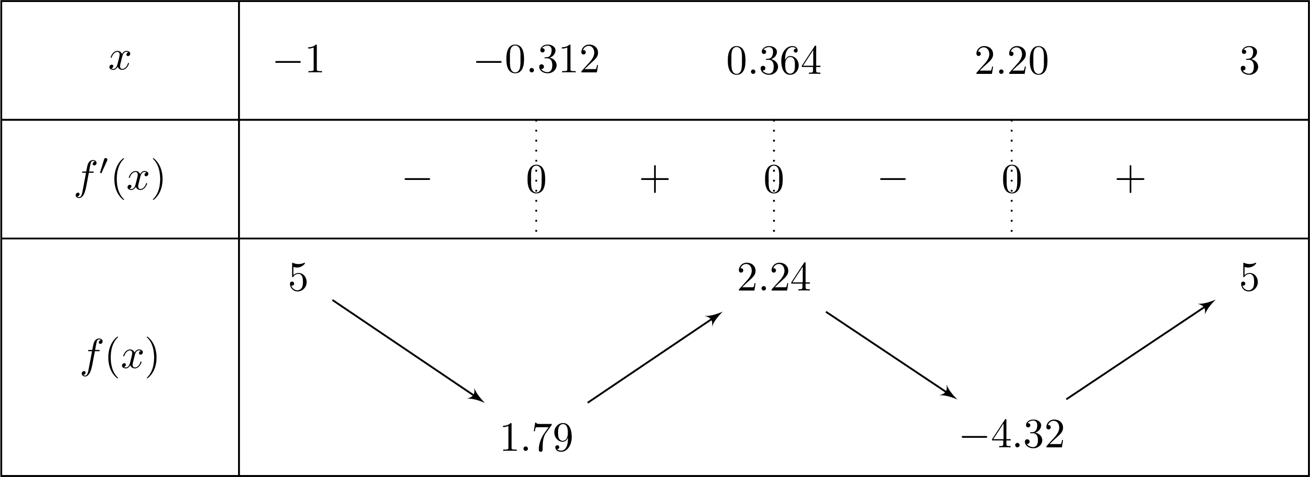
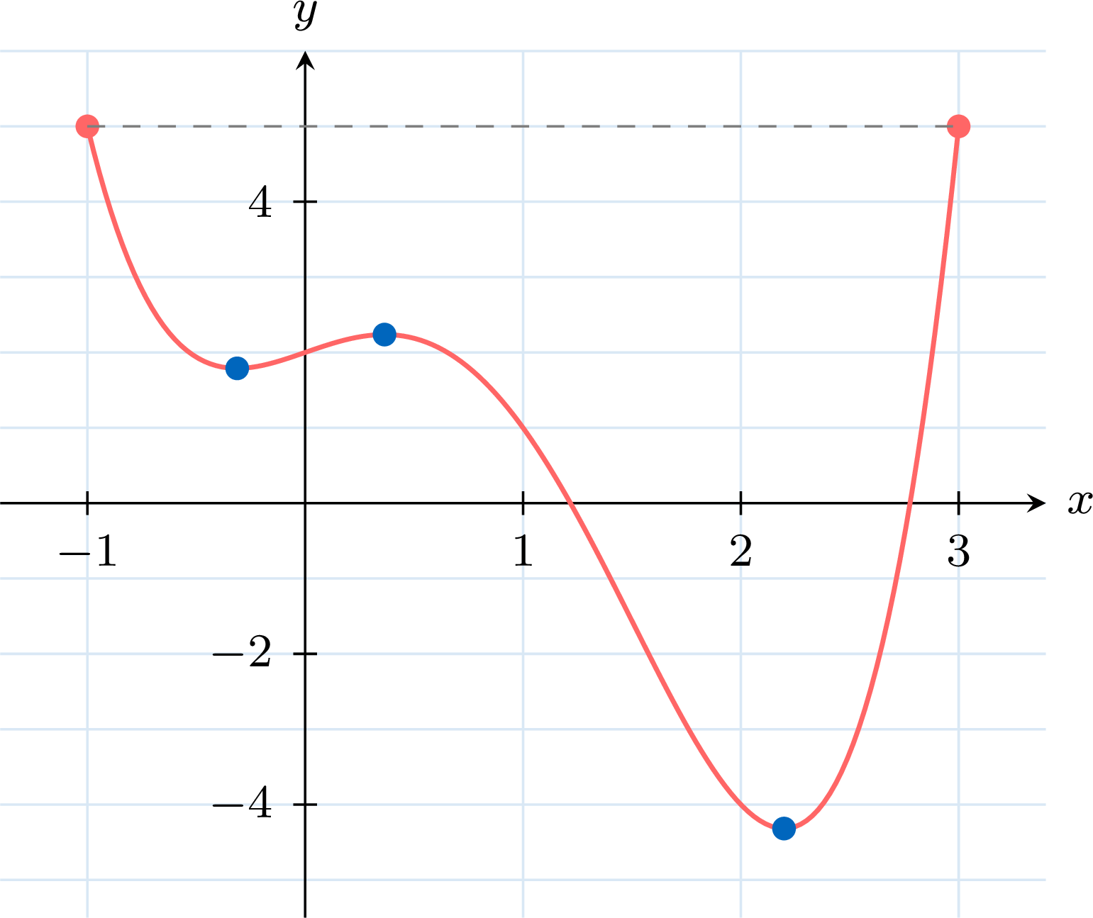
- On the screen, the graph of \(f'\) is below the \(x\)-axis before \(-0.312\), above it between \(-0.312\) and \(0.364\), below it between \(0.364\) and \(2.20\), and above it after \(2.20\). By the first derivative test, \(f\) has a local minimum at \(x \approx -0.312\), a local maximum at \(x \approx 0.364\) and a local minimum at \(x \approx 2.20\). The value tool on \(Y_1\), at the stored \(x\)-coordinates, displays \(1.7885894\), \(2.2368696\) and \(-4.3184277\): the points are \((-0.312, 1.79)\), \((0.364, 2.24)\) and \((2.20, -4.32)\).
- At the endpoints, \(f(-1) = 1 + 3 - 1 + 2 = 5\) and \(f(3) = 81 - 81 + 3 + 2 = 5\). The table of variations gathers the values:
Skills to practice
- Locating Stationary Points with Technology
IV
Going further
Skills to practice
- Diagnosing and Correcting Errors
- Solving Exam-Style Problems on Curves
- Quiz
Jump to section