International Baccalaureate · DP 2: Analysis and Approaches SL
Applications of Differentiation
I
Optimisation
I.1
Optimising a Quadratic Function
Recappreviously studied — click to reread
Method — Optimising a Quadratic Function
- Read the problem to identify the quantity to be maximised or minimised.
- Define variables and write a quadratic function that models this quantity.
- Find the coordinates of the vertex \((h,k)\) of the parabola.
- \(h = -\frac{b}{2a}\) gives the input value (e.g., time, length, price) where the optimum occurs.
- \(k = f(h)\) gives the optimal (maximum or minimum) value itself.
- Check that \(h\) is an allowed value of the variable (for instance, a length or a time is positive).
- Answer the question in the context of the problem, making sure to include units.
Skills to practice
- Optimising a Quadratic Function
I.2
Optimisation Problems
Optimisation is one of the most important applications of differential calculus. It involves finding the maximum or minimum value that a function can take, subject to given conditions. In many problems, this corresponds to finding the global maximum or minimum of that function on a specified domain.
Definition — Optimisation
Optimisation is the process of finding a maximum or minimum value of a function, known as the objective function, subject to a set of constraints (or over a specified domain). The solution that achieves this is called the optimal solution. Example
In machine learning, a key goal is to minimise a loss (error) function by adjusting model parameters. This optimisation process underlies how modern neural networks are trained. Method — Solving Optimisation Problems
- Model: Identify the quantity to be optimised and express it as a function of a single variable (for example \(f(x)\)). Use any given constraints to eliminate other variables. Determine the feasible domain for \(x\).
- Differentiate: Check that \(f\) is differentiable on the domain, then find the first derivative of the function, \(f'(x)\).
- Find Stationary Points: Solve \(f'(x)=0\) for \(x\) in the domain.
- Test and Justify: Use the sign of the derivative (sign table of \(f'\), table of variations) to decide whether each stationary point is a local maximum, a local minimum, or neither.
- Check Endpoints: If the domain is a closed interval \([a, b]\), evaluate the function at the stationary points and also at the endpoints, \(f(a)\) and \(f(b)\), to find the global extremum on that interval.
- Conclusion: State the final answer clearly in the context of the problem, including units.
Example
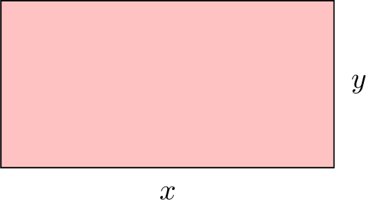
A rectangle has a perimeter of 12 cm. Find its dimensions to maximise the area. - Model: Let the length be \(x\) and the width be \(y\).
- Derivative: $$A'(x) = 6-2x.$$
- Stationary point: $$ A'(x) = 0 \implies 6-2x=0 \implies 2x=6 \implies x=3. $$
- Justification: sign of \(A'\). \(A'(x) = 6 - 2x\) is positive for \(x < 3\) and negative for \(x > 3\), so \(A\) is increasing on \([0, 3]\) and decreasing on \([3, 6]\): \(x = 3\) gives the maximum of \(A\).
- Check endpoints: The domain is the closed interval \([0,6]\). We check the area at the stationary point and at the endpoints, where \(x = 0\) and \(x = 6\) give flattened rectangles of area \(0\):
- \(A(0) = 6(0)-0^2 = 0\)
- \(A(3) = 6(3)-3^2 = 18-9 = 9\)
- \(A(6) = 6(6)-6^2 = 0\)
- Conclusion: The area is maximised when the length is \(x=3\) cm. The corresponding width is \(y=6-3=3\) cm. The rectangle with maximum area is therefore a square of side 3 cm, with an area of \(9\text{ cm}^2\).
Example
A closed storage container with a square base must contain a volume of \(8\) m\(^3\). Find the dimensions that minimise the total surface area of the container. - Model: Let \(x\) be the side of the square base and \(h\) the height. The volume constraint gives $$x^2 h = 8 \implies h = \frac{8}{x^2}.$$ The surface consists of the base, the top and four lateral faces: $$S = 2x^2 + 4xh = 2x^2 + 4x \cdot \frac{8}{x^2} = 2x^2 + \frac{32}{x}.$$ The domain is \(x \in (0, \infty)\) — an open interval: there are no endpoints to check, so the justification must come from the variations.
- Derivative: $$S'(x) = 4x - \frac{32}{x^2} = \frac{4x^3 - 32}{x^2}.$$
- Stationary point: \(S'(x) = 0 \iff 4x^3 = 32 \iff x^3 = 8 \iff x = 2\).
- Test and justify: the sign of \(S'(x)\) is the sign of \(4x^3 - 32\): negative for \(0 < x < 2\), positive for \(x > 2\). So \(S\) decreases on \((0, 2]\) and increases on \([2, \infty)\): the variation table shows that \(x = 2\) gives the global minimum on the whole domain — no endpoint check is possible, and none is needed.
- Conclusion: \(x = 2\) m and \(h = \frac{8}{4} = 2\) m: the optimal container is a cube of side \(2\) m, with total surface \(S(2) = 2(4) + \frac{32}{2} = 24\) m\(^2\).
Skills to practice
- Setting Up an Optimisation Problem
- Solving Optimisation Problems
- Solving Optimisation Problems in Context
I.3
An Optimum at an End Point
Example
A wire \(20\) cm long is cut into two pieces. A piece of length \(x\) cm is bent into a square, and the other piece into a circle. The values \(x = 0\) and \(x = 20\) mean that the whole wire makes a single shape, so \(0 \le x \le 20\). - Show that the total area enclosed is \(A(x) = \dfrac{x^2}{16} + \dfrac{(20 - x)^2}{4\pi}\) cm\(^2\).
- Find the value of \(x\) for which \(A'(x) = 0\), and show that it gives the least total area.
- Where should the wire be cut to enclose the greatest total area?
- The square has perimeter \(x\), so its side is \(\dfrac{x}{4}\) and its area \(\dfrac{x^2}{16}\). The circle has circumference \(2\pi\rho = 20 - x\), so its radius is \(\rho = \dfrac{20 - x}{2\pi}\) and its area is $$\begin{aligned}[t] \pi\rho^2 &= \pi \times \frac{(20 - x)^2}{4\pi^2} && \text{(area of a disc, } \rho = \tfrac{20 - x}{2\pi}\text{)} \\ &= \frac{(20 - x)^2}{4\pi}. \end{aligned}$$ Adding the two areas gives \(A(x) = \dfrac{x^2}{16} + \dfrac{(20 - x)^2}{4\pi}\).
- Since \((20 - x)^2 = 400 - 40x + x^2\) has derivative \(-40 + 2x = -2(20 - x)\), $$\begin{aligned}[t] A'(x) &= \frac{2x}{16} - \frac{2(20 - x)}{4\pi} && \text{(power rule, term by term)} \\
&= \frac{x}{8} - \frac{20 - x}{2\pi} \\
&= \frac{\pi x - 4(20 - x)}{8\pi} && \text{(common denominator } 8\pi\text{)} \\
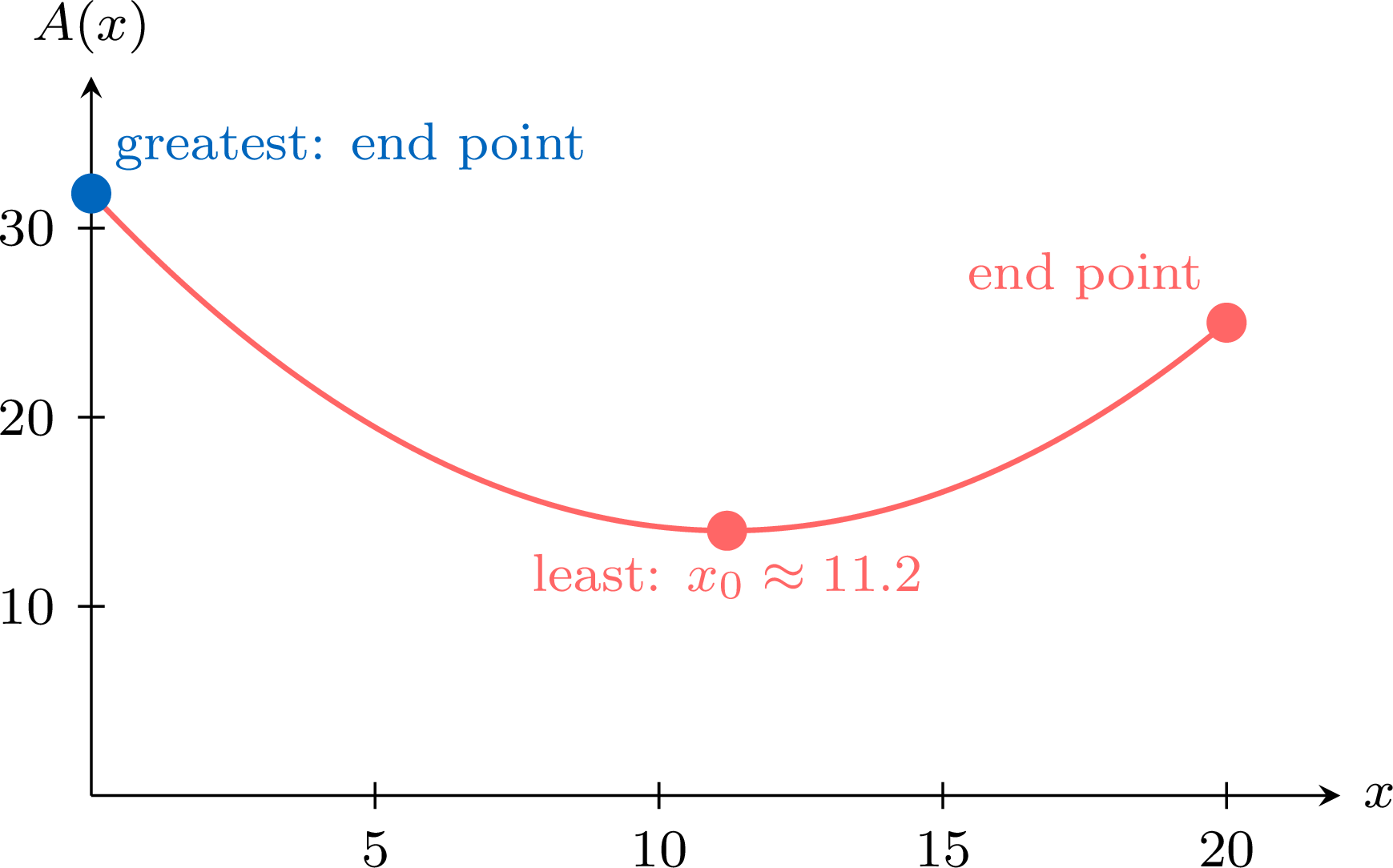
&= \frac{(\pi + 4)x - 80}{8\pi}. \end{aligned}$$ So \(A'(x) = 0\) for \(x_0 = \dfrac{80}{\pi + 4} \approx 11.2\). Since \(8\pi > 0\) and \(\pi + 4 > 0\), \(A'(x)\) has the sign of \((\pi + 4)x - 80\): negative for \(x < x_0\), positive for \(x > x_0\).
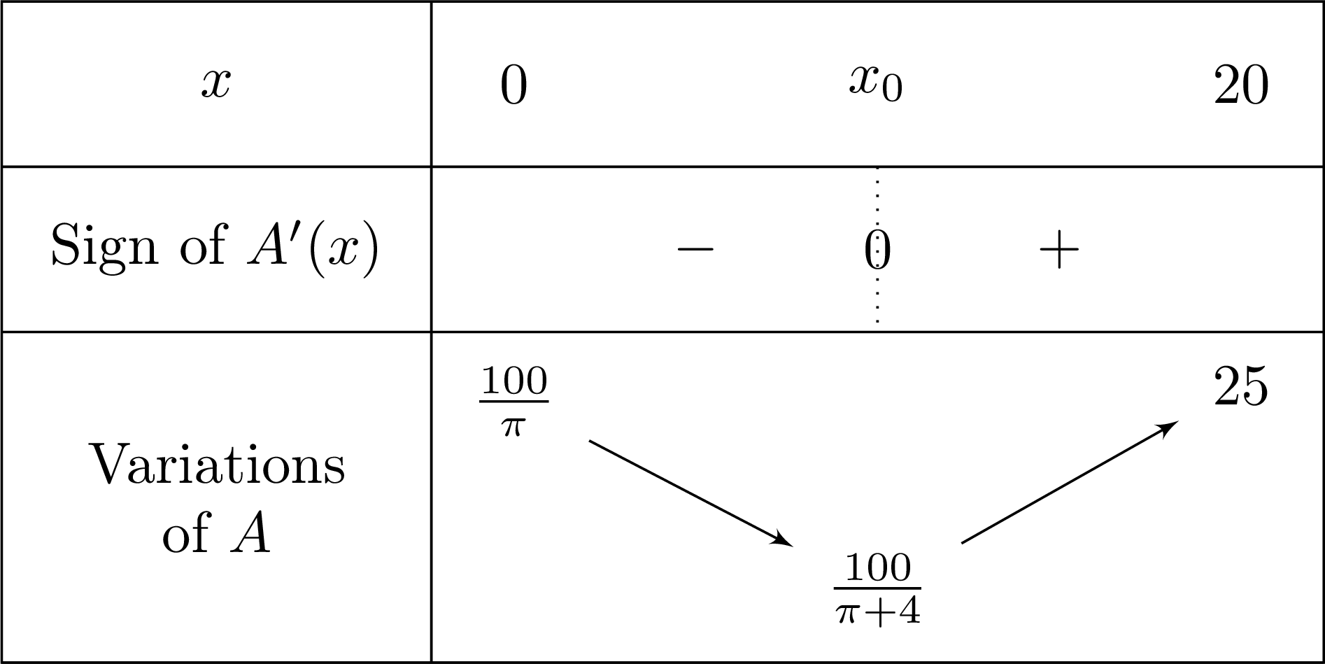
- The only stationary point is a minimum: the greatest value of \(A\) on \([0, 20]\) is at an end point. Compare the values at the end points: $$A(0) = \frac{400}{4\pi} = \frac{100}{\pi} \approx 31.8 \qquad \text{and} \qquad A(20) = \frac{400}{16} = 25.$$ Since \(\pi < 4\), \(\dfrac{100}{\pi} > \dfrac{100}{4} = 25\). The greatest total area, \(\dfrac{100}{\pi} \approx 31.8\) cm\(^2\), is reached for \(x = 0\): the wire is not cut, and all of it is bent into a circle.
Skills to practice
- Finding an Optimum at an End Point
I.4
Optimisation with Technology
Example
An oil platform \(P\) stands \(4\) km off a straight coast; \(A\) is the point of the coast nearest to \(P\), and a refinery \(R\) stands on the coast, \(10\) km from \(A\). A pipeline runs straight under the sea from \(P\) to a point \(M\) of the coast between \(A\) and \(R\), with \(AM = x\) km, then along the coast from \(M\) to \(R\). Laying the pipeline costs \(5\) million dollars per km under the sea and \(3\) million dollars per km on land. 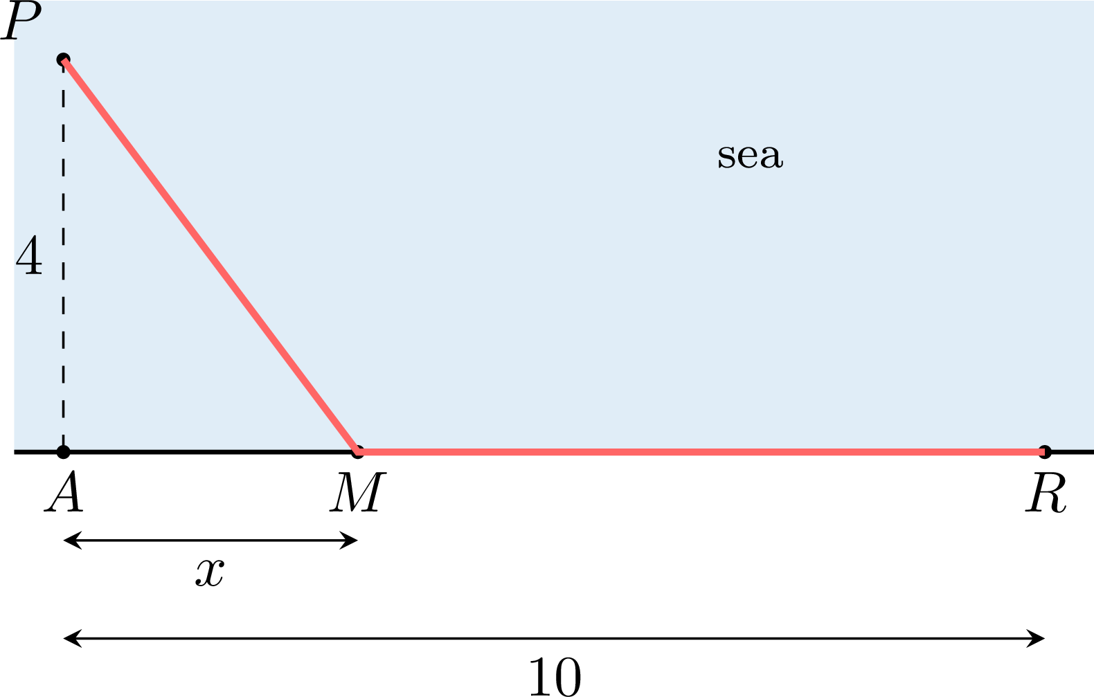
- Show that the total cost, in millions of dollars, is \(C(x) = 5\sqrt{16 + x^2} + 3(10 - x)\), for \(0 \le x \le 10\).
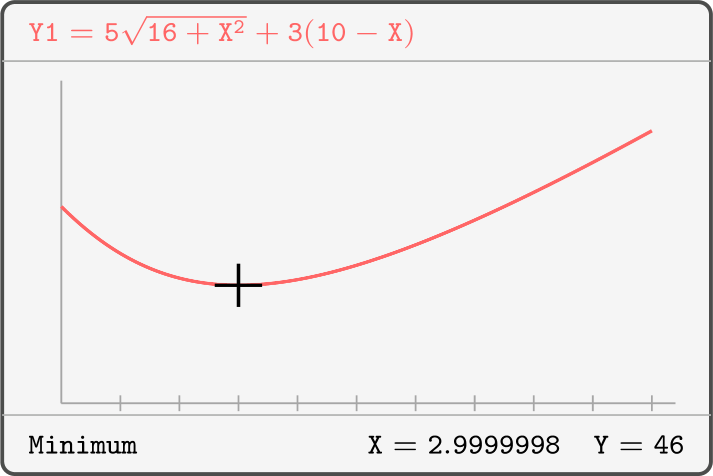
- Use technology to find where the pipeline should reach the coast, and the least cost.
- The triangle \(PAM\) is right-angled at \(A\), so by Pythagoras' theorem \(PM = \sqrt{AP^2 + AM^2} = \sqrt{16 + x^2}\) km, and \(MR = 10 - x\) km. The cost is \(5\) times the length under the sea plus \(3\) times the length on land: $$C(x) = 5\sqrt{16 + x^2} + 3(10 - x), \qquad 0 \le x \le 10.$$
- Enter \(Y_1 = 5\sqrt{16 + X^2} + 3(10 - X)\) with the window \(0 \le x \le 10\), \(40 \le y \le 56\). The curve falls, then rises: the minimum tool, with bounds on either side of the lowest point, displays \(X \approx 3\) and \(Y \approx 46\) (a value such as \(X = 2.9999998\) is the tool's approximation: the tool finds the minimum to its precision, not exactly).
Skills to practice
- Solving Optimisation Problems with Technology
II
Rates of Change
II.1
Rates of Change with Respect to Time
When a quantity \(Q\) depends on the time \(t\), the derivative \(Q'(t) = \dfrac{\mathrm{d}Q}{\mathrm{d}t}(t)\) is the instantaneous rate of change of \(Q\): how fast \(Q\) changes at the instant \(t\), the value approached by the average rate \(\dfrac{\Delta Q}{\Delta t}\) over shorter and shorter durations. Its unit is the unit of \(Q\) divided by the unit of time. Speed is the best-known example; physics and chemistry give two more.
- Power: if \(E(t)\) is the energy received by a system from the instant \(0\) to the instant \(t\), the power at the instant \(t\) is \(P(t) = \dfrac{\mathrm{d}E}{\mathrm{d}t}(t)\), in watts (\(\mathrm{W}\)) when \(E\) is in joules (\(\mathrm{J}\)) and \(t\) in seconds. When the power is constant, the energy received during a duration \(\Delta t\) is \(\Delta E = P \times \Delta t\).
- Reaction rates: during a chemical reaction, the concentration \([A](t)\) of a reactant \(A\) decreases, and its rate of disappearance is \(-\dfrac{\mathrm{d}[A]}{\mathrm{d}t}(t)\), which is non-negative; the concentration \([B](t)\) of a product \(B\) increases, and its rate of appearance is \(\dfrac{\mathrm{d}[B]}{\mathrm{d}t}(t)\). With concentrations in \(\mathrm{mol \cdot L^{-1}}\) and \(t\) in minutes, these rates are in \(\mathrm{mol \cdot L^{-1} \cdot min^{-1}}\).
Example
During a test, the energy received by a water heater from the instant \(0\) to the instant \(t\) is \(E(t) = 2t^2 + 10t\), in joules, for \(0 \leq t \leq 10\) (\(t\) in seconds). - Compute the power \(P(t)\), then \(P(0)\) and \(P(10)\).
- Compute the average power over the test, \(\dfrac{E(10) - E(0)}{10 - 0}\), and compare it with \(P(0)\) and \(P(10)\).
- $$\begin{aligned}[t] P(t) &= E'(t) &&\text{(the power is the derivative of the energy)}\\ &= 2 \times 2t + 10 &&\text{(} (t^2)' = 2t\text{, } (t)' = 1\text{)}\\ &= 4t + 10.\end{aligned}$$ The expression of \(E\) is a polynomial, differentiable at every real \(t\), including \(t = 0\) and \(t = 10\). So \(P(0) = 10~\mathrm{W}\) and \(P(10) = 50~\mathrm{W}\): the power grows during the test.
- \(E(10) = 200 + 100 = 300~\mathrm{J}\) and \(E(0) = 0\), so the average power is \(\dfrac{300}{10} = 30~\mathrm{W}\), between \(P(0) = 10~\mathrm{W}\) and \(P(10) = 50~\mathrm{W}\). A constant power of \(30~\mathrm{W}\) would give the same energy: \(30 \times 10 = 300~\mathrm{J}\).
Example
In a reaction \(A \to B\), the concentration of the reactant \(A\), in \(\mathrm{mol \cdot L^{-1}}\), is \([A](t) = \dfrac{0.5}{1 + 0.1t}\) for \(t \geq 0\) (\(t\) in minutes). Each mole of \(A\) that disappears gives one mole of \(B\), and there is no \(B\) at the start, so \([B](t) = 0.5 - [A](t)\). - Compute the rate of disappearance of \(A\) at \(t = 0\) and at \(t = 10\).
- Show that the rate of appearance of \(B\) is equal to the rate of disappearance of \(A\).
- $$\begin{aligned}[t]\frac{\mathrm{d}[A]}{\mathrm{d}t}(t) &= \frac{0 \times (1 + 0.1t) - 0.5 \times 0.1}{(1 + 0.1t)^2} &&\text{(quotient rule)}\\ &= -\frac{0.05}{(1 + 0.1t)^2}.\end{aligned}$$ The rate of disappearance is \(r(t) = \dfrac{0.05}{(1 + 0.1t)^2}\): \(r(0) = 0.05~\mathrm{mol \cdot L^{-1} \cdot min^{-1}}\) and \(r(10) = \dfrac{0.05}{2^2} = 0.0125~\mathrm{mol \cdot L^{-1} \cdot min^{-1}}\). The reaction slows down as the reactant is used up.
- \(\dfrac{\mathrm{d}[B]}{\mathrm{d}t}(t) = 0 - \dfrac{\mathrm{d}[A]}{\mathrm{d}t}(t) = r(t)\): \(B\) appears exactly as fast as \(A\) disappears.
Skills to practice
- Interpreting a Rate of Change
- Computing a Rate of Change in Context
- Modelling with Rates of Change
III
Going further
Skills to practice
- Diagnosing and Correcting Errors
- Solving Exam-Style Problems on Optimisation and Rates of Change
- Quiz
Jump to section