International Baccalaureate · DP 2: Applications and Interpretation SL

Hypothesis Testing

⌚ ~122 min ▢ 13 blocks ✓ 55 exercises ➣ Prerequisites : The Normal Distribution, Probability, Sampling and Data, Conditional Probability

I The Logic of a Test

I.1 Null and Alternative Hypotheses

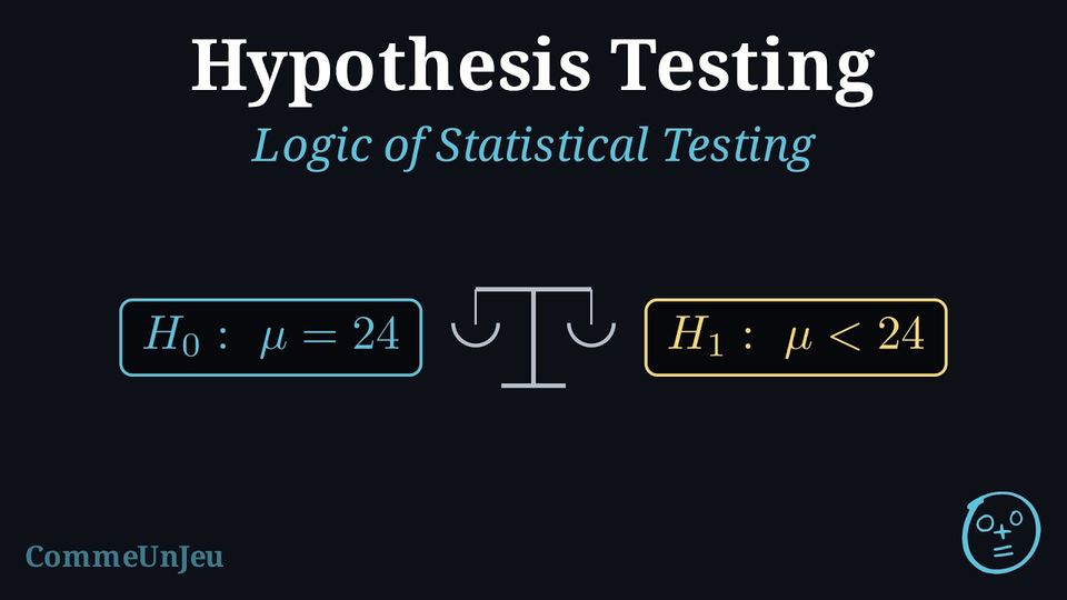
Statistical testing functions much like a court trial.

The Assumption (Innocence): We start by assuming there is no effect or no difference until proven otherwise.
The Evidence (Data): We collect data from a sample.
The Verdict: If the evidence is strong enough (beyond reasonable doubt), we reject the initial assumption.

Important: In hypothesis testing, we never “prove” $H_0$ is true. We either reject $H_0$ or fail to reject it because the evidence is not strong enough.

Report an error

Definition — Null and Alternative Hypotheses

The Null Hypothesis ($H_0$) represents the status quo, “no difference,” or “no effect.” For tests on a numerical parameter, it includes an equality ($\mu = k$, $\mu \leq k$, or $\mu \geq k$); for chi-squared tests, $H_0$ states independence or a given distribution.
The Alternative Hypothesis ($H_1$) is the claim we are trying to find evidence for. It uses strict inequalities ($\mu \neq k$, $\mu > k$, or $\mu < k$).

Example

A company claims that the average battery life of their new phone is 24 hours. A consumer group suspects the battery life is actually shorter. Write the null and alternative hypotheses.

Answer

Let $\mu$ be the true mean battery life.

$H_0: \mu = 24$ (The company's claim is true; there is no difference).
$H_1: \mu < 24$ (The consumer group's suspicion; the mean is less than claimed).

Skills to practice

Choosing the Hypotheses
Formulating Null and Alternative Hypotheses

I.2 p-value and Significance Level

Definition — p-value and $\alpha$

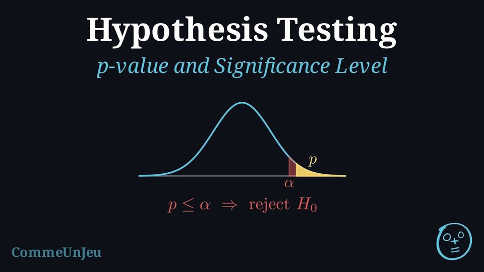
The significance level ($\alpha$) is the threshold for evidence (usually $0.05$, $0.01$, or $0.10$). It is the maximum probability, accepted in advance, of rejecting $H_0$ when it is actually true (a Type I error).
The p-value is the probability of obtaining sample results at least as extreme as the ones observed, assuming $H_0$ is true.

A small p-value means the data would be very unlikely if $H_0$ were true, so it is evidence against $H_0$.
Decision Rule:

If $p\text{-value} \leq \alpha \implies$ Reject $H_0$. (The result is statistically significant).
If $p\text{-value} > \alpha \implies$ Fail to reject $H_0$. (Not enough evidence against $H_0$).

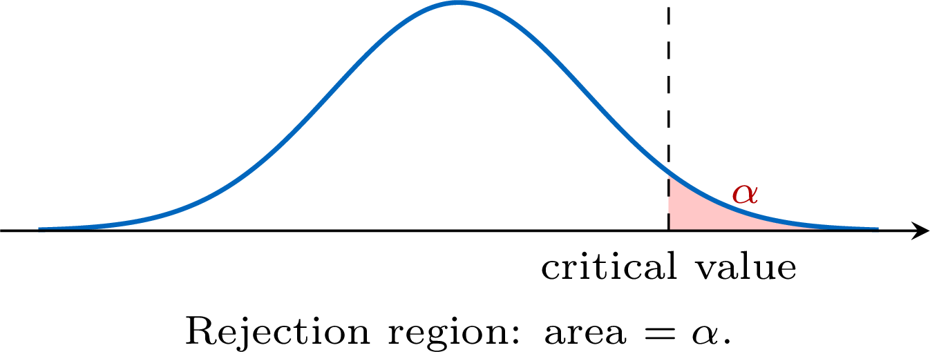
The decision rule has a clear visual meaning. If $H_0$ is true, the test statistic follows a known distribution. The p-value is the area in the tail beyond the observed statistic — the probability of a result at least as extreme. The rejection region is the set of most-extreme values whose total area is exactly $\alpha$. Rejecting $H_0$ when the statistic lands in the rejection region is the same decision as rejecting when the p-value is at most $\alpha$.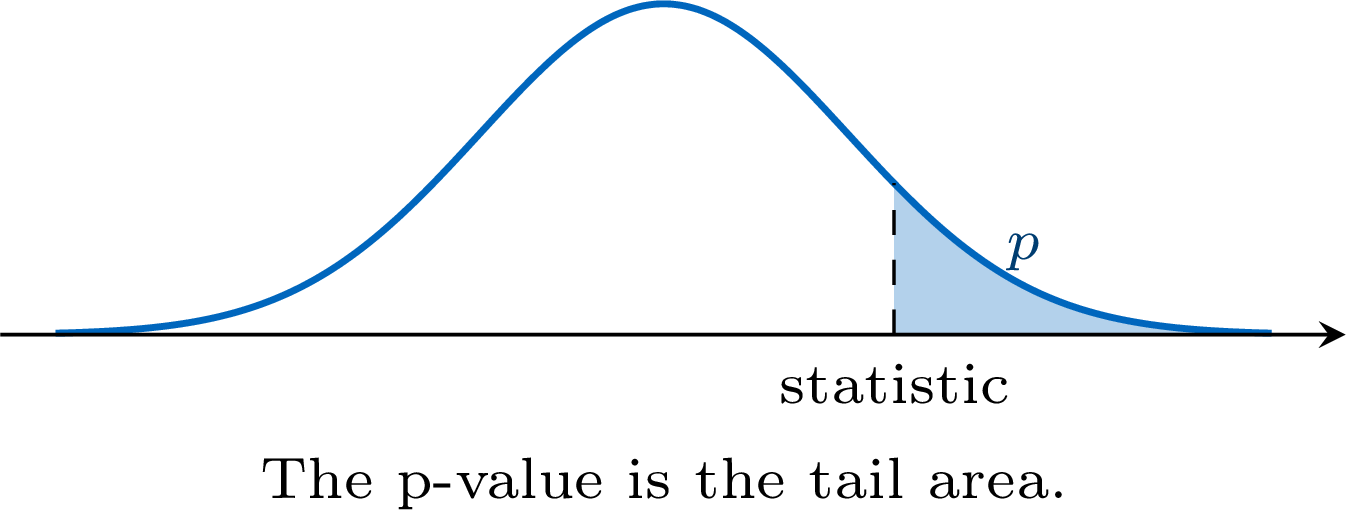

\hspace{0.4cm}

Report an error

Example

A researcher performs a hypothesis test to check if a new fertilizer increases plant growth.
The calculated $p$-value is $0.042$.
Make a conclusion for the following significance levels:

$\alpha = 0.05$ ($5\pourcent$ significance level).
$\alpha = 0.01$ ($1\pourcent$ significance level).

Answer

For $\alpha = 0.05$: $$ p\text{-value} = 0.042 < 0.05 $$ Since the $p$-value is smaller than $\alpha$, the result is statistically significant at the 5$\pourcent$ level. We reject the null hypothesis ($H_0$). There is sufficient evidence at the 5$\pourcent$ significance level to support the claim.
For $\alpha = 0.01$: $$ p\text{-value} = 0.042 \geq 0.01 $$ Since the $p$-value is greater than $\alpha$, the result is not statistically significant at this level. We fail to reject the null hypothesis ($H_0$). There is not enough evidence at the 1$\pourcent$ significance level to support the claim.

Skills to practice

Deciding from a p-value
Interpreting the p-value

I.3 The Five Steps of a Test

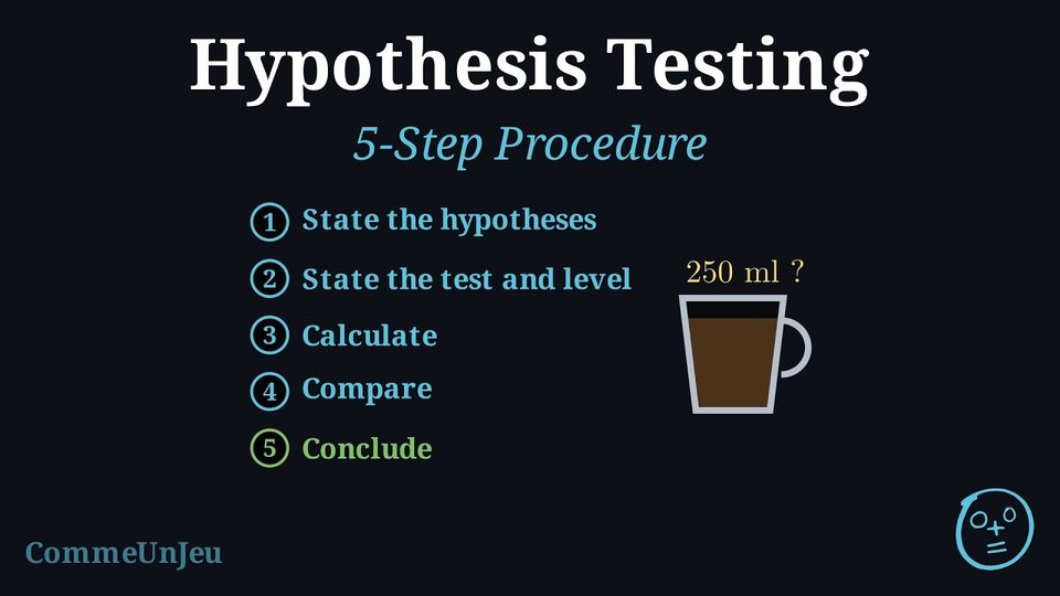
Method — Performing a Hypothesis Test

State the Hypotheses: Define the parameter (e.g., $\mu$) and write $H_0$ and $H_1$.
State the Test and Level: Identify the test (e.g., t-test) and the significance level $\alpha$.
Calculate Statistics: Use the GDC to find the test statistic and the p-value.
Compare: Explicitly compare the p-value to $\alpha$ (usually check whether $p \leq \alpha$ or $p > \alpha$).
Conclude: Write a conclusion in the context of the problem, referring to the original claim.

Example

(This example uses the one-sample t-test; the focus here is the five-step logic.)
A coffee machine is supposed to dispense $250$ ml per cup. A manager suspects it is dispensing less. He measures a sample of 10 cups and finds a mean of $\bar{x} = 248$ ml with a standard deviation of $s_{n-1} = 3$ ml.
Test the manager's suspicion at the $5\pourcent$ significance level.

Answer

Let $\mu$ be the population mean volume of coffee.

$H_0: \mu = 250$ and $H_1: \mu < 250$.
One-sample t-test at $\alpha = 0.05$.
Using GDC (T-Test with $\mu_0=250, \bar{x}=248, s=3, n=10, <\mu_0$):
$t \approx -2.108$ and $p\text{-value} \approx 0.032$.
Since $0.032 < 0.05$, we reject $H_0$.
There is sufficient evidence to suggest the machine is dispensing less than 250 ml.

Skills to practice

Identifying the Steps of a Hypothesis Test

II The t-test

II.1 The One-Sample t-test

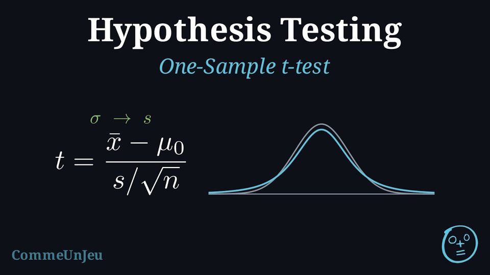
The t-test is one of the most commonly used statistical tests. It is used to determine if there is a significant difference between means, especially when the population variance is unknown and the sample size is small ($n < 30$).

Report an error

Definition — One-Sample t-test Formula

The one-sample t-test compares the mean of a single sample ($\bar{x}$) to a known or hypothesized population mean ($\mu_0$).
It is used when:

The data come from a random sample of quantitative (continuous) values.
The population follows a normal distribution (or the sample size is large, commonly $n \geq 30$, so that the distribution of $\bar{x}$ is approximately normal).
The population standard deviation $\sigma$ is unknown (we use the unbiased sample standard deviation $s = s_{n-1}$, the $s_x$ key of calculators).

The test statistic $t$ is calculated as:$$ t = \frac{\bar{x} - \mu_0}{s / \sqrt{n}} $$

Method — Steps for a One-Sample t-test using Calculator

Step 1: Write the Hypotheses
- $H_0: \mu = k$ (The population mean equals a specific value $k$).
- $H_1: \mu \neq k$ (or $\mu < k$, $\mu > k$ depending on the question).
Step 2: Enter data into GDC
- Enter the data into List 1 (or use summary statistics $\bar{x}, s, n$).
- Select T-Test (or 1-Sample t-test).
- Enter the value of $\mu_0$ (from $H_0$).
Step 3: Decision Rule
Compare the p-value with the significance level $\alpha$.
- If $p\text{-value} < \alpha$: Reject $H_0$.
- If $p\text{-value} \geq \alpha$: Fail to reject $H_0$.
Step 4: Conclusion
State whether there is sufficient evidence to support the alternative hypothesis, in context.

Example

A factory produces screws with a target length of 50 mm. A quality control manager takes a random sample of 15 screws and finds a mean length of 49.8 mm with a standard deviation of 0.5 mm.
Conduct a t-test at the 5$\pourcent$ significance level to see if the mean length is different from 50 mm.

Answer

Step 1: Hypotheses
- $H_0: \mu = 50$ (The mean is 50 mm).
- $H_1: \mu \neq 50$ (The mean is different from 50 mm).
Step 2: Calculator
Using GDC with inputs: $\mu_0=50, \bar{x}=49.8, s_x=0.5, n=15$. $$ t \approx -1.549 $$ $$ p\text{-value} \approx 0.144 $$
Step 3: Decision
$0.144 > 0.05$. Since $p > \alpha$, we fail to reject $H_0$.
Step 4: Conclusion
There is insufficient evidence at the 5$\pourcent$ level to claim that the mean length of the screws is different from 50 mm.

Skills to practice

Conducting One-Sample t-tests

II.2 The Two-Sample t-test

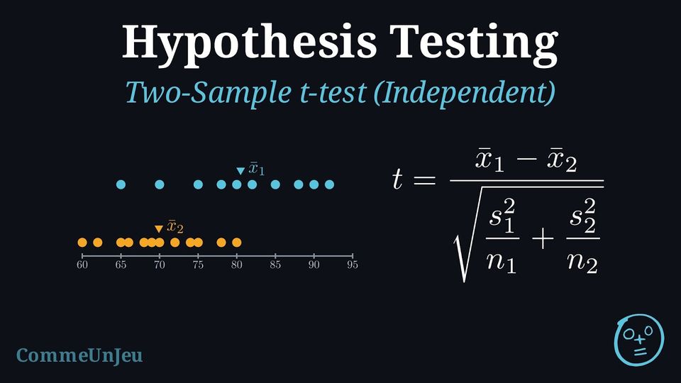
Definition — Two-Sample t-test Formula

The two-sample t-test compares the means of two independent groups to see if they are significantly different.The test statistic is given by:$$ t = \frac{\bar{x}_1 - \bar{x}_2}{\sqrt{\frac{s_1^2}{n_1} + \frac{s_2^2}{n_2}}} $$ Where:

$\bar{x}_1, \bar{x}_2$ are the sample means.
$s_1^2, s_2^2$ are the sample variances.
$n_1, n_2$ are the sample sizes.

Assumptions: both groups are independent random samples from (approximately) normal populations, or both sample sizes are large. The calculator computes the degrees of freedom of this statistic automatically.

Definition — Pooled Two-Sample t-test

When the two independent samples come from normal populations with the same unknown variance $\sigma^2$, both samples estimate this one variance, and the pooled estimate combines them, each weighted by its number of degrees of freedom: $$\textcolor{colordef}{s_p^2 = \dfrac{(n_1 - 1)\,s_1^2 + (n_2 - 1)\,s_2^2}{n_1 + n_2 - 2}},$$ where $s_1^2$ and $s_2^2$ are the unbiased sample variances (computed with $n - 1$, the $s_x$ key of calculators squared). The pooled two-sample $t$-test of $H_0 : \mu_1 = \mu_2$ uses the statistic $$\textcolor{colordef}{t = \dfrac{\bar{x}_1 - \bar{x}_2}{s_p\sqrt{\dfrac{1}{n_1} + \dfrac{1}{n_2}}}},$$ which, when $H_0$ is true, follows the $t$-distribution with $n_1 + n_2 - 2$ degrees of freedom. On a calculator, it is the 2-sample $t$-test with the setting Pooled: Yes. The equal-variance assumption is made when the question states it, when a course or an examination sets it as the convention, or when the context makes it a reasonable modelling choice (two groups measured in the same way, with close sample standard deviations, which support it without proving it); otherwise, the unpooled statistic of the two-sample $t$-test is used.

Example

Seedlings of the same variety are grown with two nutrient solutions, $A$ and $B$, in two independent random samples. Their heights after four weeks, in cm, are:

solution $A$: $24.1$, $25.3$, $23.8$, $26.0$, $24.7$, $25.5$;
solution $B$: $22.9$, $23.5$, $24.0$, $22.4$, $23.8$, $23.1$, $24.2$.

Assuming that the heights are normally distributed with the same variance for both solutions, test at the $5\pourcent$ significance level whether solution $A$ gives a greater mean height.

Answer

Let $\mu_A$ and $\mu_B$ be the mean heights, in cm, with each solution.

$H_0 : \mu_A = \mu_B$ and $H_1 : \mu_A > \mu_B$ (one-tailed).
Normal populations with a common variance: pooled two-sample $t$-test at $\alpha = 0.05$.
From the lists: $\bar{x}_A = 24.9$, $s_A^2 = 0.724$ ($n_A = 6$); $\bar{x}_B \approx 23.414$, $s_B^2 \approx 0.4181$ ($n_B = 7$). $$\begin{aligned}[t] s_p^2 &= \frac{(n_A - 1)\,s_A^2 + (n_B - 1)\,s_B^2}{n_A + n_B - 2} && \text{(pooled estimate)} \\ &\approx \frac{5 \times 0.724 + 6 \times 0.4181}{11} \approx 0.5571, \\ t &= \frac{\bar{x}_A - \bar{x}_B}{s_p\sqrt{\frac{1}{n_A} + \frac{1}{n_B}}} && \text{(pooled statistic)} \\ &\approx \frac{24.9 - 23.414}{0.7464 \times 0.5563} \approx 3.58, \end{aligned}$$ with $6 + 7 - 2 = 11$ degrees of freedom. The calculator (2-sample $t$-test, Pooled: Yes, $\mu_1 > \mu_2$) gives $t \approx 3.578$ and $p\text{-value} \approx 0.00217$.
$0.00217 \leq 0.05$: reject $H_0$.
At the $5\pourcent$ level, the data show that solution $A$ gives taller seedlings on average.

Skills to practice

Conducting Pooled Two-Sample t-tests

III Chi-squared Tests

III.1 The Chi-squared Test for Independence

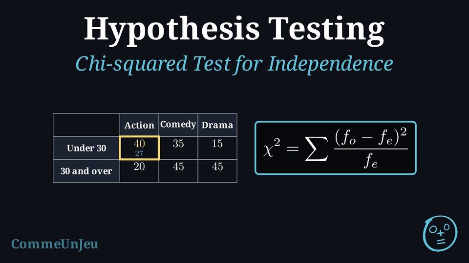
Every test so far has compared numerical measurements, such as means. The chi-squared test extends hypothesis testing to categorical data. In this sense it is the categorical analogue of correlation: a correlation coefficient measures the association between two numerical variables, while the chi-squared test of independence asks whether two categorical variables are associated.

Report an error

Definition — Two-Way Table of Counts

Two qualitative variables are observed on the same population of $N$ individuals. The two-way table of counts has one row for each category of the first variable and one column for each category of the second; the cell at row $A$ and column $B$ holds the count of the individuals that have both categories $A$ and $B$, written $n(A \cap B)$.

The last column holds the row totals: $n(A)$ is the number of individuals of category $A$.
The last row holds the column totals: $n(B)$ is the number of individuals of category $B$.
The bottom-right cell holds the grand total $N$, which is the sum of the row totals and the sum of the column totals.

The Chi-squared ($\chi^2$) test for independence determines if there is a significant association between two categorical variables. It compares the observed frequencies in a contingency table to the frequencies we would expect if the variables were completely independent.

Report an error

Definition — Observed and Expected Frequencies

Observed Frequencies ($f_o$): The actual data collected and recorded in a contingency table.
Expected Frequencies ($f_e$): The theoretical counts calculated assuming the variables are independent.

The formula for the expected frequency of a cell is:$$ f_e = \frac{\text{Row Total} \times \text{Column Total}}{\text{Grand Total}} $$

Definition — Chi-squared Statistic

The test statistic $\chi^2_{calc}$ measures the total deviation between observed and expected values:$$ \chi^2_{calc} = \sum \frac{(f_o - f_e)^2}{f_e} $$ The degrees of freedom ($df$) for a table with $r$ rows and $c$ columns is:$$ \mathrm{d}f = (r - 1)(c - 1) $$

Method — Steps for a Chi-squared Test

Step 1: Write the Hypotheses
- $H_0$: The variables are independent.
- $H_1$: The variables are not independent (associated).
Step 2: Enter data into GDC
- Enter the observed contingency table into a Matrix (e.g., Matrix A).
- Select $\chi^2$-Test (usually under Stat $\to$ Tests).
Step 3: Analyze Results
The calculator provides $\chi^2_{calc}$, the p-value, and the degrees of freedom ($df$).
Note: As a rule of thumb, all expected frequencies should be at least 5 for the test to be reliable.
Step 4: Conclusion
Compare the p-value to the significance level $\alpha$.
- If $p\text{-value} < \alpha$: Reject $H_0$ (Variables are dependent/associated).
- If $p\text{-value} \geq \alpha$: Fail to reject $H_0$ (No evidence of association).

Example

A survey asked 200 people about their preferred type of movie and their age group. The results are shown below:

	Action	Comedy	Drama
Under 30	40	35	15
30 and over	20	45	45

Test at the 5$\pourcent$ significance level whether age group and movie preference are independent.

Answer

Step 1: Hypotheses
$H_0$: Age group and movie preference are independent.
$H_1$: Age group and movie preference are not independent (they are associated).
Step 2: Calculator
Enter the $2 \times 3$ matrix into the calculator and run the $\chi^2$-Test.
- $\chi^2_{calc} \approx 21.1$
- $\mathrm{d}f = (2-1)(3-1) = 2$
- $p\text{-value} \approx 0.000026$ (about $2.6 \times 10^{-5}$)
Step 3: Conclusion
$0.000026 < 0.05$. Since $p < \alpha$, we reject $H_0$.
There is strong evidence to suggest that movie preference depends on age group.

Method — Deciding with a $\chi^2$ Critical Value

The statistic $\chi^2_{calc}$ is never negative, and it grows as the observed frequencies move away from the expected ones: only large values count against $H_0$, so a $\chi^2$ test is always upper-tailed. Its critical value $\chi^2_{crit}$ is the number such that $P(\chi^2 \geq \chi^2_{crit}) = \alpha$ for the $\chi^2$ distribution with the degrees of freedom $\nu$ of the test; it is read in a table or given in the question.

Expected frequencies: compute them, and check that each one is greater than $5$.
Statistic: $\chi^2_{calc} = \sum \dfrac{(f_o - f_e)^2}{f_e}$, by hand for a small table or with the calculator, and the degrees of freedom $\nu$.
Decision: reject $H_0$ if $\chi^2_{calc} \geq \chi^2_{crit}$; otherwise do not reject it. It is the same decision as rejecting when $p\text{-value} \leq \alpha$.

$\nu$	$1$	$2$	$3$	$4$	$5$	$6$	$9$
$\alpha = 0.10$	$2.706$	$4.605$	$6.251$	$7.779$	$9.236$	$10.645$	$14.684$
$\alpha = 0.05$	$3.841$	$5.991$	$7.815$	$9.488$	$11.070$	$12.592$	$16.919$
$\alpha = 0.01$	$6.635$	$9.210$	$11.345$	$13.277$	$15.086$	$16.812$	$21.666$

Example

A café asks $150$ customers whether they prefer coffee or tea, and notes their age group.

	Coffee	Tea
Under $40$	$45$	$30$
$40$ and over	$25$	$50$

By computing the expected frequencies and the statistic by hand, test at the $5\pourcent$ significance level whether the preferred drink is independent of the age group, using the critical value.

Answer

$H_0$: the preferred drink is independent of the age group; $H_1$: it is not.
The row totals are $75$ and $75$, the column totals $70$ (coffee) and $80$ (tea), the grand total $150$. For the cell “under $40$, coffee”: $$f_e = \frac{\text{row total} \times \text{column total}}{\text{grand total}} = \frac{75 \times 70}{150} = 35,$$ and likewise $40$ for “under $40$, tea”, $35$ and $40$ for the second row: all greater than $5$.
Every cell is $10$ away from its expected frequency: $$\begin{aligned}[t] \chi^2_{calc} &= \sum \frac{(f_o - f_e)^2}{f_e} && \text{(statistic)} \\ &= \frac{10^2}{35} + \frac{10^2}{40} + \frac{10^2}{35} + \frac{10^2}{40} \\ &\approx 2.857 + 2.5 + 2.857 + 2.5 \approx 10.71, \end{aligned}$$ with $\nu = (2 - 1)(2 - 1) = 1$.
At $\alpha = 0.05$ and $\nu = 1$, $\chi^2_{crit} = 3.841$. Since $10.71 > 3.841$, reject $H_0$ (the calculator gives $p\text{-value} \approx 0.00106$, the same decision).
At the $5\pourcent$ level, the preferred drink depends on the age group: the younger customers lean towards coffee, the older towards tea.

Skills to practice

Deciding with a Critical Value
Computing Expected Frequencies and Degrees of Freedom
Conducting Chi-squared Tests for Independence

III.2 The Chi-squared Goodness of Fit Test

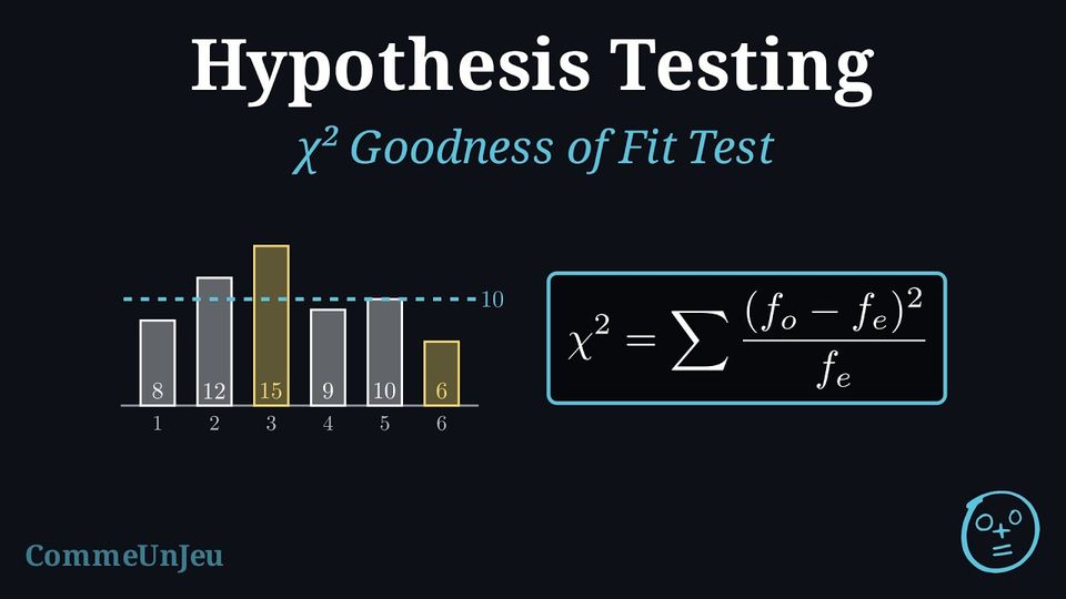
The Goodness of Fit (GOF) test is used to determine whether a variable is likely to come from a specified distribution (such as Uniform, Binomial, Normal, or a specific ratio). It compares the observed data with what we would expect theoretically.

Report an error

Definition — Goodness of Fit Statistic

The test uses the same $\chi^2$ statistic formula:$$ \chi^2_{calc} = \sum \frac{(f_o - f_e)^2}{f_e} $$ However, the degrees of freedom ($df$) calculation depends on the distribution:$$ \mathrm{d}f = k - 1 - m $$ Where:

$k$ is the number of categories (bins).
$m$ is the number of population parameters estimated from the sample data (e.g., if you calculate mean and standard deviation from the sample to fit a Normal distribution, $m=2$).

Method — Steps for a GOF Test

Step 1: Hypotheses
- $H_0$: The data follow the specified distribution.
- $H_1$: The data do not follow the specified distribution.
Step 2: Expected Frequencies
Calculate the expected frequency for each category: $$ f_e = n \times P(\text{category}) $$ (As for the independence test, all expected frequencies should be at least 5 for the $\chi^2$ approximation to be reliable.) Note: Usually done in List 2 of the GDC.
Step 3: Calculator
- Enter observed values in List 1 ($f_o$).
- Enter expected values in List 2 ($f_e$).
- Select $\chi^2$ GOF Test.
- Enter the correct $df$.
Step 4: Conclusion
Compare p-value to $\alpha$ and interpret in context.

Example

A die is rolled 60 times. The results are:

Outcome	1	2	3	4	5	6
Frequency	8	12	15	9	10	6

Test at the 5$\pourcent$ level if the die is fair (Uniform distribution).

Answer

Hypotheses:
$H_0$: The die is fair (Uniform distribution).
$H_1$: The die is not fair.
Expected Frequencies:
Total $n=60$. If fair, $P(X=k) = 1/6$. $$ f_e = 60 \times \frac{1}{6} = 10 \quad \text{for all outcomes} $$
Calculator / Working:
$L_1: \{8, 12, 15, 9, 10, 6\}$
$L_2: \{10, 10, 10, 10, 10, 10\}$ $$ \chi^2_{calc} = \sum \frac{(f_o - f_e)^2}{f_e} = \frac{(8-10)^2}{10} + \frac{(12-10)^2}{10} + \cdots + \frac{(6-10)^2}{10} = 5.0 $$ Degrees of freedom: $\mathrm{d}f = k - 1 = 6 - 1 = 5$ (no parameters estimated).
$p\text{-value} \approx 0.416$.
Conclusion:
$0.416 > 0.05$. We fail to reject $H_0$: there is insufficient evidence at the 5\,$\pourcent$ level to conclude the die is unfair.

Skills to practice

Finding Expected Frequencies for a Goodness of Fit
Conducting Chi-squared Goodness of Fit Tests

IV Going further

Skills to practice

Solving Problems with Hypothesis Tests
Quiz

\(\nu\)	\(1\)	\(2\)	\(3\)	\(4\)	\(5\)	\(6\)	\(9\)
\(\alpha = 0.10\)	\(2.706\)	\(4.605\)	\(6.251\)	\(7.779\)	\(9.236\)	\(10.645\)	\(14.684\)
\(\alpha = 0.05\)	\(3.841\)	\(5.991\)	\(7.815\)	\(9.488\)	\(11.070\)	\(12.592\)	\(16.919\)
\(\alpha = 0.01\)	\(6.635\)	\(9.210\)	\(11.345\)	\(13.277\)	\(15.086\)	\(16.812\)	\(21.666\)

	Coffee	Tea
Under \(40\)	\(45\)	\(30\)
\(40\) and over	\(25\)	\(50\)