International Baccalaureate · DP 1: Applications and Interpretation SL
Sampling and Data
I
Statistical Investigations and Data
I.1
The Statistical Investigation Process
Recappreviously studied — click to reread
Statistics are all around us, from sports averages to news reports about the weather.
- A basketball player averages 14.6 points per game.
- Last year was the hottest year on record since 1897.
Definition — Statistics
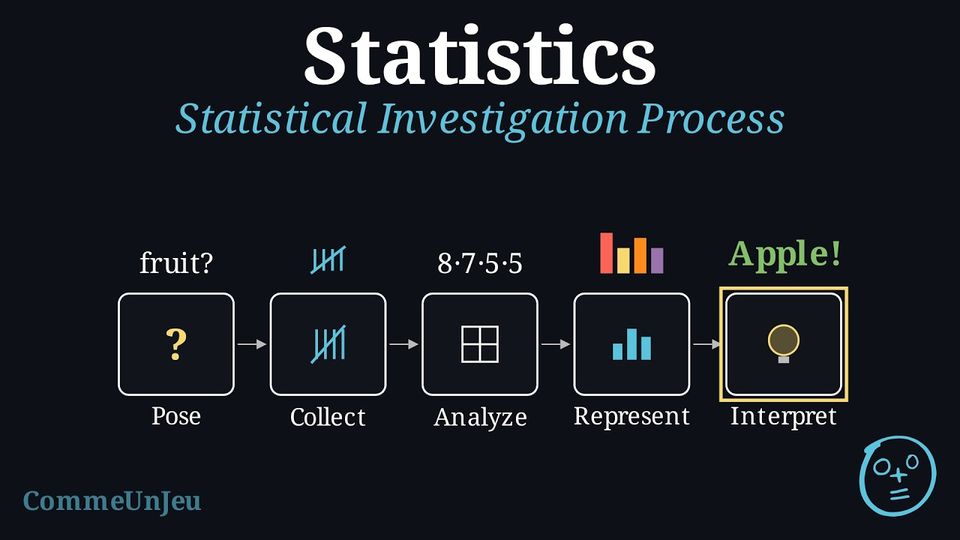
Statistics is the science of designing investigations and then collecting, organising, analysing and interpreting data to answer a specific question. Method — The Statistical Investigation Process
A rigorous statistical investigation follows five key steps: - Pose the Question: Define a clear research problem, identifying the target population and the variables to be investigated.
- Collect Data: Design a data collection plan and gather information using an appropriate sampling method.
- Analyse Data: Calculate relevant descriptive statistics to summarise the data numerically. This includes calculating relative frequencies (percentages), measures of central tendency (mean, median, mode), and measures of spread (standard deviation, IQR).
- Represent Data: Structure the raw data into tables (e.g., a frequency table showing counts/tallies) and create initial visual representations (e.g., histograms, bar charts) to see the distribution.
- Interpret and Conclude: Make inferences from the analysis, provide a conclusion that answers the initial question, and critically evaluate the limitations of the investigation.
Skills to practice
- Identifying the Steps of an Investigation
I.2
Populations and Types of Data
Recappreviously studied — click to reread
Definition — Statistical Question
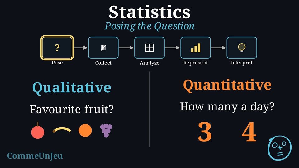
A statistical question is a clear, focused question that is answered by collecting and analysing data, and whose answers vary: from one person or one object to another, the answer is not always the same. Example
We investigate the statistical question: “What is the favourite school subject of the students at our school?” Definition — Population
In statistics, a population is the complete set of all individuals, items, or events that share a common, well-defined characteristic of interest for an investigation. Example
For our problem, the population is all students at our school. Asking every student is impractical, so the data used in the next steps comes from a sample of 25 students (see Census vs. Survey below). Definition — Data
Data is the information we collect, like numbers, words, measurements, or observations. Example
The data we collect will be the list of answers from each student, such as “Maths”, “Art”, “Science”, “Art”, “Sport”, etc. Definition — Types of Variables
A variable is a characteristic of an individual in the population that can take different values. Variables are classified into two main types: - Qualitative Variable (Categorical): Represents characteristics that belong to a category or group (e.g., eye colour, type of car, favourite subject).
- Quantitative Variable (Numerical): Represents characteristics that can be counted or measured numerically. These can be further divided into:
- Discrete: The variable can only take specific, separate numerical values (often integers). It is typically data that is counted.
- Continuous: The variable can take any numerical value within a given range. It is typically data that is measured.
Example
We classify some variables from a student survey: - The variable “Favourite Subject” is qualitative.
- The variable “Number of siblings” is a discrete quantitative variable, as the answers can only be integers (0, 1, 2, ...).
- The variable “Height in centimetres” is a continuous quantitative variable, as a student's height could be any value within a range (e.g., 165.2 cm, 165.25 cm, etc.).
Skills to practice
- Sorting Variables into Three Types
II
Collecting Data by Sampling
II.1
Census or Sample
Recappreviously studied — click to reread
When we conduct an investigation, we must decide who to collect data from. Do we ask everyone in the population, or just a smaller group?
Definition — Census vs. Survey
- A census collects data from every single member of the population. It gives the exact answer for the population, if everyone answers, but it can be very slow and expensive for large populations.
- A survey collects data from a smaller, manageable group taken from the population, called a sample (choosing this group is called sampling). It is much faster, but the sample must be chosen carefully to be representative of the whole population.
Example
An investigation asks: “What is the favourite subject of students at this school?”If every student in the school is asked, is it a census or a survey?
It is a census because data are collected from the entire population (all students in the school).
Example
An investigation asks: “What is the favourite subject of students at this school?”If only the students of one Maths class are asked, is it a census or a survey?
It is a survey because data are only collected from a small sample (one Maths class) of the total population (the whole school).
Definition — Representative Sample
A sample is representative when it reflects the whole population: the different groups inside the population appear in the sample in about the same proportions as in the population. A conclusion drawn from a representative sample can reasonably be extended to the whole population. A sample that is biased leans toward one type of answer and does not reflect the population, so its conclusion cannot be trusted. Skills to practice
- Choosing between a Census and a Sample
II.2
Parameters and Statistics
Definition — Parameter and Statistic
A parameter is a number that describes a whole population, for example the mean height of all the students of a school. A statistic is a number calculated from the data of a sample, for example the mean height of the \(50\) students of a sample. - A parameter is fixed, but it is usually unknown: a sample alone does not give it exactly.
- A statistic is known as soon as the sample has been measured, but another sample would usually give a slightly different value. A statistic is used to estimate a parameter.
Example
A sports club has \(1{,}850\) members. It asks \(200\) members, chosen at random, whether the club should close later in the evening, and \(124\) of them answer yes.Identify the population, the sample, the statistic and the parameter it estimates.
- Population: the \(1{,}850\) members of the club. Sample: the \(200\) members who were asked.
- Statistic: the proportion of the sample who answer yes, $$\frac{124}{200} = 0.62 = 62\pourcent.$$
- Parameter: the proportion of all \(1{,}850\) members who want the club to close later. It is unknown, since only \(200\) members were asked; the statistic \(62\pourcent\) is its estimate.
Skills to practice
- Distinguishing a Parameter from a Statistic
II.3
Sampling Methods
Recappreviously studied — click to reread
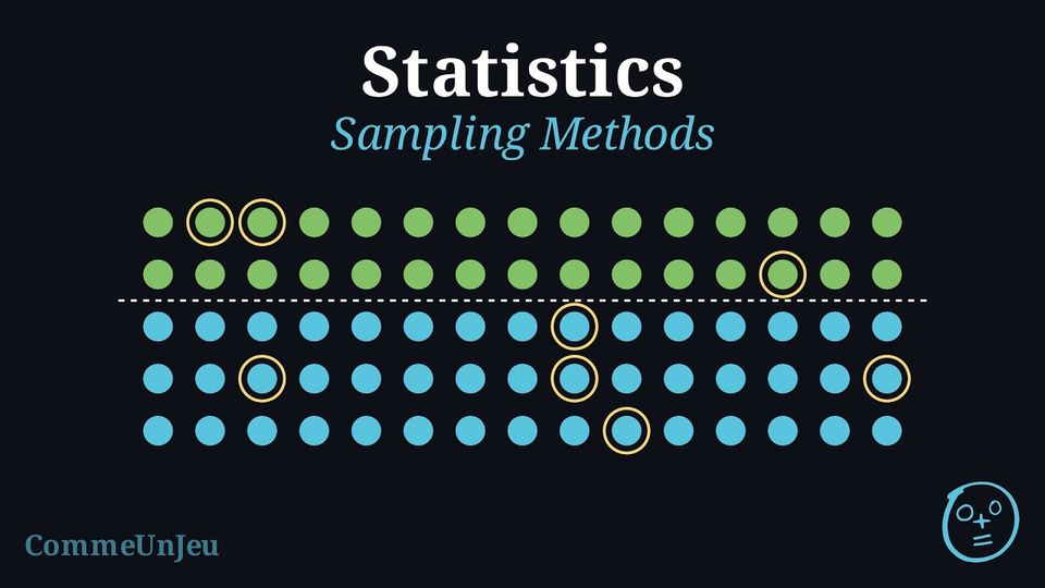
When conducting a survey, our goal is to select a sample that is representative of the entire population. The method used to select this sample is critical. A poorly chosen method can lead to a biased sample, where certain parts of the population are over- or under-represented, making the conclusions invalid.
Definition — Probability Sampling
In probability sampling, every member of the population has a known, non-zero chance of being selected. In these methods, chance — not the surveyor's choices — decides who is selected. - Simple Random Sampling: Every member has an equal chance of selection (more precisely, every possible group of \(n\) individuals has the same chance of being the chosen sample).
Example: Drawing 3 names from a hat containing all 30 students' names. - Systematic Sampling: Members are selected at a regular interval (\(k\)) from an ordered list, starting from a random point between 1 and \(k\).
Example: Surveying every 20th customer entering a store, starting from a randomly chosen one. - Stratified Sampling: The population is divided into subgroups (strata), and a simple random sample is taken from each stratum, often proportional to its size.
Example: A school with 40\(\pourcent\) boys and 60\(\pourcent\) girls takes a random sample of 40 boys and 60 girls.
Definition — Non-Probability Sampling
In non-probability sampling, the selection of the sample is not random and is often based on the researcher's judgement or convenience. These methods are highly prone to bias. - Convenience Sampling: Selecting the most easily accessible members of the population.
Example: Surveying only your own friends about a school-wide issue. - Quota Sampling: Similar to stratified sampling, but individuals within each subgroup are selected non-randomly (e.g., by convenience) until a quota is met.
Example: A researcher needs 30 male and 30 female participants and simply surveys the first 30 of each gender they meet.
Skills to practice
- Identifying Sampling Methods
II.4
Sizing a Sample
Method — Sizing a Stratified or a Systematic Sample
A sample of size \(n\) is to be taken from a population of size \(N\). - Stratified sample: each stratum receives the same share of the sample as its share of the population. A stratum of size \(N_i\) therefore receives $$n_i = \frac{N_i}{N} \times n \text{ members.}$$ Round each \(n_i\) to the nearest whole number and check that the sizes add up to \(n\). If the total is too large by \(d\), lower by \(1\) the \(d\) sizes that rounding increased the most; if it is too small by \(d\), raise by \(1\) the \(d\) sizes that rounding decreased the most. The members of each stratum are then chosen at random. If they are chosen for convenience instead, with the same sizes, the sample is a quota sample.
- Systematic sample: the members of the population are numbered from \(1\) to \(N\) in a list, and the sampling interval is $$k = \frac{N}{n},$$ rounded to a whole number when \(N\) is not a multiple of \(n\) (the sample then has about \(n\) members; the method suits a sample that is small compared with the population). A random start \(r\) is drawn between \(1\) and \(k\), for example with a random-number generator, and all the members numbered \(r\), \(r + k\), \(r + 2k\), … up to \(N\) are selected: each member has the same chance, \(\frac{1}{k}\), of being selected, and the \(m\)-th member selected is number \(r + (m - 1)k\). If the list follows a pattern that repeats every \(k\) members, a systematic sample can be biased: the list must first be checked for such a pattern.
Example
A sports centre has \(820\) members in four activities: swimming \(355\), fitness \(192\), climbing \(152\) and badminton \(121\). The manager wants a stratified sample of \(80\) members, stratified by activity.Find the number of members to select in each activity.
Each activity receives \(n_i = \dfrac{N_i}{820} \times 80\) members. For swimming, $$n_{1} = \frac{355}{820} \times 80 \approx 34.63,$$ and the same computation gives the other sizes:
The rounded sizes add up to \(81\), one too many. Rounding increased swimming the most (\(34.63 \to 35\), an increase of \(0.37\), against \(0.27\), \(0.17\) and \(0.20\)), so swimming is lowered to \(34\). The manager selects at random \(34\) swimmers, \(19\) fitness members, \(15\) climbers and \(12\) badminton players: \(34 + 19 + 15 + 12 = 80\).
| Activity | \(N_i\) | \(\frac{N_i}{820} \times 80\) | Rounded | Final size |
| Swimming | \(355\) | \(34.63\) | \(35\) | \(\mathbf{34}\) |
| Fitness | \(192\) | \(18.73\) | \(19\) | \(19\) |
| Climbing | \(152\) | \(14.83\) | \(15\) | \(15\) |
| Badminton | \(121\) | \(11.80\) | \(12\) | \(12\) |
| Total | \(820\) | \(80\) | \(81\) | \(80\) |
Example
A cinema sold \(2{,}400\) tickets last week, numbered from \(1\) to \(2{,}400\). To check the ticket machines, \(120\) tickets are examined with a systematic sample. A random-number generator gives the start \(r = 13\).Find the sampling interval, the numbers of the first three tickets selected and the number of the last one.
The sampling interval is $$k = \frac{N}{n} = \frac{2400}{120} = 20,$$ and the start \(r = 13\) was drawn between \(1\) and \(20\). The tickets selected are numbered \(13\), \(13 + 20 = 33\), \(33 + 20 = 53\), and so on. The last ticket selected, in position \(m = 120\), is number $$\begin{aligned}[t] r + (120 - 1)k &= 13 + 119 \times 20 && \text{(position } m = 120\text{)}\\
&= 13 + 2380\\
&= 2393. \end{aligned}$$ Check: \(2393 \leq 2400\), and the next number, \(2413\), is beyond the list. Every ticket had the same chance, \(\dfrac{1}{20}\), of being selected, because the start was drawn at random.
Skills to practice
- Selecting a Systematic Sample
- Calculating Stratum Sizes
III
Errors in Sampling
III.1
Sampling Error and Bias
Recappreviously studied — click to reread
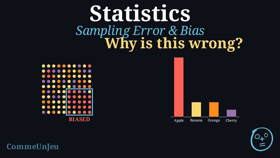
One of the most common ways to collect information about a large group is to use a sample. For a sample to be meaningful, it must fairly represent the entire population. Two key challenges in sampling are avoiding bias and choosing a sample size that is large enough to capture the population’s diversity.
- Selection bias: A famous example of biased sampling is the Literary Digest poll before the 1936 US presidential election. The magazine sent millions of surveys using telephone books and car registration lists. But during the Great Depression, many people could not afford phones or cars. This led to a sample heavily biased towards wealthier citizens, who at the time were more likely to vote Republican. Because of this bias, the poll incorrectly predicted a landslide win for Alfred Landon, while Franklin D. Roosevelt actually won by a wide margin.
- Sample size: In a school of \(1\,000\) students, \(500\) walk to school, that is \(50\pourcent\). Two groups of students are chosen at random and asked. In a sample of \(10\) students, \(7\) walk to school, that is \(70\pourcent\); in a sample of \(200\) students, \(104\) walk, that is \(52\pourcent\). Both samples are chosen fairly, but the small one is far from the true \(50\pourcent\), by chance alone: with \(10\) students, one walker more or fewer changes the result by \(10\pourcent\); with \(200\) students, by only \(0.5\pourcent\).
Definition — Sampling Error
A result calculated from a sample usually differs from the true value for the entire population. Sampling error is the part of that difference that comes from chance alone. It exists simply because a sample is a part of the whole, not the whole itself, and because the individuals chosen by chance will usually differ somewhat from the population as a whole. Definition — Selection Bias
Selection bias is a systematic error that occurs when the method of selecting a sample causes it to be unrepresentative of the population. Unlike random sampling error, bias pushes the results in a specific direction and does not disappear just by increasing the sample size. Definition — Common Sources of Bias
Three ways of building a sample often make it biased: - Convenience: choosing the people who are easiest to reach. Example: to learn the favourite sport of a town, only the people leaving a swimming pool are asked — swimmers are over-represented.
- Voluntary response: letting people decide for themselves whether to answer. Example: a magazine prints a survey and only the readers who feel strongly send it back.
- Undercoverage: leaving part of the population out of the sample completely. Example: to survey a whole school, only the students who own a smartphone are asked — those without one are never reached.
Example
An investigation asks: “What is the favourite subject of the students at this school?” To collect data, only the students of one maths class are surveyed.This is a biased sample.
- The population is all the students of the school.
- The sample is only the students of this maths class.
Definition — Measurement Error
Measurement error refers to inaccuracies in the data that arise during the collection process itself. Common causes include: - Poorly worded questions: Ambiguous, “double-barrelled” or leading questions that confuse or influence the respondent.
- Response bias: Respondents provide inaccurate answers due to social desirability (wanting to appear favourable) or misunderstanding the question.
Example
A survey asks students: “Don't you agree that amazing Mathematics is the most important subject for your future?”Identify the source of error.
This is a source of measurement error. The question is leading for two reasons:
- It uses the biased adjective “amazing” to describe mathematics.
- It uses the phrase “Don't you agree”, which pressures the respondent to answer “Yes”.
Definition — Total Survey Error
The total survey error is the difference between a result calculated from the sample and the true value for the population. It is composed of two types of error: - Sampling Error: Natural, random variation due to observing a sample instead of the whole population.
- Non-Sampling Error: Errors arising from the survey design or execution — selection bias, measurement, recording or non-response errors (they can be systematic or random).
Method — Reducing Error in Sampling
To ensure a survey's results are as accurate as possible, statisticians use two main strategies: - Use Random Sampling: To reduce selection bias, every member of the population should have an equal chance of being chosen for the sample. This is the foundation of reliable surveying (though a good design requires more than equal chances alone).
- Increase the Sample Size: As the sample size gets larger, it is more likely to accurately reflect the diversity of the population, and the random sampling error generally decreases. However, increasing the sample size alone does not remove selection bias if the method of selection is already flawed.
Skills to practice
- Explaining the Bias of a Sample
III.2
Non-Response and Missing Data
Definition — Non-Response Error
A non-response error occurs when some of the members chosen for a sample do not answer — they refuse, cannot be reached or do not return the questionnaire — and those who answer differ from those who do not in what the survey measures. The response rate is $$\text{response rate} = \frac{\text{number of members who answered}}{\text{number of members chosen for the sample}},$$ often written as a percentage. A low response rate is a warning: the answers then come from the members who chose to reply, and the results may be biased even when the sample itself was chosen at random. Sending more questionnaires to the same kind of people does not remove this bias. Example
An online shop emails a satisfaction questionnaire to \(800\) customers chosen at random; \(248\) of them reply.Calculate the response rate, and explain why the results may be biased even though the \(800\) customers were chosen at random.
$$\text{response rate} = \frac{248}{800} = 0.31 = 31\pourcent.$$ More than two customers out of three did not reply. Customers who reply to a satisfaction questionnaire are often those with a strong opinion, very satisfied or very dissatisfied, so the \(248\) replies may not represent the \(800\) customers chosen, and even less all the customers of the shop. The random choice of the \(800\) protects against selection bias, not against non-response error. Reminders or a shorter questionnaire can raise the response rate, and contacting again a random part of the non-respondents gives an idea of whether they answer differently.
Method — Dealing with Missing Data and Recording Errors
Before a data set is analysed, it is checked. - Look for impossible or suspicious values: a value outside the possible range (a person's height of \(17.5\)~m, a mark of \(45\) out of \(20\)), a decimal point or a unit typed wrongly, the same record entered twice.
- Correct a recording error only when the true value is certain, for example from the original form. Otherwise, remove the value and treat it as missing.
- Do not replace a missing value by zero or by a guessed value: each statistic is calculated from the values that are available, and the number of values used, \(n\), is stated.
- Report what was removed, and ask why values are missing: if the missing values are likely to differ from the others, the statistics calculated from the available values may be biased, as with a non-response error.
Example
A coach records the \(100\) m times, in seconds, of the \(12\) athletes of a club. One athlete was absent (–), and one time was typed as \(1.34\); the original sheet has been lost. | \(13.2\) | \(12.8\) | \(14.1\) | – | \(13.5\) | \(1.34\) |
| \(12.9\) | \(13.7\) | \(14.4\) | \(13.0\) | \(13.8\) | \(12.6\) |
Cleaning. A time of \(1.34\) s for \(100\) m is impossible, and the true value cannot be recovered: it is removed. The absent athlete has no time: that value is missing, not \(0\). There remain \(n = 10\) usable times.
Mean. $$\begin{aligned}[t] \bar{x} &= \frac{13.2 + 12.8 + 14.1 + 13.5 + 12.9 + 13.7 + 14.4 + 13.0 + 13.8 + 12.6}{10} && \text{(the } n = 10 \text{ usable times)}\\ &= \frac{134.0}{10}\\ &= 13.4 \text{ s}. \end{aligned}$$ Keeping \(1.34\) and counting the absence as \(0\) would give \(\dfrac{135.34}{12} \approx 11.3\) s, a mean faster than every one of the ten usable times. The mean \(13.4\) s is that of the \(10\) athletes whose times are known, and the report states that it is based on \(10\) of the \(12\) athletes.
Mean. $$\begin{aligned}[t] \bar{x} &= \frac{13.2 + 12.8 + 14.1 + 13.5 + 12.9 + 13.7 + 14.4 + 13.0 + 13.8 + 12.6}{10} && \text{(the } n = 10 \text{ usable times)}\\ &= \frac{134.0}{10}\\ &= 13.4 \text{ s}. \end{aligned}$$ Keeping \(1.34\) and counting the absence as \(0\) would give \(\dfrac{135.34}{12} \approx 11.3\) s, a mean faster than every one of the ten usable times. The mean \(13.4\) s is that of the \(10\) athletes whose times are known, and the report states that it is based on \(10\) of the \(12\) athletes.
Skills to practice
- Cleaning a Data Set
- Judging Non-Response and Missing Answers
IV
Organising and Displaying Data
IV.1
Frequency Tables
Recappreviously studied — click to reread
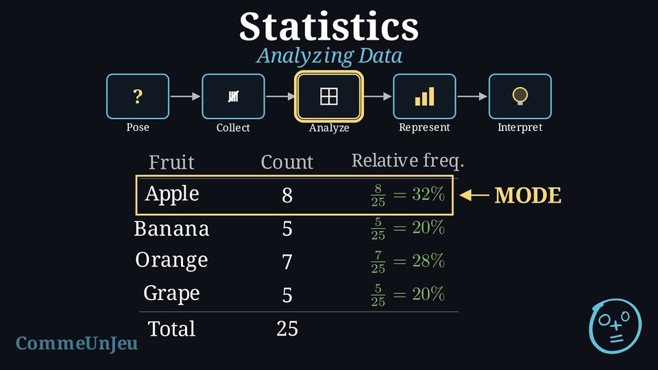
Definition — Frequency and Relative Frequency
The frequency (or count) of a category is how many times that category appears in our data.Relative frequency is the proportion of the data that falls into a category. We can write it as a fraction, a decimal, or a percentage. $$ \text{Relative frequency (in }\pourcent\text{)} = \frac{\text{Frequency}}{\text{Total number of data values}} \times 100\pourcent $$
Method — Creating a Frequency Table
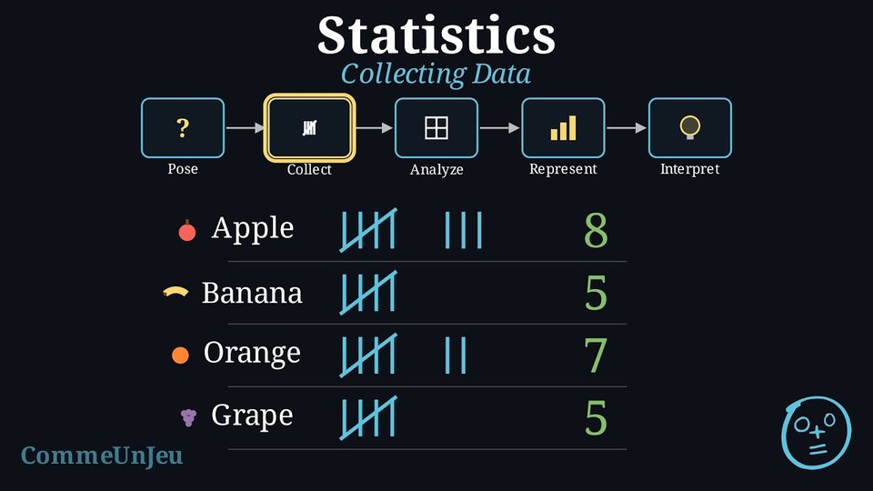
To organise our data, we use a frequency table. We use tally marks to count the frequency for each category. Then, we can calculate the relative frequency.Here is the data for the “Favourite Subject” survey of 25 students, organised into a frequency table:
| Subject | Tally Marks | Frequency (Count) | Relative Frequency |
| Maths | 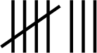 | 8 | \(8/25 = 32\pourcent\) |
| Science |  | 5 | \(5/25 = 20\pourcent\) |
| Sport |  | 7 | \(7/25 = 28\pourcent\) |
| Art | | 5 | \(5/25 = 20\pourcent\) |
| Total | 25 | 100\(\pourcent\) |
Skills to practice
- Calculating Relative Frequencies
IV.2
Histograms
Recappreviously studied — click to reread
The \(40\) pupils of a class noted how long, in minutes, their journey to school takes. The times were grouped:
In a bar chart, the bars stand apart, one per category. Here the times run on without a break from \(0\) to \(40\) minutes. How can a chart show that each group covers a whole interval of times?
| Time (min) | Number of pupils |
| \(0 \le t < 10\) | \(12\) |
| \(10 \le t < 20\) | \(16\) |
| \(20 \le t < 30\) | \(8\) |
| \(30 \le t < 40\) | \(4\) |
By rectangles that touch, drawn over a numbered axis: each rectangle stands on its whole interval, and its height gives the number of pupils. The four rectangles fill the axis from \(0\) to \(40\) without a gap, just as the times do. Such a chart is a histogram. 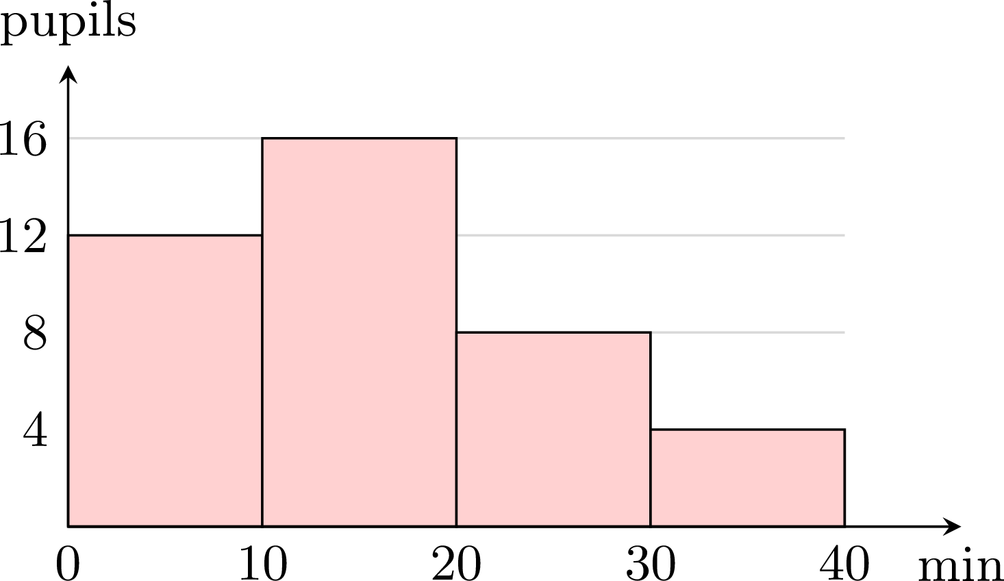
Definition — Classes and Histogram
When a quantity takes many different values (a time, a height, a mass…), the values are grouped into classes: intervals, here all of the same width, such as \(0 \le t < 10\) — from \(0\) included to \(10\) excluded, so that each value belongs to exactly one class. The frequency of a class is the number of values it contains. A histogram represents such a series: along a numbered horizontal axis, each class is drawn as a rectangle whose base is the class and whose height is its frequency. The rectangles touch, since the classes follow each other. Method — Drawing a Histogram
- Mark the horizontal axis with the bounds of the classes, evenly spaced, since the classes have the same width.
- Mark the vertical axis with the frequencies, from \(0\).
- Draw one rectangle per class: its base is the class, its height the frequency; the rectangles touch.
- Name the two axes, with their units.
Example
The masses of \(50\) apples picked in an orchard were grouped: | Mass (g) | Frequency |
| \(100 \le m < 120\) | \(6\) |
| \(120 \le m < 140\) | \(14\) |
| \(140 \le m < 160\) | \(18\) |
| \(160 \le m < 180\) | \(9\) |
| \(180 \le m < 200\) | \(3\) |
- Draw the histogram of this series.
- How many apples weigh at least \(140\) g? What percentage of the apples is that?
- The five classes have the same width, \(20\) g: the axis is marked from \(100\) to \(200\) in steps of \(20\), and each rectangle has the height of its frequency.
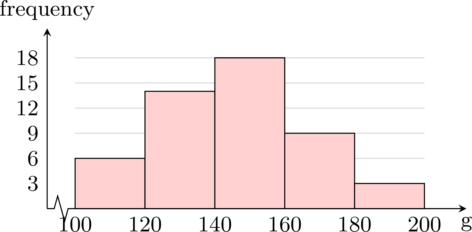
- The apples of at least \(140\) g are those of the last three classes: \(18 + 9 + 3 = 30\) apples, that is \(\dfrac{30}{50} = 0.6 = 60~\pourcent\) of the apples.
Example
The histogram shows the ages of the members of a sports club. 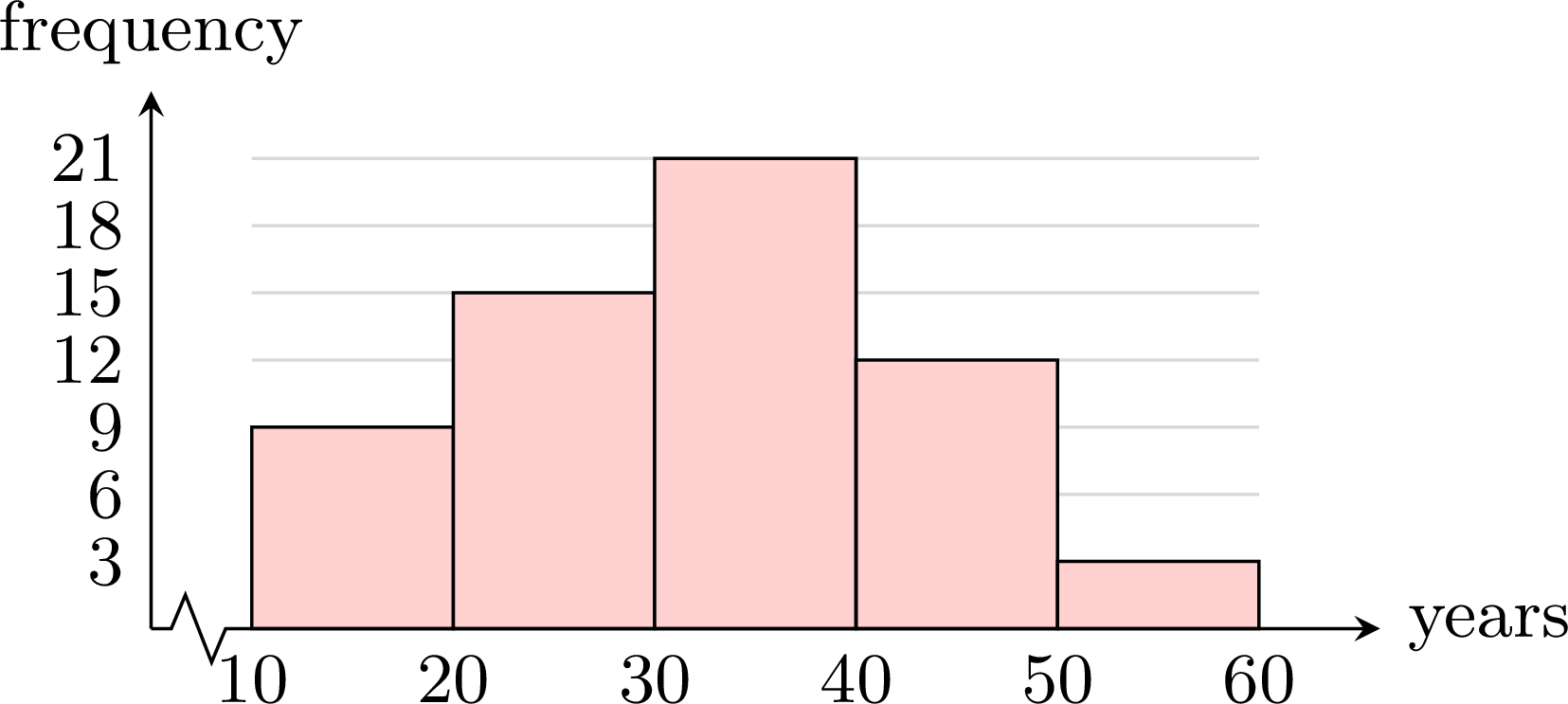
- What is the frequency of the class \(30 \le a < 40\)? How many members does the club have?
- What is the relative frequency of the members under \(30\)? Give it as a decimal, then as a percentage.
- What can be said about the range of the ages?
- The rectangle over \(30 \le a < 40\) rises to \(21\): \(21\) members. In total: \(9 + 15 + 21 + 12 + 3 = 60\) members.
- Under \(30\): the first two classes, \(9 + 15 = 24\) members out of \(60\). Relative frequency: \(\dfrac{24}{60} = 0.4\), that is \(40~\pourcent\).
- The exact ages are not known, only their classes: the youngest member is at least \(10\), the oldest under \(60\). The range is therefore less than \(60 - 10 = 50\) years — grouping the values hides its exact value.
Bar Chart or Histogram?
A bar chart shows separate categories or isolated values: its bars stand apart. A histogram shows classes that follow each other: its rectangles touch. With classes of the same width, the height of a rectangle reads directly as the frequency of its class.
Skills to practice
- Reading a Histogram
- Drawing and Using a Histogram
V
Going further
Skills to practice
- Solving Sampling Problems
- Solving Problems with Histograms
- Quiz
Jump to section