International Baccalaureate · DP 2: Applications and Interpretation HL

Revision: Functions and Modelling

⌚ ~35 min ▢ 4 blocks ✓ 16 exercises ➣ Prerequisites : Trigonometric Functions, Modelling

I Toolbox: Variation Models

Recappreviously studied — click to reread

Definition — Proportion with a Power

Let $n$ be a positive whole number and $k$ a nonzero number.

$y$ is directly proportional to $x^n$ when $y = kx^n$ for every pair of matching values. We write $y \propto x^n$. For $n = 2$, $y$ is proportional to the square of $x$; for $n = 3$, to the cube of $x$.
$y$ is inversely proportional to $x^n$ when $y = \dfrac{k}{x^n}$ for every pair of matching values, with $x \neq 0$. We write $y \propto \dfrac{1}{x^n}$. For $n = 2$, this is the inverse-square law.

For $n = 1$, these are direct proportion and inverse proportion.

Proposition — Asymptotic Behaviour

For $k \neq 0$ and $n$ a positive integer, the graph of the inverse variation model $y = \dfrac{k}{x^n} = kx^{-n}$ (the form $ax^m$ with $m < 0$) has the $y$-axis, $x = 0$, as a vertical asymptote and the $x$-axis, $y = 0$, as a horizontal asymptote.

Method — Recognising the Law from a Table

For each column of the table (with $x \neq 0$):

compute $\dfrac{y}{x}$ and $xy$, then, if neither is constant, $\dfrac{y}{x^2}$ and $x^2y$, then $\dfrac{y}{x^3}$ and $x^3y$;
keep the calculation that gives the same number in every column: if $\dfrac{y}{x^n}$ is constant, $y \propto x^n$; if $x^ny$ is constant, $y \propto \dfrac{1}{x^n}$; that number is the constant $k$;
if no calculation is constant, the table shows none of the laws tested here ($n = 1$, $2$ or $3$) — one column that breaks the pattern is enough.

Two columns in which $x$ is doubled give a first guess (Remark “Telling the Laws Apart”), which the calculation then confirms.

Example

Each table comes from an experiment. Determine the variation model that each table follows.

The air resistance $R$, in newtons, on a cyclist riding at $v$ metres per second.

$v$ $2$ $4$ $6$ $8$

$R$ $1.2$ $4.8$ $10.8$ $19.2$

Then predict the air resistance at $10$ metres per second.
The time $T$, in hours, that $w$ workers need to paint a hall.

$w$ $2$ $3$ $4$ $6$

$T$ $18$ $12$ $9$ $6$

Answer

$R$ increases with $v$, so we test direct variation with a power of $v$: we compute $\frac{R}{v}$, then $\frac{R}{v^2}$, for every data point.

$v$ $2$ $4$ $6$ $8$

$\frac{R}{v}$ $0.6$ $1.2$ $1.8$ $2.4$

$\frac{R}{v^2}$ $0.3$ $0.3$ $0.3$ $0.3$

The ratio $\frac{R}{v}$ is not constant, so $R$ does not vary directly with $v$. The ratio $\frac{R}{v^2}$ is constant, equal to $0.3$: $R$ varies directly with the square of $v$, $R \propto v^2$, and $R = 0.3v^2$. Check with doubling: from $v = 2$ to $v = 4$, $R$ is multiplied by $\frac{4.8}{1.2} = 4 = 2^2$, as a square law predicts. At $v = 10$: $$R = 0.3 \times 10^2 = 30.$$ The model predicts an air resistance of $30$ newtons.
$T$ decreases when $w$ increases, so we test inverse variation: we compute the product $wT$ for every data point: $2 \times 18 = 36$, $3 \times 12 = 36$, $4 \times 9 = 36$, $6 \times 6 = 36$. The product is constant, so $T$ varies inversely with $w$: $T \propto \frac{1}{w}$ and $T = \frac{36}{w}$. The constant $36$ is the number of hours one worker alone would need, if the law held for one worker: $w = 1$ lies outside the data, so this reading is an extrapolation.

Skills to practice

Finding a Variation Model with a Power

II Toolbox: Sinusoidal Models in Degrees

Recappreviously studied — click to reread

Common real-world examples of sinusoidal models include phenomena that oscillate (fluctuate periodically):

$D(t)$ is the depth of water at a shore $t$ hours after midnight
$T(n)$ is the temperature of a city $n$ days after January 1st
$H(t)$ is the vertical height above ground of a person $t$ seconds after entering a Ferris wheel

Method — Modelling Periodic Data in Degrees

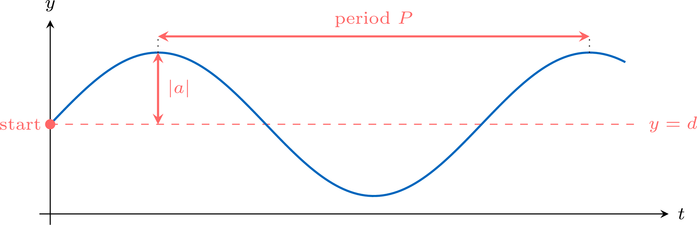
A quantity that repeats itself every $P$ units of time in a smooth wave, rising and falling symmetrically about a middle value, can be modelled by $y = a\sin(bt) + d$ or $y = a\cos(bt) + d$, where the angle $bt$ is measured in degrees.

Principal axis: $d = \dfrac{\text{maximum} + \text{minimum}}{2}$.
Amplitude: $|a| = \dfrac{\text{maximum} - \text{minimum}}{2}$.
Period: one period is one full turn of $360^\circ$, so $b = \dfrac{360}{P}$, in degrees per unit of time ($b > 0$).
Form and sign, read on the start of the data, at $t = 0$:
- on the principal axis and rising: $y = a\sin(bt) + d$ with $a > 0$;
- on the principal axis and falling: $y = a\sin(bt) + d$ with $a < 0$;
- at a maximum: $y = a\cos(bt) + d$ with $a > 0$;
- at a minimum: $y = a\cos(bt) + d$ with $a < 0$.
The time origin is chosen so that the data start at one of these four positions; data that start anywhere else need a horizontal translation of the curve.
Check the model on a data point, and set the calculator to degree mode before using it.

Example

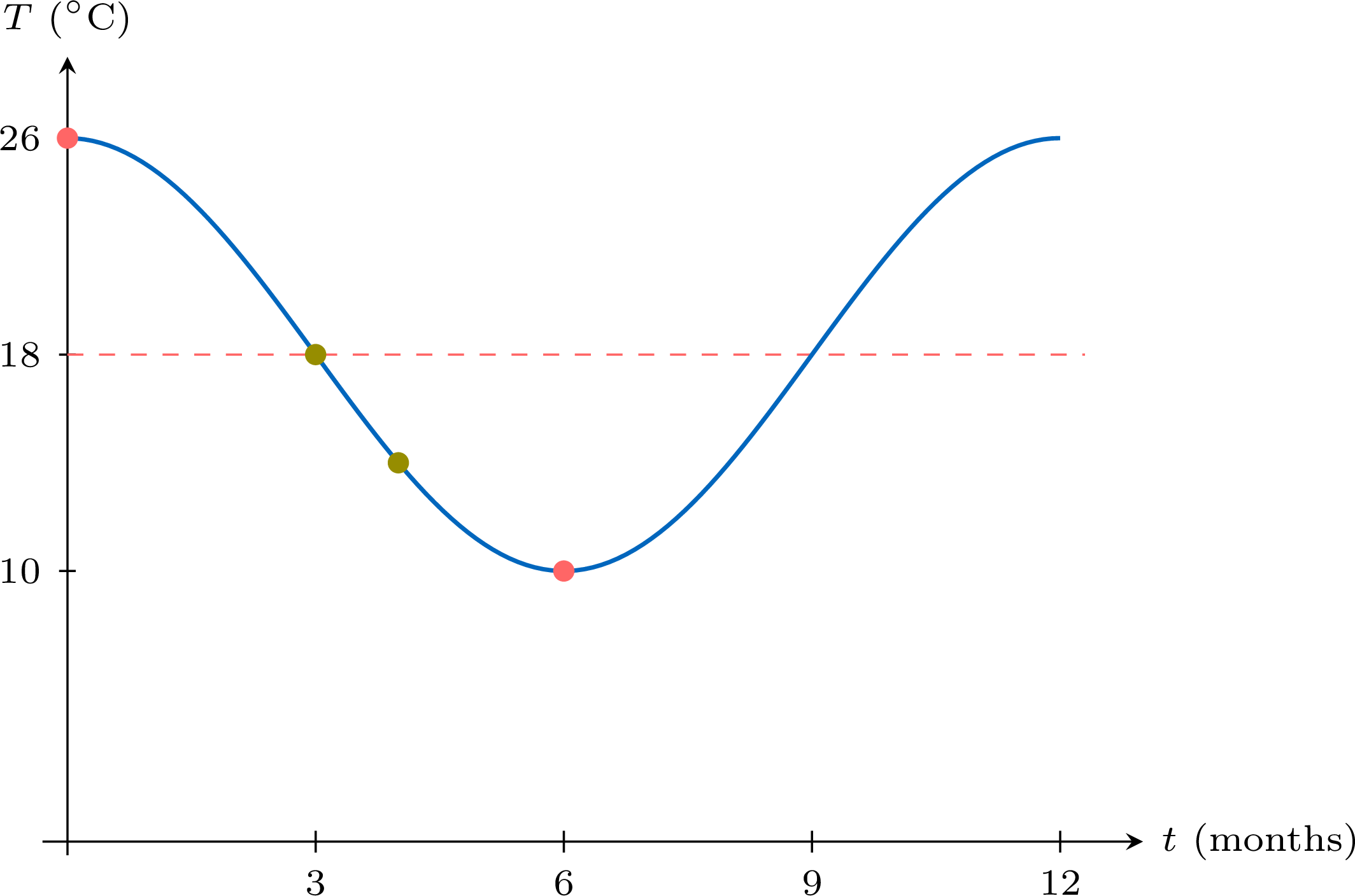
In a city of the southern hemisphere, the mean monthly temperature is highest in January, $26^\circ$C, and lowest in July, $10^\circ$C, and the pattern repeats every year. Let $t$ be the time in months, with $t = 0$ in January and $t = 6$ in July.

Find a model $T(t) = a\cos(bt) + d$ for the mean monthly temperature, the angle $bt$ being in degrees.
Use the model to estimate the mean temperature in April ($t = 3$) and in May ($t = 4$).

Answer

Following the Method:
- principal axis: $d = \dfrac{26 + 10}{2} = 18$;
- amplitude: $|a| = \dfrac{26 - 10}{2} = 8$;
- the period is $12$ months, so $b = \dfrac{360}{12} = 30$ (degrees per month);
- at $t = 0$ the temperature is at its maximum: the form $a\cos(bt) + d$ with $a > 0$, so $a = 8$.
The model is $T(t) = 8\cos(30t) + 18$. Check in July: $T(6) = 8\cos 180^\circ + 18 = -8 + 18 = 10$, the minimum of the data.
$$\begin{aligned}[t] T(3) &= 8\cos 90^\circ + 18 = 8 \times 0 + 18 = 18,\\ T(4) &= 8\cos 120^\circ + 18 = 8 \times \left(-\frac{1}{2}\right) + 18 = 14. \end{aligned}$$ The model estimates about $18^\circ$C in April and $14^\circ$C in May.

Skills to practice

Finding a Sinusoidal Model in Degrees

III Exam-Style Questions

Skills to practice

Working with Technology: Functions and Modelling
Working with Technology: Further Functions and Modelling

\(v\)	\(2\)	\(4\)	\(6\)	\(8\)
\(R\)	\(1.2\)	\(4.8\)	\(10.8\)	\(19.2\)

\(w\)	\(2\)	\(3\)	\(4\)	\(6\)
\(T\)	\(18\)	\(12\)	\(9\)	\(6\)

\(v\)	\(2\)	\(4\)	\(6\)	\(8\)
\(\frac{R}{v}\)	\(0.6\)	\(1.2\)	\(1.8\)	\(2.4\)
\(\frac{R}{v^2}\)	\(0.3\)	\(0.3\)	\(0.3\)	\(0.3\)