International Baccalaureate · DP 2: Analysis and Approaches HL
Continuous Random Variables and the Normal Distribution
I
Continuous Random Variables
I.1
Continuous Random Variables
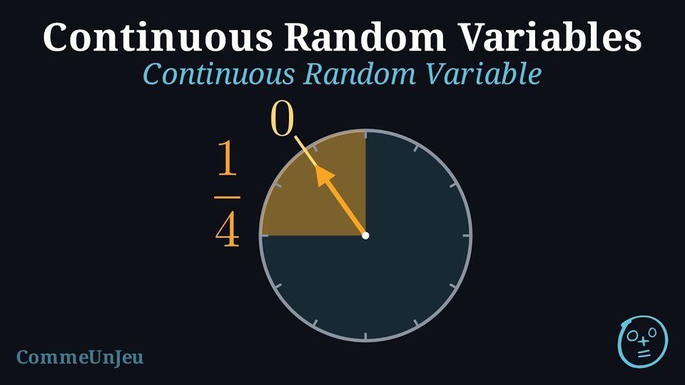
Consider a random experiment where a spinner is spun, and the continuous random variable \(X\) represents the angle spun, measured in degrees over the interval \([0, 360)\). 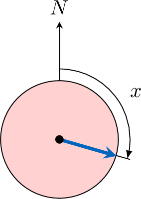
The probability that \(X\) assumes any precise value, such as \(x = 125.333\ldots\), is zero due to the infinite number of possible outcomes within a continuous range. However, we can calculate the probability that \(X\) lies within an interval, such as \([90, 180]\). We can think of this as summing the probabilities over tiny subintervals within this range:$$\begin{aligned}P(90 \leq X \leq 180) &= \sum_{x \in [90, 180]} P(x \leq X < x + \mathrm{d}x) \\
&= \sum_{x \in [90, 180]} \frac{P(x \leq X < x + \mathrm{d}x)}{dx} \cdot \mathrm{d}x\end{aligned}$$ Here, \(\mathrm{d}x\) represents an infinitesimally small interval, and the ratio, \(\frac{P(x \leq X < x + \mathrm{d}x)}{dx}\) is the probability per unit length. We define this as the probability density function, \(f(x)=\frac{P(x \leq X < x + \mathrm{d}x)}{dx}\). By the definition of integration, this summation becomes:$$P(90 \leq X \leq 180) = \int_{90}^{180} f(x) \, \mathrm{d}x$$ For a uniform spinner, the probability is evenly distributed across all angles, so the pdf is constant: \(f(x) = \frac{1}{360}\) for \(x \in [0, 360)\). Thus:$$\begin{aligned}P(90 \leq X \leq 180) &= \int_{90}^{180} \frac{1}{360} \, \mathrm{d}x \\
&= \left[ \frac{x}{360} \right]_{90}^{180} \\
&= \frac{180}{360} - \frac{90}{360} \\
&= \frac{1}{4}\end{aligned}$$ Hence, the probability of spinning an angle between 90 and 180 degrees is \(\frac{1}{4}\). 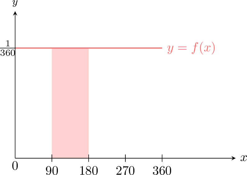
Definition — Continuous Random Variable
A random variable is continuous if its set of possible values is an entire interval of real numbers. A continuous random variable can take any value within its range, meaning there is an infinite number of possibilities. Skills to practice
- Distinguishing Discrete and Continuous Variables
I.2
Probability Density Functions
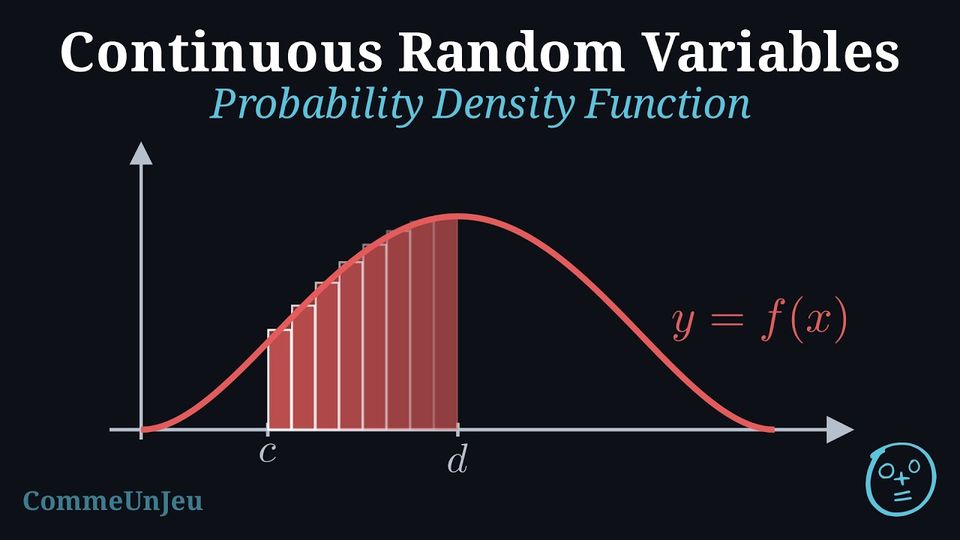
A probability density function describes the likelihood of a continuous random variable taking values within a specific range. Unlike discrete random variables, where probabilities are assigned to individual outcomes, continuous variables use the pdf to compute probabilities over intervals via integration.
Definition — Probability Density Function
A function \(f\) is a probability density function (pdf) on the interval \([a, b]\) if: - \(f(x) \geq 0\) for all \(x \in [a, b]\) (non-negative everywhere),
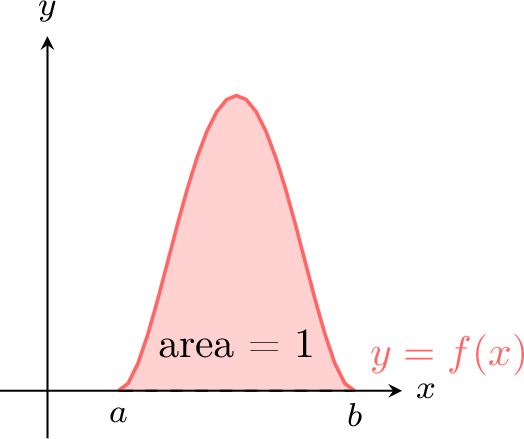
- \(\int_{a}^{b} f(x) \, \mathrm{d}x = 1\) (the total area under the curve equals 1).
Example
The random variable \(X\) takes values on \([0, 2]\) with density \(f(x) = \frac{x}{2}\). 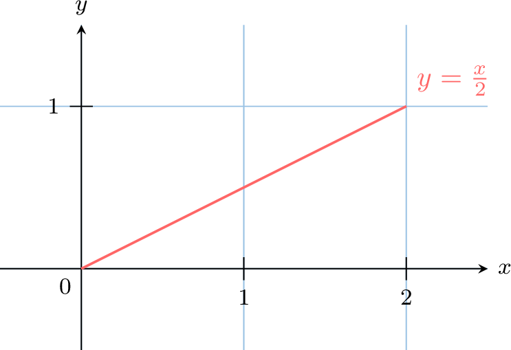
- \(f(x) = \frac{x}{2} \geq 0\) for all \(x \in [0,2]\), since \(x \geq 0\).
- Compute the total area: $$ \begin{aligned}[t] \int_{0}^{2} f(x) \, \mathrm{d}x &= \int_{0}^{2} \frac{x}{2} \, \mathrm{d}x \\ &= \left[ \frac{x^2}{4} \right]_{0}^{2} \\ &= \frac{2^2}{4} - 0 = 1 \end{aligned} $$ Since both conditions hold, \(f(x) = \frac{x}{2}\) is a valid pdf on \([0, 2]\).
Definition — Density of a Continuous Random Variable
A random variable \(X\) with values on \([a, b]\) has a density \(f\), if the probability that \(X\) lies between \(c\) and \(d\) (\(c, d \in [a, b]\) with \(c \leq d\)) is:$$P(c \leq X \leq d) = \int_{c}^{d} f(x) \, \mathrm{d}x$$ This represents the area under the curve \(y = f(x)\) from \(x = c\) to \(x = d\). 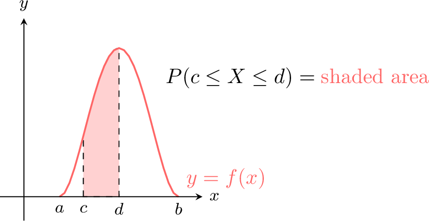
Remark
- Since \(f(x) \geq 0\), \(P(c \leq X \leq d) \geq 0\).
- Since \(\int_{a}^{b} f(x) \, \mathrm{d}x = 1\), \(P(a \leq X \leq b) = 1\).
A Given Value Has Probability Zero
Let \(X\) be a random variable with density \(f\) on an interval \(I\) and let \(c \in I\). The probability that \(X\) takes exactly the value \(c\) is the area of a segment of width zero: $$P(X = c) = \int_c^c f(x)\,\mathrm{d}x = 0.$$ The variable does take values, but no value announced in advance has a positive probability: among infinitely many possible values, each one weighs nothing. As a consequence, strict and non-strict inequalities give the same probabilities: \(P(c < X < d) = P(c \leq X \leq d)\), \(P(X < c) = P(X \leq c)\) and \(P(X > c) = P(X \geq c) = 1 - P(X \leq c)\).
An event of probability \(0\) is therefore not necessarily the empty event. For instance, a number is chosen at random in \([0, 1]\), the probability of landing in an interval \([c, d] \subseteq [0, 1]\) being its length \(d - c\): the sample space is \(U = [0, 1]\), an outcome \(\omega\) is the number chosen, and \(X(\omega) = \omega\) defines a random variable with density \(f(x) = 1\) on \([0, 1]\). The event \(\left(X = \frac{1}{2}\right)\) is the set \(\left\{\frac{1}{2}\right\}\): it is not empty, since the outcome \(\omega = \frac{1}{2}\) realises it, and yet \(P\left(X = \frac{1}{2}\right) = \int_{1/2}^{1/2} f(x)\,\mathrm{d}x = 0\). The impossible event \(\emptyset\) has probability \(0\), but the converse is false.
An event of probability \(0\) is therefore not necessarily the empty event. For instance, a number is chosen at random in \([0, 1]\), the probability of landing in an interval \([c, d] \subseteq [0, 1]\) being its length \(d - c\): the sample space is \(U = [0, 1]\), an outcome \(\omega\) is the number chosen, and \(X(\omega) = \omega\) defines a random variable with density \(f(x) = 1\) on \([0, 1]\). The event \(\left(X = \frac{1}{2}\right)\) is the set \(\left\{\frac{1}{2}\right\}\): it is not empty, since the outcome \(\omega = \frac{1}{2}\) realises it, and yet \(P\left(X = \frac{1}{2}\right) = \int_{1/2}^{1/2} f(x)\,\mathrm{d}x = 0\). The impossible event \(\emptyset\) has probability \(0\), but the converse is false.
Skills to practice
- Calculating Probabilities under the Curve
- Verifying a Probability Density Function
I.3
Expectation
From a Weighted Mean to an Integral
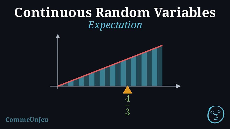
For a variable taking finitely many values \(x_1, \dots, x_n\), the expected value is the mean of the values weighted by their probabilities: \(E(X) = \sum x_i\,P(X = x_i)\). For a variable with density \(f\) on \([a ; b]\), cut \([a ; b]\) into small intervals of width \(h\). The probability of landing between \(x\) and \(x + h\) is close to the area of a rectangle, \(f(x) \times h\), so the weighted mean is close to the sum of the products \(x \times f(x) \times h\): a sum of rectangles, as in the rectangle method for the function \(x \mapsto x f(x)\). As \(h\) shrinks, this sum approaches the integral of that function, and the expected value becomes an integral: \(E(X) = \displaystyle\int_a^b x f(x)\,\mathrm{d}x\). In the same way, the variance \(\sum \left(x_i - E(X)\right)^2 P(X = x_i)\) becomes \(\displaystyle\int_a^b \left(x - E(X)\right)^2 f(x)\,\mathrm{d}x\).
Definition — Expectation
For a continuous random variable \(X\) with density \(f\) on \([a, b]\), the expected value is $$E(X) = \int_{a}^{b} x f(x) \, \mathrm{d}x.$$ 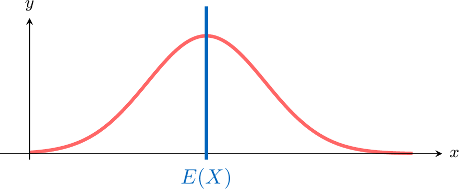
Example
The random variable \(X\) with values on \([0, 3]\) has density \(f(x) = \frac{x^2}{9}\): 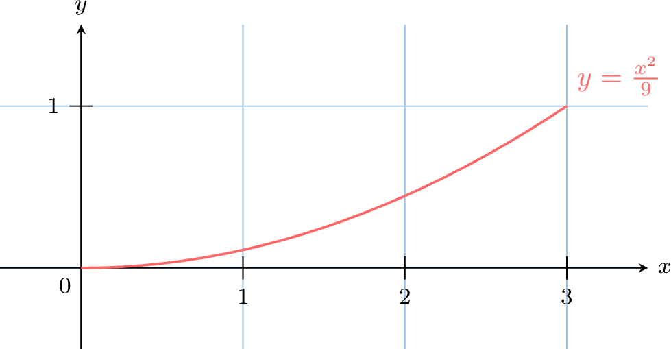
Compute \(E(X)\): $$ \begin{aligned}[t] E(X) &= \int_{0}^{3} x \cdot \frac{x^2}{9} \, \mathrm{d}x \\
&= \int_{0}^{3} \frac{x^3}{9} \, \mathrm{d}x \\
&= \left[ \frac{x^4}{36} \right]_{0}^{3} \\
&= \frac{3^4}{36} - 0 \\
&= 2.25 \end{aligned} $$ 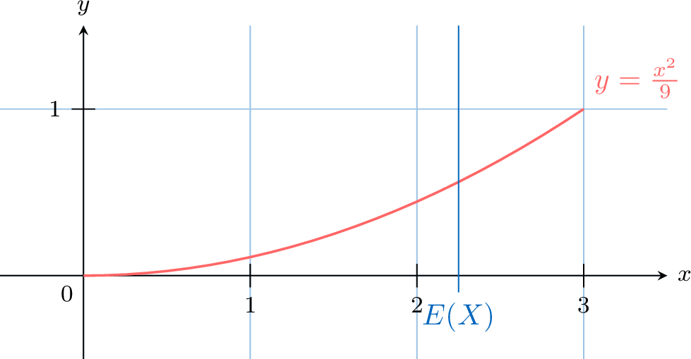
Skills to practice
- Calculating an Expectation
I.4
Variance and Standard Deviation
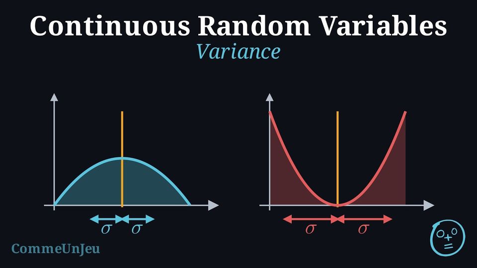
Definition — Variance and Standard Deviation
For a continuous random variable \(X\) with density \(f\) on \([a, b]\), the variance is$$V(X) = \int_{a}^{b} (x - E(X))^2 f(x) \, \mathrm{d}x.$$ The standard deviation is$$\sigma = \sqrt{V(X)}.$$ 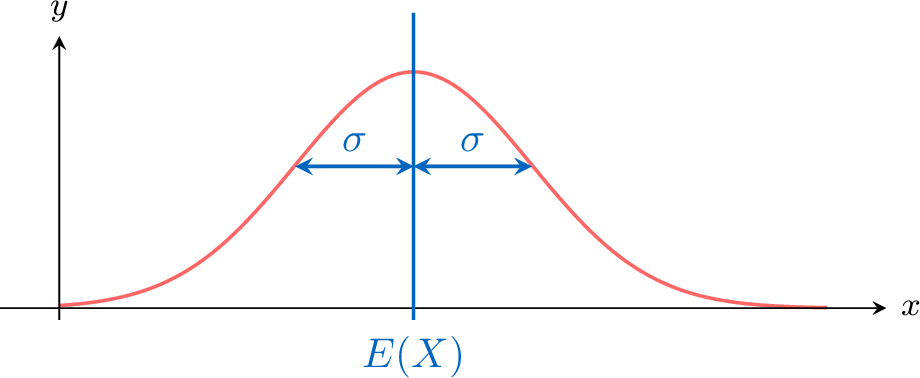
Proposition — Computing a Variance with an Integral
Let \(X\) have density \(f\) on \([a ; b]\), and let \(m = E(X)\). Then $$V(X) = \int_a^b x^2 f(x)\,\mathrm{d}x - m^2.$$ The integral \(\displaystyle\int_a^b x^2 f(x)\,\mathrm{d}x\) is written \(E(X^2)\): the formula reads \(V(X) = E(X^2) - [E(X)]^2\), as for a variable taking finitely many values.
For every \(x\) in \([a ; b]\), expanding the square gives \((x - m)^2 f(x) = x^2 f(x) - 2m\,x f(x) + m^2 f(x)\). Hence $$\begin{aligned} V(X) &= \int_a^b (x - m)^2 f(x)\,\mathrm{d}x && \text{(definition)}\\
&= \int_a^b x^2 f(x)\,\mathrm{d}x - 2m \int_a^b x f(x)\,\mathrm{d}x + m^2 \int_a^b f(x)\,\mathrm{d}x && \text{(linearity)}\\
&= \int_a^b x^2 f(x)\,\mathrm{d}x - 2m \times m + m^2 \times 1 && \text{(}E(X) = m\text{, total area } 1\text{)}\\
&= \int_a^b x^2 f(x)\,\mathrm{d}x - m^2. \end{aligned}$$
Example
The random variable \(X\) with values on \([0,2]\) has density \(f(x) = \frac{x}{2}\).Find \(V(X)\).
- Compute \(E(X)\): $$ \begin{aligned}[t] E(X) &= \int_{0}^{2} x \cdot \frac{x}{2} \, \mathrm{d}x \\ &= \int_{0}^{2} \frac{x^2}{2} \, \mathrm{d}x \\ &= \left[ \frac{x^3}{6} \right]_{0}^{2} \\ &= \frac{2^3}{6} - 0 \\ &= \frac{8}{6} \\ &= \frac{4}{3} \\ \end{aligned} $$
- Compute \(\int_{0}^{2} x^2 \cdot f(x) \, \mathrm{d}x\): $$ \begin{aligned}[t] \int_{0}^{2} x^2 \cdot f(x) \, \mathrm{d}x &=\int_{0}^{2} x^2 \cdot \frac{x}{2} \, \mathrm{d}x\\ &= \int_{0}^{2} \frac{x^3}{2} \, \mathrm{d}x \\ &= \left[ \frac{x^4}{8} \right]_{0}^{2} \\ &= \frac{2^4}{8} - 0 \\ &= \frac{16}{8} \\ &= 2 \end{aligned} $$
- Compute \(V(X)\) using the alternative formula: $$ \begin{aligned}[t] V(X) &= \int_{0}^{2} x^2 \cdot f(x) \, \mathrm{d}x - [E(X)]^2 \\ &= 2 - \left(\frac{4}{3}\right)^2 \\ &= 2 - \frac{16}{9} \\ &= \frac{18}{9} - \frac{16}{9} \\ &= \frac{2}{9} \end{aligned} $$
Skills to practice
- Calculating a Variance
I.5
Mode and Median
Definition — Mode and Median
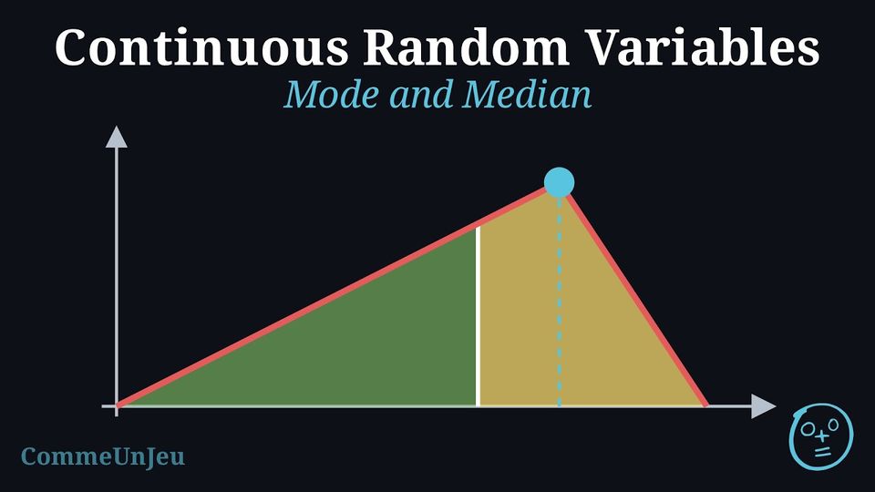
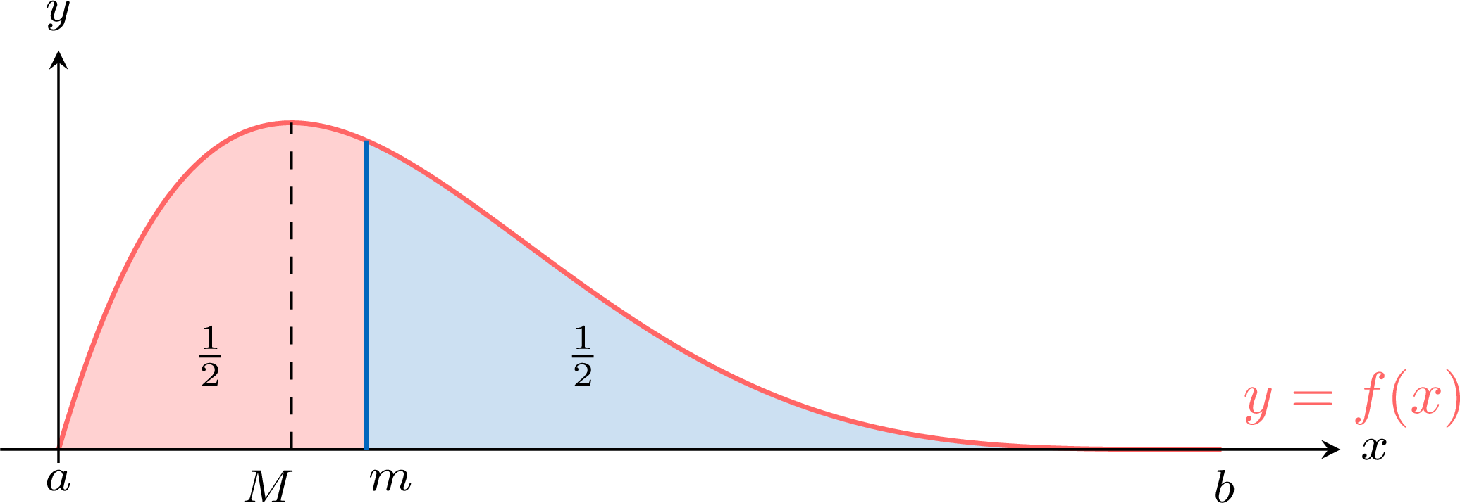
Let \(X\) be a continuous random variable with density \(f\) on \([a, b]\). - A mode of \(X\) is a value \(M\) of \([a, b]\) at which \(f\) reaches its greatest value: \(f(x) \leq f(M)\) for every \(x\) in \([a, b]\). The values of \(X\) are the most concentrated around a mode.
- The median of \(X\) is the number \(m\) of \([a, b]\) such that $$P(X \leq m) = \int_{a}^{m} f(x) \, \mathrm{d}x = \frac{1}{2}.$$ The vertical line \(x = m\) cuts the area under the curve into two halves: \(X\) is less than \(m\) with probability \(\frac{1}{2}\), and greater than \(m\) with probability \(\frac{1}{2}\). Such a number always exists, and it is unique when \(f(x) > 0\) for \(a < x < b\).
Method — Finding the Mode and the Median
For a continuous random variable \(X\) with density \(f\) on \([a, b]\): - Sketch the density: the sketch shows where \(f\) is greatest, and on which side of that point most of the area lies.
- Mode: find the greatest value of \(f\) on \([a, b]\). Inside the interval, a point where \(f'(x) = 0\) and \(f'\) changes from positive to negative is a local maximum. Compare the values of \(f\) there with its values at \(a\) and at \(b\) and, for a density defined piecewise, at the points where the pieces meet, where \(f'\) may not exist: the greatest value can be reached at any of these points. A density that increases on \([a, b]\) has its mode at \(b\); one that decreases, at \(a\).
- Median: solve \(\int_{a}^{m} f(x) \, \mathrm{d}x = \frac{1}{2}\) for \(m\), and keep the solution that lies in \([a, b]\). For a density defined piecewise, first compute the area under the first piece: if it is more than \(\frac{1}{2}\), the median lies in the first piece; if it is less than \(\frac{1}{2}\), in a later piece; if it equals \(\frac{1}{2}\), the median is the point where the first piece ends. When the equation cannot be solved by hand, solve it with the equation solver of a graphing calculator.
- Check: the area from \(a\) to \(m\) must be \(\frac{1}{2}\), and when the area on one side of the mode is more than \(\frac{1}{2}\), the median lies on that side. When the density is symmetric about a number \(c\), the median and the expectation are both equal to \(c\).
Example
Find the mode and the median of \(X\) in each case, then compare them with the expectation. - \(X\) has the density \(f(x) = \frac{x}{2}\) on \([0, 2]\), and its expectation is \(E(X) = \frac{4}{3}\).
- \(X\) has the density \(f(x) = 12x(1 - x)^2\) on \([0, 1]\), and its expectation is \(E(X) = \frac{2}{5}\). Give the median to \(3\) significant figures.
- The density \(f(x) = \frac{x}{2}\) increases on \([0, 2]\), so its greatest value is at the right end, \(f(2) = 1\): the mode is \(M = 2\).
The median \(m\) lies in \([0, 2]\) and satisfies $$\begin{aligned}[t] \int_{0}^{m} \frac{x}{2} \, \mathrm{d}x &= \frac{1}{2} && \text{(definition of the median)}\\ \left[\frac{x^2}{4}\right]_{0}^{m} &= \frac{1}{2}\\ \frac{m^2}{4} &= \frac{1}{2}\\ m^2 &= 2. \end{aligned}$$ Of the two solutions \(\sqrt{2}\) and \(-\sqrt{2}\), only \(\sqrt{2}\) lies in \([0, 2]\): \(m = \sqrt{2} \approx 1.41\).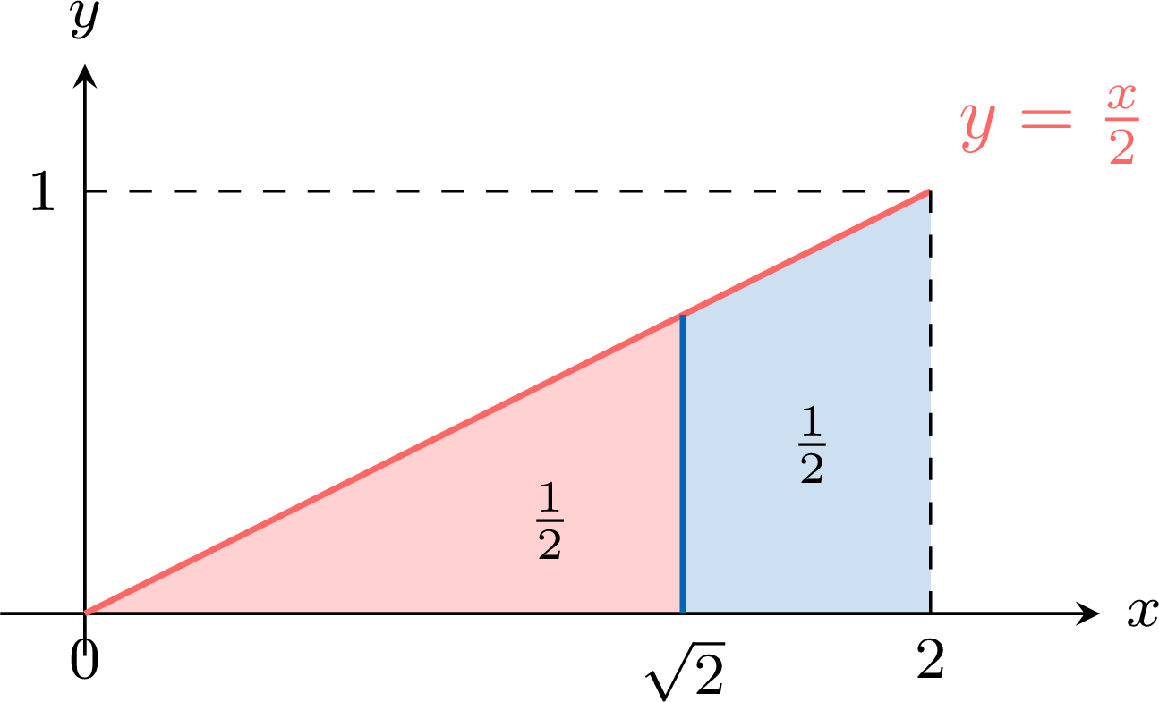
- The mode is where \(f\) is greatest. By the product rule, $$\begin{aligned}[t] f'(x) &= 12(1 - x)^2 + 12x \times 2(1 - x) \times (-1) && \text{(product rule)}\\
&= 12(1 - x)\big[(1 - x) - 2x\big]\\
&= 12(1 - x)(1 - 3x). \end{aligned}$$ On \([0, 1]\), the factor \(1 - x\) is positive except at \(1\), so \(f'(x)\) has the sign of \(1 - 3x\): positive for \(x < \frac{1}{3}\), negative for \(\frac{1}{3} < x < 1\). The function \(f\) increases, then decreases: its greatest value is \(f\left(\frac{1}{3}\right) = 12 \times \frac{1}{3} \times \frac{4}{9} = \frac{16}{9}\), greater than \(f(0) = f(1) = 0\). The mode is \(M = \frac{1}{3}\).
The median \(m\) satisfies, after expanding \(12x(1 - x)^2 = 12x - 24x^2 + 12x^3\), $$\begin{aligned}[t] \int_{0}^{m} \left(12x - 24x^2 + 12x^3\right) \mathrm{d}x &= \frac{1}{2} && \text{(definition of the median)}\\ \Big[6x^2 - 8x^3 + 3x^4\Big]_{0}^{m} &= \frac{1}{2}\\ 6m^2 - 8m^3 + 3m^4 &= \frac{1}{2}. \end{aligned}$$ This equation of degree \(4\) is solved with the equation solver on \([0, 1]\): \(m = 0.3857275\ldots\), so \(m \approx 0.386\). Check: \(6m^2 - 8m^3 + 3m^4 = 0.5000\) with this value.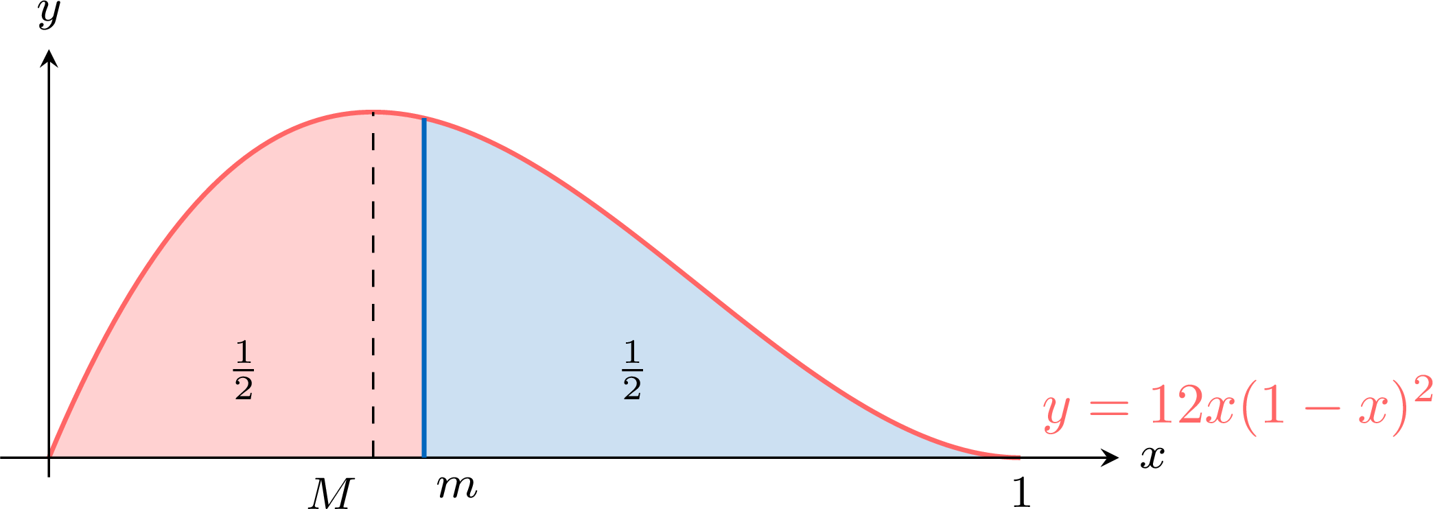
Example
The time \(X\), in hours, that a courier takes to deliver a parcel has the density $$f(x) = \begin{cases} \dfrac{x}{6} & \text{if } 0 \leq x \leq 3, \\
\dfrac{4 - x}{2} & \text{if } 3 < x \leq 4. \end{cases}$$ - Sketch the density and find the mode of \(X\).
- Find the median of \(X\).
- The expectation of \(X\) is \(E(X) = \frac{7}{3}\). Place the mode, the median and the expectation in increasing order, and explain the order with the shape of the density.
- The first piece increases from \(f(0) = 0\) to \(f(3) = \frac{3}{6} = \frac{1}{2}\); the second decreases from \(\frac{4 - 3}{2} = \frac{1}{2}\) at \(3\) to \(f(4) = 0\). The two pieces meet at \(x = 3\), where \(f\) reaches its greatest value \(\frac{1}{2}\): the mode is \(M = 3\) hours.
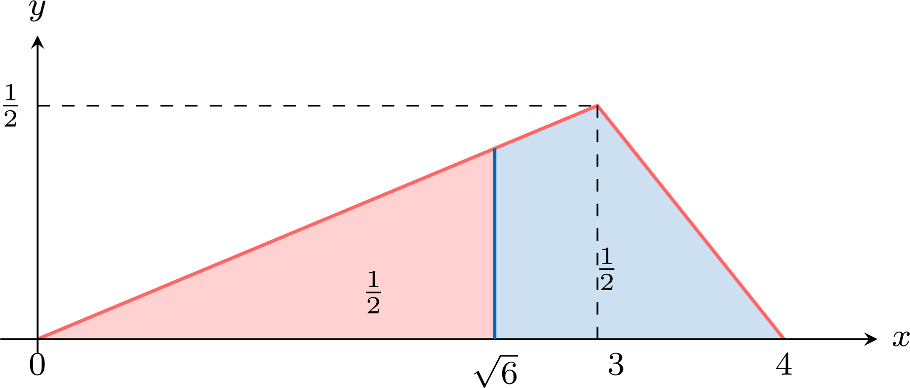
- The area under the first piece is $$\int_{0}^{3} \frac{x}{6} \, \mathrm{d}x = \left[\frac{x^2}{12}\right]_{0}^{3} = \frac{9}{12} = \frac{3}{4},$$ more than \(\frac{1}{2}\): the median lies in \([0, 3]\), where \(f(x) = \frac{x}{6}\). It satisfies $$\begin{aligned}[t] \int_{0}^{m} \frac{x}{6} \, \mathrm{d}x &= \frac{1}{2} && \text{(definition of the median)}\\ \frac{m^2}{12} &= \frac{1}{2}\\ m^2 &= 6, \end{aligned}$$ and \(m = \sqrt{6} \approx 2.45\) hours, the solution that lies in \([0, 3]\).
- The three numbers are \(E(X) = \frac{7}{3} \approx 2.33 < m = \sqrt{6} \approx 2.45 < M = 3\). The density rises slowly from \(0\) to \(3\) and falls quickly from \(3\) to \(4\): its long tail is on the left, towards the short times, and it pulls the median, and the expectation further still, below the mode.
Skills to practice
- Recognising the Mode and the Median
- Finding the Mode and the Median
I.6
The Continuous Uniform Distribution
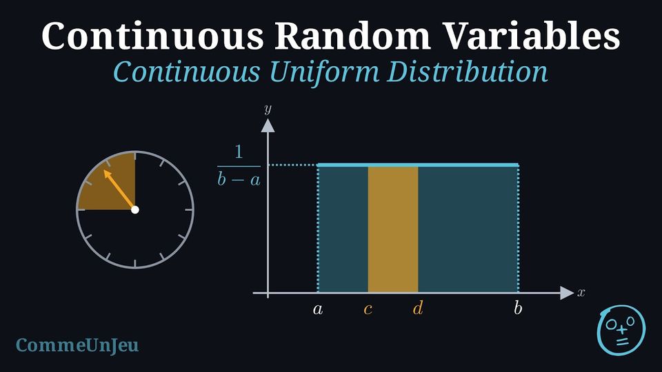
The continuous uniform distribution applies to events that are equally likely across an interval, such as the spinner example. The density is constant over the range.
Definition — Continuous Uniform Distribution
Let \(a\) and \(b\) be real numbers with \(a < b\). A continuous random variable \(X\) follows a continuous uniform distribution on \([a, b]\) if its density is:$$f(x) = \frac{1}{b - a} \quad \text{for} \quad a \leq x \leq b$$ 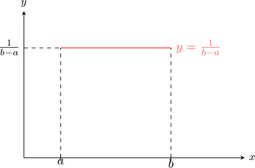
Proposition — Properties
Let \( X \) be a continuous random variable following a continuous uniform distribution on \([a, b]\): - for all \(c, d \in [a, b]\) with \(c \leq d\): \(P(c \leq X \leq d) = \frac{d - c}{b - a}\),
- \(E(X) = \frac{a + b}{2}\).
- \(V(X) = \frac{(b-a)^2}{12}\).
- Probability: $$ \begin{aligned}[t] P(c \leq X \leq d) &= \int_{c}^{d} \frac{1}{b - a} \, \mathrm{d}x \\ &= \left[ \frac{x}{b - a} \right]_{c}^{d} \\ &= \frac{d - c}{b - a} \end{aligned} $$
- Expected value: $$ \begin{aligned}[t] E(X) &= \int_{a}^{b} x \cdot \frac{1}{b - a} \, \mathrm{d}x \\ &= \left[ \frac{x^2}{2(b - a)} \right]_{a}^{b} \\ &= \frac{b^2 - a^2}{2(b - a)}\\ &= \frac{(b - a)(b + a)}{2(b - a)}\\ &= \frac{a + b}{2} \end{aligned} $$
- Variance: We use the formula \(V(X) = E(X^2) - [E(X)]^2\). First, we compute \(E(X^2)\). $$ \begin{aligned}[t] E(X^2) &= \int_{a}^{b} x^2 \cdot \frac{1}{b-a} \, \mathrm{d}x \\ &= \frac{1}{b-a} \left[ \frac{x^3}{3} \right]_{a}^{b} \\ &= \frac{b^3-a^3}{3(b-a)} = \frac{(b-a)(b^2+ab+a^2)}{3(b-a)} = \frac{a^2+ab+b^2}{3} \end{aligned} $$ Now we can compute the variance: $$ \begin{aligned}[t] V(X) &= \frac{a^2+ab+b^2}{3} - \left(\frac{a+b}{2}\right)^2 \\ &= \frac{4(a^2+ab+b^2) - 3(a+b)^2}{12} \\ &= \frac{4a^2+4ab+4b^2 - 3(a^2+2ab+b^2)}{12} \\ &= \frac{4a^2+4ab+4b^2 - 3a^2-6ab-3b^2}{12} \\ &= \frac{a^2-2ab+b^2}{12} = \frac{(b-a)^2}{12} \end{aligned} $$
Skills to practice
- Testing Knowledge of the Continuous Uniform Distribution
II
The Normal Distribution
II.1
Normal Curves and Probabilities
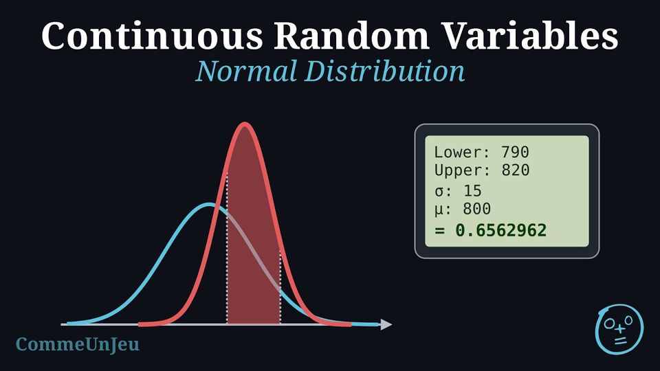
The normal distribution is a key continuous distribution in statistics, often used to model real-world phenomena (e.g., heights, test scores) due to the Central Limit Theorem. This theorem states that the sum or average of many independent random variables, under certain conditions, approximates a normal distribution as the sample size increases. The normal curve is bell-shaped, symmetric, and centred at its mean.
For example, we plot a histogram of the heights of boys at the university. The distribution represented by the histogram follows a bell-shaped curve, also known as a normal distribution. 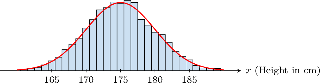
For example, we plot a histogram of the heights of boys at the university. The distribution represented by the histogram follows a bell-shaped curve, also known as a normal distribution.
Definition — Normal Distribution
A continuous random variable \(X\) follows a normal distribution if its density is:$$f(x) = \frac{1}{\sigma \sqrt{2\pi}} e^{-\frac{1}{2} \left( \frac{x - \mu}{\sigma} \right)^2}, \quad -\infty < x < \infty$$ where \(\mu\) is the mean and \(\sigma^2\) is the variance. The graph is a normal curve (bell-shaped), denoted \(X \sim \mathcal{N}(\mu, \sigma^2)\). 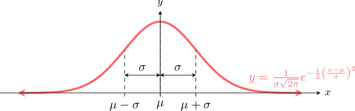
Proposition — Expectation and Variance
For \(X \sim \mathcal{N}(\mu, \sigma^2)\): - \(E(X) = \mu\),
- \(V(X) = \sigma^2\).
Method — Calculating a Normal Probability with Technology
For \(X \sim \mathcal{N}(\mu, \sigma^2)\), the probability of an interval is an area under the normal curve, an integral of the density whose antiderivative cannot be written with the usual functions (polynomials, exponentials, logarithms): the normal cumulative distribution function of a graphing calculator computes it. Its name depends on the model: Normal C.D, normalcdf, normCdf. - State the model: \(X \sim \mathcal{N}(\mu, \sigma^2)\), with its mean \(\mu\) and its standard deviation \(\sigma\) — not the variance \(\sigma^2\): for \(X \sim \mathcal{N}(50, 16)\), \(\sigma = 4\).
- Sketch and shade first: draw a bell curve centred at \(\mu\), mark the bound or bounds, and shade the region of the event. The sketch predicts the size of the answer: a region that contains the mean and most of the curve has a probability close to \(1\), a region that lies on one side of \(\mu\) a probability less than \(0.5\), and a region far in one tail a probability close to \(0\).
- Enter the bounds of the region, as in the table below, then \(\mu\) and \(\sigma\), each in the field that carries its name: the order of the fields depends on the model, and the command
normalcdftakes the lower bound, the upper bound, \(\mu\), then \(\sigma\). A region with no left end takes as its lower bound a negative number so large that it lies very many standard deviations below the mean, such as \(-10^{99}\), and a region with no right end a positive number as large, such as \(10^{99}\), as its upper bound. - Compare the screen with the sketch, and report the probability to \(3\) significant figures, unless the question asks otherwise.
| Event | Lower bound | Upper bound |
| \(a < X < b\) | \(a\) | \(b\) |
| \(X < b\) | \(-10^{99}\) | \(b\) |
| \(X > a\) | \(a\) | \(10^{99}\) |
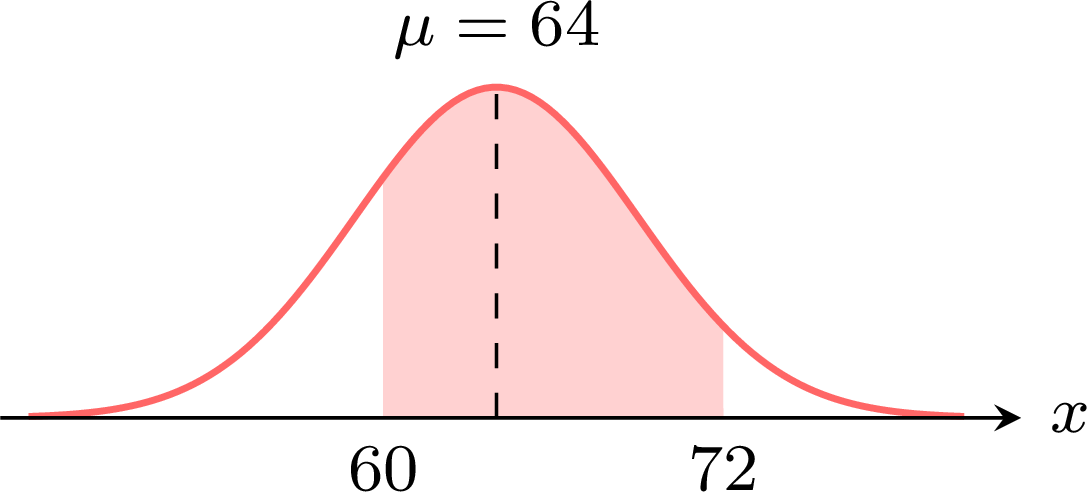
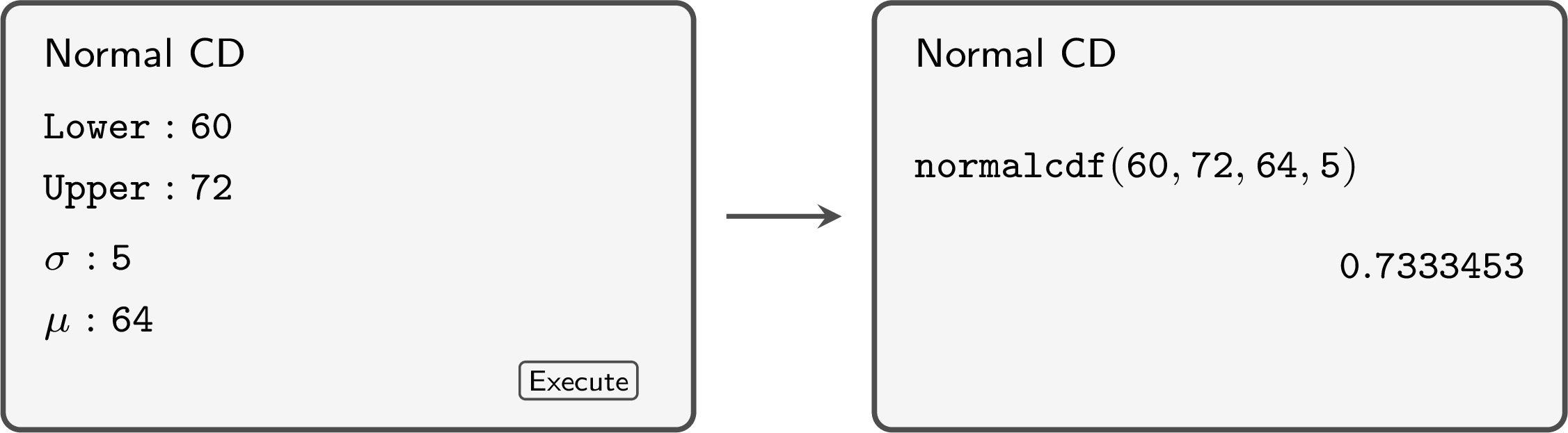
The sketch and the mock-up show the computation of \(P(60 < X < 72)\) for \(X \sim \mathcal{N}(64, 5^2)\): the region contains the mean and most of the curve, and the screen gives \(P(60 < X < 72) \approx 0.733\).
Example
A bakery sells loaves whose mass \(X\), in grams, is normally distributed with mean \(800\) g and standard deviation \(15\) g. Find the probability that a loaf chosen at random has a mass: - between \(790\) g and \(820\) g;
- less than \(780\) g;
- more than \(822\) g.
The model is \(X \sim \mathcal{N}(800, 15^2)\): \(\mu = 800\) and \(\sigma = 15\). The three regions are sketched and shaded first. 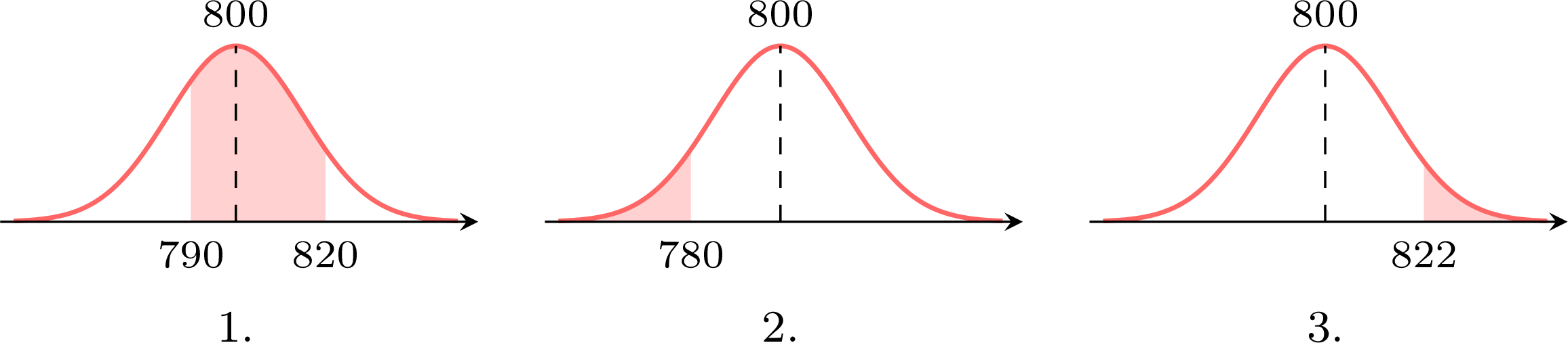
- The region contains the mean and more than half of the curve. With lower bound \(790\), upper bound \(820\), \(\sigma = 15\) and \(\mu = 800\), the screen gives \(0.6562962\): $$P(790 < X < 820) \approx 0.656.$$
- The region is the left tail below \(780\), a small part of the curve. With lower bound \(-10^{99}\) and upper bound \(780\), the screen gives \(0.0912112\): $$P(X < 780) \approx 0.0912.$$
- The region is the right tail above \(822\). With lower bound \(822\) and upper bound \(10^{99}\), the screen gives \(0.0712334\): $$P(X > 822) \approx 0.0712.$$
Example
The battery life \(X\) of a model of phone, in hours, is normally distributed with mean \(14.5\) h and standard deviation \(1.8\) h. - Find \(P(X \geq 12)\).
- A shop sells \(400\) of these phones. Find the expected number of phones whose battery lasts less than \(12\) hours.
- Without technology, find \(P(X \leq 14.5)\).
The model is \(X \sim \mathcal{N}(14.5, 1.8^2)\). 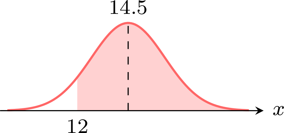
- The region lies to the right of \(12\), which is below the mean: it contains the mean and more than half of the curve, so the probability is greater than \(0.5\). With lower bound \(12\), upper bound \(10^{99}\), \(\sigma = 1.8\) and \(\mu = 14.5\), the screen gives \(0.9175667\): $$P(X \geq 12) \approx 0.918.$$
- A battery lasts less than \(12\) hours with the probability of the complementary event, the unshaded left tail: $$\begin{aligned}[t] P(X < 12) &= 1 - P(X \geq 12) && \text{(complementary event)}\\ &= 1 - 0.9175667\ldots\\ &= 0.0824333\ldots \end{aligned}$$ Each of the \(400\) phones has this probability, so the expected number is $$400 \times P(X < 12) = 400 \times 0.0824333\ldots \approx 32.97.$$ About \(33\) phones are expected to last less than \(12\) hours.
- The normal curve is symmetric about its mean \(\mu = 14.5\), so the area to the left of the mean is half of the total area: $$P(X \leq 14.5) = 0.5.$$
Skills to practice
- Reading and Entering a Normal Model
- Finding Probabilities with Technology
II.2
The Empirical Rule
Proposition — Empirical Rule for Normal Distribution
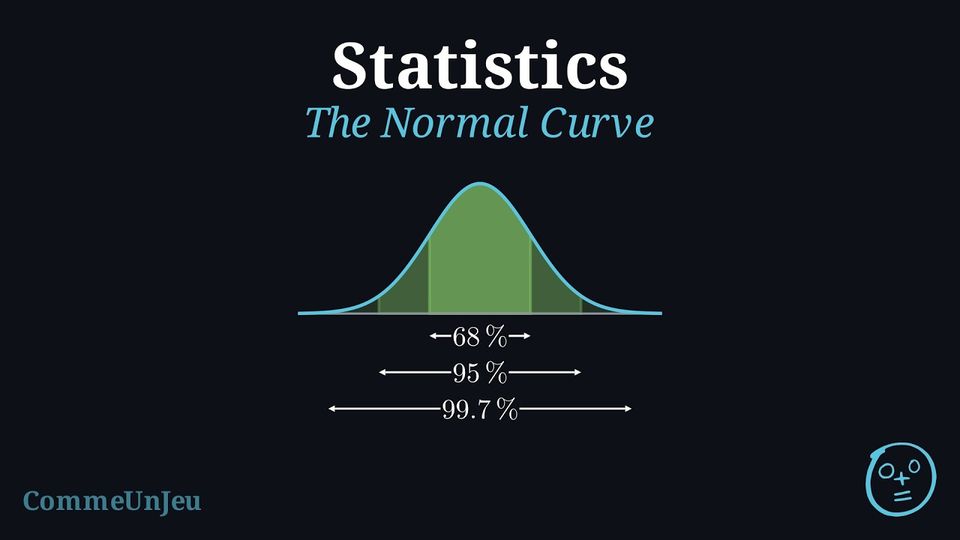
For \(X \sim \mathcal{N}(\mu, \sigma^2)\), the probabilities for intervals centred at the mean are approximately: - \(P(\mu - \sigma \leq X \leq \mu + \sigma) \approx 68.3\pourcent\)
- \(P(\mu - 2\sigma \leq X \leq \mu + 2\sigma) \approx 95.4\pourcent\)
- \(P(\mu - 3\sigma \leq X \leq \mu + 3\sigma) \approx 99.7\pourcent\)
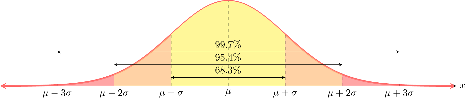
The Empirical Rule states that for a normal distribution, specific percentages of data lie within intervals around the mean. Due to the symmetry of the normal curve, we can break these down to find the probabilities for individual sections, each one standard deviation wide. For example, by symmetry, the area from \(\mu\) to \(\mu+\sigma\) is half of the total area from \(\mu-\sigma\) to \(\mu+\sigma\): $$P(\mu \leq X \leq \mu + \sigma) = \frac{P(\mu - \sigma \leq X \leq \mu + \sigma)}{2} \approx 34.13\pourcent$$ This gives us a detailed map of the normal distribution: 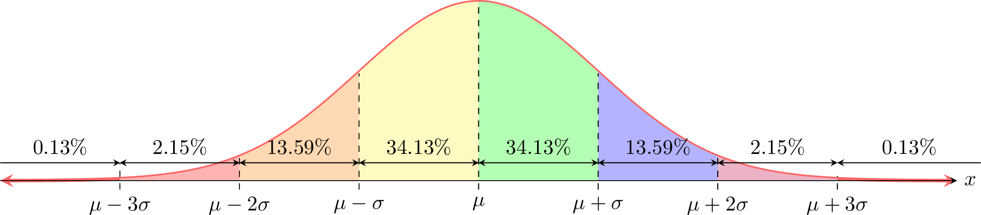
Example
Students’ heights at a school are normally distributed with mean \(\mu = 172 \, \text{cm}\) and standard deviation \(\sigma = 8 \, \text{cm}\). - Find the percentage of students with heights between 164 cm and 172 cm.
- Find the percentage between 164 cm and 180 cm.
- Find the percentage with heights above 196 cm.
- Find the percentage with heights below 196 cm.
- In a group of 500 students, how many are expected to have heights between 164 cm and 180 cm?
First, we label the distribution with the given mean and standard deviation: 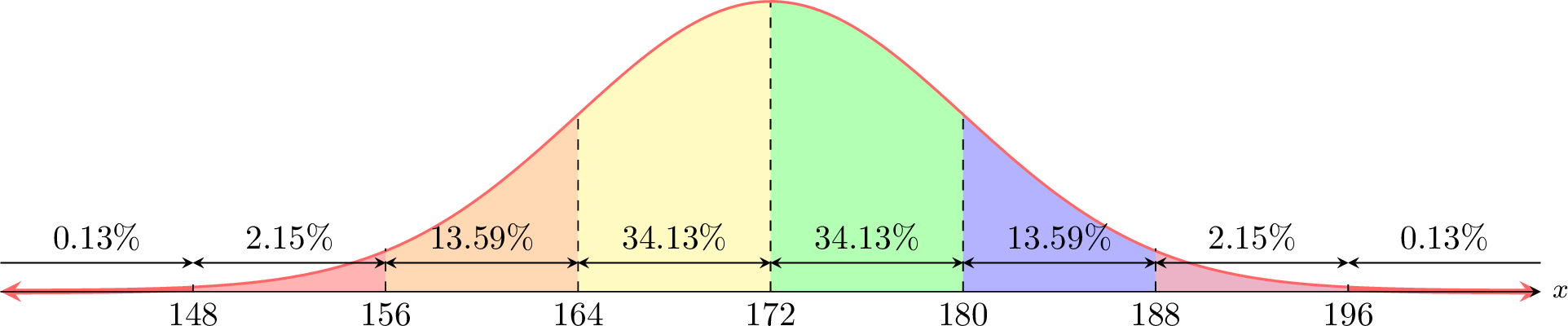
- \(P(164 \leq X \leq 172) = P(\mu - \sigma \leq X \leq \mu) = 34.13\pourcent\).
- \(P(164 \leq X \leq 180) = P(\mu - \sigma \leq X \leq \mu + \sigma) = 34.13\pourcent + 34.13\pourcent = 68.26\pourcent\).
- \(P(X > 196) = P(X \geq \mu + 3\sigma) = 0.13\pourcent\).
- \(P(X < 196) = 1 - P(X \geq 196) = 100\pourcent - 0.13\pourcent = 99.87\pourcent\).
- Expected number = \(68.26\pourcent \times 500 = 0.6826 \times 500 \approx 341\) students.
Skills to practice
- Using the Empirical Rule
II.3
Quantiles and the Inverse Normal
Definition — Quantile
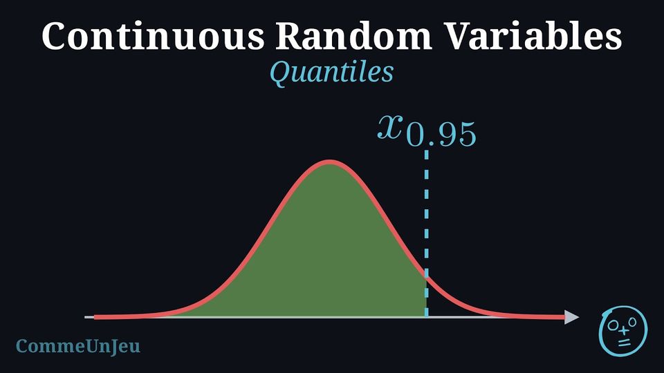
The \(p\)-quantile of a random variable \(X\) is the value \(x_p\) such that \(P(X \leq x_p) = p\). For example, the \(0.95\)-quantile (or 95th percentile) is the value \(x_{0.95}\) below which 95\(\pourcent\) of the distribution's values lie. Method — Finding a Value with the Inverse Normal Function
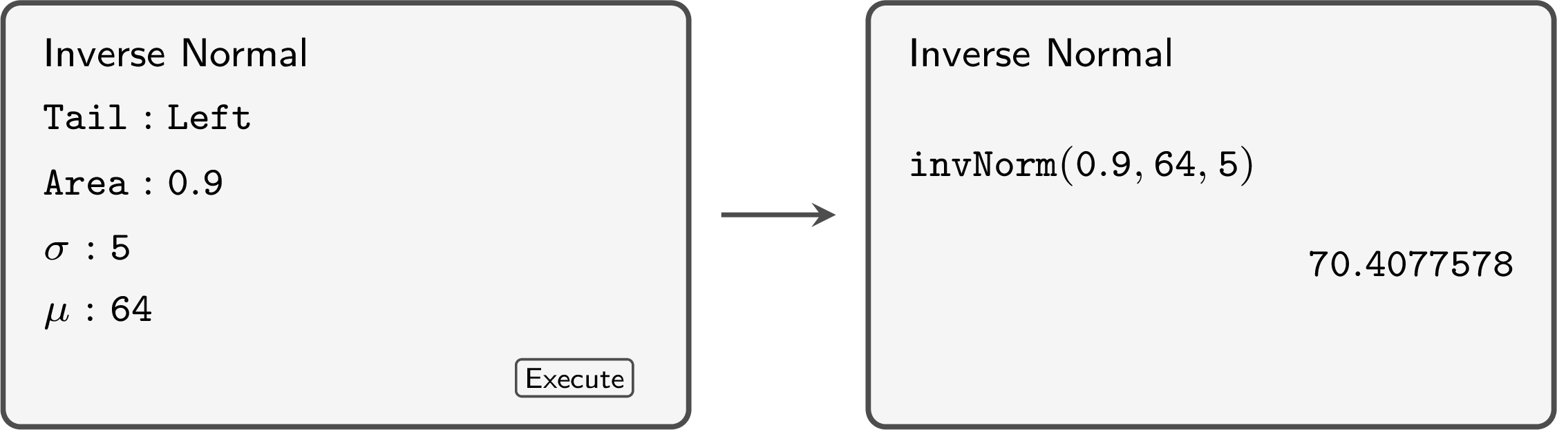
The reverse question gives a probability and asks for a value of \(X\). The inverse normal function of the calculator (Inverse Normal, invNorm) returns the value \(k\) such that \(P(X < k) = p\), for \(0 < p < 1\), from the area \(p\) to the left of \(k\), \(\sigma\) and \(\mu\). - State the model \(X \sim \mathcal{N}(\mu, \sigma^2)\) and name the unknown value \(k\).
- Sketch and shade: place \(k\) on the side of \(\mu\) that the probability indicates — a left area less than \(0.5\) puts \(k\) below the mean — and shade the given area.
- Turn the condition into a left area. The condition \(P(X < k) = p\) is entered as it is; \(P(X > k) = q\) becomes \(P(X < k) = 1 - q\). An interval centred on \(\mu\) that contains the proportion \(p\) of the values leaves \(\frac{1 - p}{2}\) in each tail: its ends are the values with left areas \(\frac{1 - p}{2}\) and \(\frac{1 + p}{2}\).
- Enter the area, \(\mu\) and \(\sigma\), each in its field (the command
invNormtakes the area, \(\mu\), then \(\sigma\); the tail is set to the left, on the models that ask for one), then check the position of \(k\) against the sketch and report it to \(3\) significant figures, or to the precision of the data.
Example
The scores \(X\) on an entrance test are normally distributed with mean \(500\) and standard deviation \(80\). - A scholarship is offered to the top \(12\pourcent\) of the candidates. Find the minimum score for a scholarship.
- The lowest \(5\pourcent\) of the candidates are offered extra support. Find the score below which a candidate is offered support.
The model is \(X \sim \mathcal{N}(500, 80^2)\). 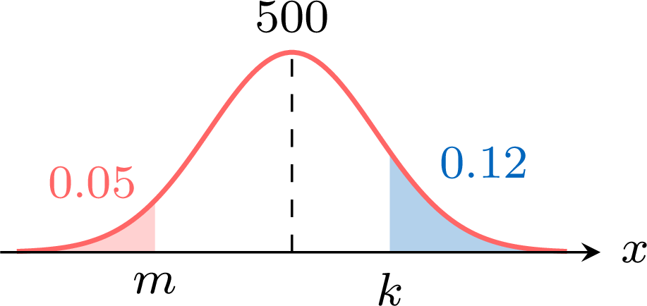
- Let \(k\) be the minimum score: \(P(X > k) = 0.12\). The right tail is small, so \(k\) lies above the mean. As a left area, $$\begin{aligned}[t] P(X < k) &= 1 - P(X > k) && \text{(complementary event)}\\ &= 1 - 0.12\\ &= 0.88. \end{aligned}$$ The inverse normal function with area \(0.88\), \(\sigma = 80\) and \(\mu = 500\) gives \(593.9989\ldots\): the minimum score for a scholarship is about \(594\).
- Let \(m\) be the score: \(P(X < m) = 0.05\), a left tail, so \(m\) lies below the mean. The inverse normal function with area \(0.05\), \(\sigma = 80\) and \(\mu = 500\) gives \(368.4117\ldots\): a candidate who scores below about \(368\) is offered support.
Example
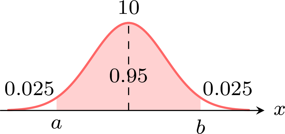
A machine makes bolts whose diameter \(X\), in millimetres, is normally distributed with mean \(10.00\) mm and standard deviation \(0.04\) mm. - Find the interval, centred on the mean, that contains the diameters of \(95\pourcent\) of the bolts. Give its ends to \(3\) decimal places.
- A bolt is rejected when its diameter is less than \(9.93\) mm or more than \(10.07\) mm. Find the proportion of bolts rejected.
The model is \(X \sim \mathcal{N}(10, 0.04^2)\).
- The central \(95\pourcent\) leaves \(\frac{1 - 0.95}{2} = 0.025\) in each tail. Its ends \(a\) and \(b\) therefore have the left areas \(0.025\) and \(0.975\):
- A bolt is accepted when \(9.93 \leq X \leq 10.07\). With lower bound \(9.93\), upper bound \(10.07\), \(\sigma = 0.04\) and \(\mu = 10\), the normal cumulative distribution function gives \(0.9198817\), so $$\begin{aligned}[t] P(\text{rejected}) &= 1 - P(9.93 \leq X \leq 10.07) && \text{(complementary event)}\\ &= 1 - 0.9198817\ldots\\ &\approx 0.0801. \end{aligned}$$ About \(8.01\pourcent\) of the bolts are rejected. This agrees with question 1: the interval of accepted diameters is narrower than the central interval that holds \(95\pourcent\) of the bolts, so more than \(5\pourcent\) fall outside it.
Skills to practice
- Finding a Value with the Inverse Normal Function
- Setting a Threshold with Percentiles
III
Standard Scores and Standardising
III.1
Standard Scores
Definition — Variance and Standard Deviation
The variance \(V\) of a data set measures the average of the squared distances of the values from the mean \(\bar{x}\). When the values \(x_i\) have frequencies \(n_i\) (with \(N = \sum n_i\)): $$ V = \frac{1}{N}\sum_{i=1}^{k} n_i (x_i - \bar{x})^2 . $$ The standard deviation \(\sigma\) is the square root of the variance: $$ \sigma = \sqrt{V} = \sqrt{\frac{1}{N}\sum_{i=1}^{k} n_i (x_i - \bar{x})^2} . $$ The variance is expressed in the squared unit of the data, whereas the standard deviation is back in the original unit, which makes it the natural measure of typical distance to the mean. This is the population (descriptive) variance, with denominator \(N\). Definition — Standard Score
The standard score (or \(z\)-score) of an observation \(x\) in a data set whose mean is \(\bar{x}\) and whose standard deviation is \(\sigma > 0\) is: $$ z = \frac{x - \bar{x}}{\sigma} . $$ It rescales the raw value \(x\) by measuring its distance to the mean of its data set, counted in standard deviations.
The standard score states how many standard deviations the observation \(x\) lies from the mean of its data set, and in which direction: \(z>0\) means \(x\) is above the mean, \(z<0\) means below, and the magnitude of \(z\) measures how far. Because \(z\) has no unit, it lets you fairly compare observations coming from different data sets measured on different scales: the larger standard score marks the relatively stronger position within its own set (when a higher raw value indicates a better result).
Example
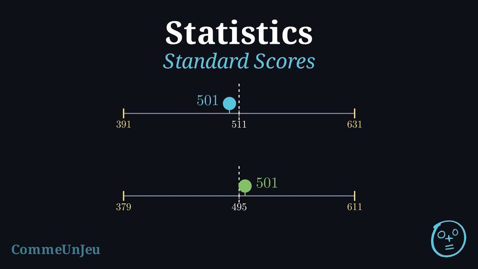
A student sits two tests measured on different scales. On the Mathematics test, the class scores have mean \(\bar{x} = 511\) and standard deviation \(\sigma = 120\). On the Reading test, the class scores have mean \(\bar{x} = 495\) and standard deviation \(\sigma = 116\). The student scores \(501\) on both tests. On which test did the student perform better, relative to the class?
The two raw scores are equal (\(501\)), but each belongs to a different data set, so they are compared through their standard scores. $$ \begin{aligned} z_{\text{Maths}} &= \frac{x - \bar{x}}{\sigma} &&\text{(standard score)} \\
&= \frac{501 - 511}{120} &&\text{(Maths data set)} \\
&\approx -0.083 ; &&\text{(below the mean)} \\
z_{\text{Read}} &= \frac{501 - 495}{116} &&\text{(Reading data set)} \\
&\approx 0.052 . &&\text{(above the mean)} \end{aligned} $$ Although the raw scores are identical, \(z_{\text{Read}} \approx 0.052 > z_{\text{Maths}} \approx -0.083\). The student stands above the mean in Reading but below it in Mathematics, so the student performed better on the Reading test relative to the class.
Skills to practice
- Converting Between Values and Standard Scores
III.2
The Standard Normal Distribution
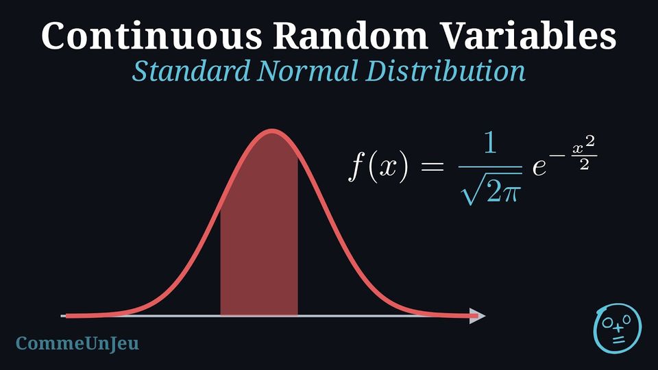
Definition — Standard Normal Distribution
A continuous random variable \(X\) follows a standard normal distribution if it has a mean of 0 and a variance of 1. Its density is:$$f(x) = \frac{1}{\sqrt{2\pi}} e^{-\frac{x^2}{2}}, \quad -\infty < x < \infty$$ This is denoted \(X \sim \mathcal{N}(0, 1)\). 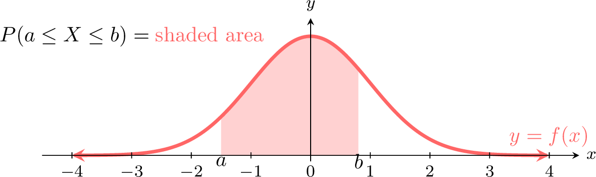
Remark
The total probability is 1:$$\int_{-\infty}^{\infty} \frac{1}{\sqrt{2\pi}} e^{-\frac{x^2}{2}} \, \mathrm{d}x = 1$$ This is the area under the entire curve. 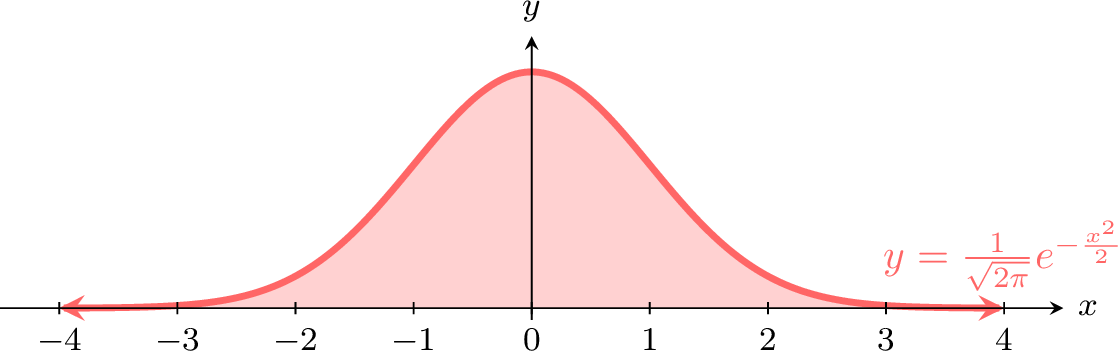
Skills to practice
- Reading Areas under the Standard Normal Curve
III.3
Standardising a Normal Variable
Proposition — Standardising a Normal Variable
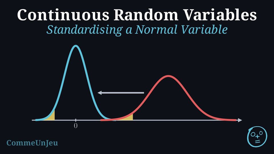
If \(X \sim \mathcal{N}(\mu, \sigma^2)\), then the standardised variable $$Z = \frac{X - \mu}{\sigma}$$ follows the standard normal distribution: \(Z \sim \mathcal{N}(0, 1)\). Consequently, for every real number \(x\), $$P(X \leq x) = P(Z \leq z) \qquad \text{where} \qquad z = \frac{x - \mu}{\sigma},$$ and, for \(x_1 < x_2\) with standardised values \(z_1\) and \(z_2\), \(P(x_1 \leq X \leq x_2) = P(z_1 \leq Z \leq z_2)\).The number \(z\) is the standardised value (or \(z\)-value) of \(x\): the number of standard deviations between \(x\) and the mean, positive when \(x > \mu\) and negative when \(x < \mu\).
Let \(z\) be a real number. Since \(\sigma > 0\), the inequality \(\frac{X - \mu}{\sigma} \leq z\) is equivalent to \(X \leq \mu + \sigma z\). With the density of \(X\) and the substitution \(t = \frac{x - \mu}{\sigma}\), for which \(\mathrm{d}x = \sigma\,\mathrm{d}t\), the bound \(x = \mu + \sigma z\) becomes \(t = z\) and \(x \to -\infty\) becomes \(t \to -\infty\): $$\begin{aligned}[t] P(Z \leq z) &= P(X \leq \mu + \sigma z) && \text{(multiply by } \sigma > 0 \text{, add } \mu)\\
&= \int_{-\infty}^{\mu + \sigma z} \frac{1}{\sigma\sqrt{2\pi}}\, e^{-\frac{1}{2}\left(\frac{x - \mu}{\sigma}\right)^2} \,\mathrm{d}x && \text{(density of } X)\\
&= \int_{-\infty}^{z} \frac{1}{\sigma\sqrt{2\pi}}\, e^{-\frac{t^2}{2}}\, \sigma \,\mathrm{d}t && \text{(substitution)}\\
&= \int_{-\infty}^{z} \frac{1}{\sqrt{2\pi}}\, e^{-\frac{t^2}{2}} \,\mathrm{d}t. \end{aligned}$$ Hence, for \(a < b\), \(P(a < Z \leq b) = P(Z \leq b) - P(Z \leq a) = \int_{a}^{b} \frac{1}{\sqrt{2\pi}}\, e^{-\frac{t^2}{2}} \,\mathrm{d}t\): the probabilities of \(Z\) are the areas under the density of the standard normal distribution, so \(Z \sim \mathcal{N}(0, 1)\).
Finally, for every real number \(x\), the inequality \(X \leq x\) is equivalent to \(\frac{X - \mu}{\sigma} \leq \frac{x - \mu}{\sigma}\), that is to \(Z \leq z\), so \(P(X \leq x) = P(Z \leq z)\); the probability of an interval follows by difference.
Finally, for every real number \(x\), the inequality \(X \leq x\) is equivalent to \(\frac{X - \mu}{\sigma} \leq \frac{x - \mu}{\sigma}\), that is to \(Z \leq z\), so \(P(X \leq x) = P(Z \leq z)\); the probability of an interval follows by difference.
Standardising explains why the empirical rule holds for every normal distribution: for every \(k > 0\), $$P(\mu - k\sigma \leq X \leq \mu + k\sigma) = P(-k \leq Z \leq k),$$ a probability that depends neither on \(\mu\) nor on \(\sigma\). With \(k = 1\), \(2\) and \(3\), the standard normal distribution gives \(68.3\pourcent\), \(95.4\pourcent\) and \(99.7\pourcent\), whatever the mean and the standard deviation. The standardised value plays for a normal variable the part that the standard score plays for an observation in a data set: it counts the standard deviations from the mean, and it lets values of different normal variables be compared. Standardising also brings every normal variable back to the single distribution \(\mathcal{N}(0, 1)\), whose parameters are known: this is what makes an unknown mean or standard deviation reachable.
Method — Finding an Unknown Mean or Standard Deviation
When \(\mu\) or \(\sigma\) is unknown, the inverse normal function cannot be used on \(X\), since it needs both parameters. Standardising moves the condition to \(Z \sim \mathcal{N}(0, 1)\), whose parameters are known. - Write each condition as a left area: \(P(X < x) = p\), where a condition \(P(X > x) = q\) becomes \(P(X < x) = 1 - q\).
- Sketch: place \(x\) on the side of \(\mu\) that \(p\) indicates; a left area less than \(0.5\) puts \(x\) below the mean, so its standardised value is negative.
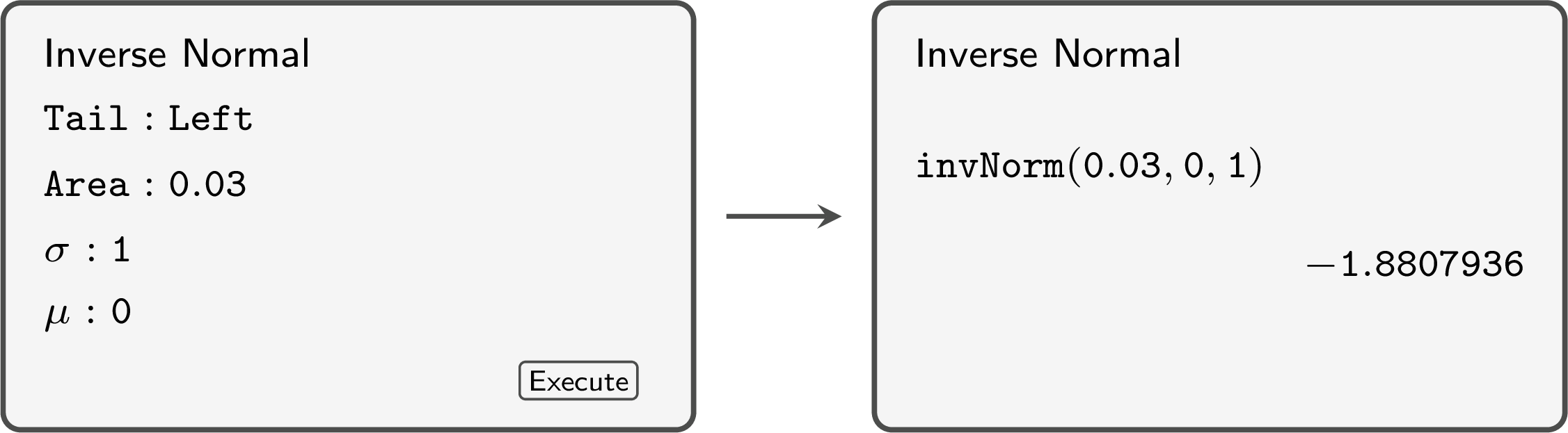
- Standardise and read \(z\): \(P(X < x) = P\left(Z < \frac{x - \mu}{\sigma}\right) = p\), so \(\frac{x - \mu}{\sigma} = z\), where \(z\) is given by the inverse normal function with area \(p\), \(\sigma = 1\) and \(\mu = 0\).
- Solve for the unknown, from \(x - \mu = z\sigma\):
- \(\sigma\) known: \(\mu = x - z\sigma\);
- \(\mu\) known: \(\sigma = \frac{x - \mu}{z}\), which requires \(z \neq 0\). A condition at the median (\(p = 0.5\), so \(z = 0\)) only says that \(x = \mu\) and gives no information on \(\sigma\);
- both unknown: two conditions with different values of \(z\) give the system \(\mu + z_1\sigma = x_1\) and \(\mu + z_2\sigma = x_2\); subtracting the equations gives \(\sigma = \frac{x_2 - x_1}{z_2 - z_1}\), then \(\mu = x_1 - z_1\sigma\).
- Keep \(z\) unrounded in the calculator's memory, round \(\mu\) and \(\sigma\) only at the end, and check: \(\sigma\) must be positive, and the normal cumulative distribution function with the values found must give back the probabilities of the question.
Example
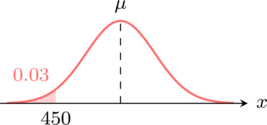
A machine fills jars of honey. The mass \(X\) of honey in a jar, in grams, is normally distributed with standard deviation \(4\) g. - \(3\pourcent\) of the jars contain less than \(450\) g. Find the mean mass \(\mu\), to \(1\) decimal place.
- The machine is set to the mean \(\mu = 456\) g, and a maintenance can reduce the standard deviation. Find the standard deviation \(\sigma\) for which only \(1\pourcent\) of the jars contain less than \(450\) g, to \(3\) significant figures.
- The model is \(X \sim \mathcal{N}(\mu, 4^2)\) with \(\mu\) unknown, and \(P(X < 450) = 0.03\): a small left area, so \(450\) lies below the mean.
- Now \(\mu = 456\) is known and \(\sigma\) is unknown: \(P(X < 450) = 0.01\), so \(\frac{450 - 456}{\sigma} = z\), where the inverse normal function with area \(0.01\), \(\sigma = 1\) and \(\mu = 0\) gives \(z = -2.3263479\ldots\), which is not zero. Then $$\begin{aligned}[t] \frac{450 - 456}{\sigma} &= z && \text{(standardised value of 450)}\\ \sigma &= \frac{450 - 456}{z}\\ &= \frac{-6}{-2.3263479\ldots}\\ &= 2.5791\ldots \end{aligned}$$ The standard deviation must be reduced to \(\sigma \approx 2.58\) g. It is positive, as it must be: \(450 - 456\) and \(z\) are both negative, since \(450\) lies below the mean.
Example
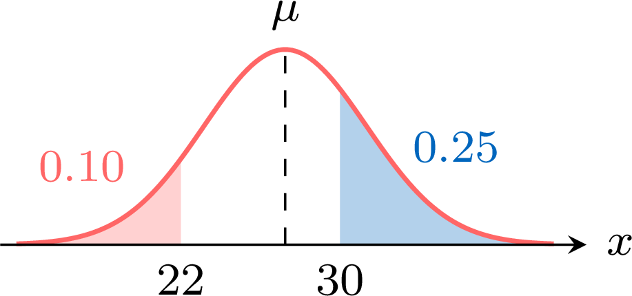
In a running club, the time \(X\) that a member takes to run \(5\) km, in minutes, is normally distributed. \(10\pourcent\) of the members run it in less than \(22\) minutes, and \(25\pourcent\) of them take more than \(30\) minutes. - Find the mean \(\mu\) and the standard deviation \(\sigma\) of \(X\), to \(3\) significant figures.
- Find the proportion of the members who run \(5\) km in less than \(25\) minutes.
- Both parameters are unknown, and the two conditions are written as left areas: \(P(X < 22) = 0.10\) and \(P(X < 30) = 1 - 0.25 = 0.75\). The first puts \(22\) below the mean, the second \(30\) above it.
- With the unrounded values stored, lower bound \(-10^{99}\), upper bound \(25\), the normal cumulative distribution function gives \(P(X < 25) = 0.2918\ldots\): about \(29.2\pourcent\) of the members run \(5\) km in less than \(25\) minutes. With \(\mu\) and \(\sigma\) rounded to \(27.2\) and \(4.09\) first, the same calculation gives \(0.2953\ldots\), which already changes the third significant figure: this is why the values are rounded only at the end.
Skills to practice
- Reading a Standardised Value
- Finding an Unknown Mean or Standard Deviation
- Finding the Mean and the Standard Deviation from Two Conditions
IV
Combining Models
IV.1
Counting Successes Defined by a Normal Model
Method — Counting Successes Defined by a Normal Model
A measurement often decides whether an item is a success: a loaf is underweight when its mass is less than a given value, an athlete qualifies when a jump is longer than a given length. Counting such items among \(n\) combines two models. - One item: compute the probability of success \(p\) with the normal model, for example \(p = P(X > a)\) with the normal cumulative distribution function, and keep \(p\) unrounded in the memory of the calculator.
- Several items: when the measurements of the \(n\) items all follow this normal model and are independent, each item is a success with the same probability \(p\), independently of the others, so the number \(Y\) of successes follows the binomial distribution \(\mathcal{B}(n, p)\).
- Compute with the binomial model: \(P(Y = k) = \binom{n}{k}p^k(1 - p)^{n - k}\); for “at least one”, the complementary event gives \(P(Y \geq 1) = 1 - (1 - p)^n\); the binomial functions of the calculator give the other events.
- Round only at the end: a rounded value of \(p\), raised to a power, changes the last significant figures of the answer.
Example
The mass \(X\), in grams, of the eggs of a farm is normally distributed with mean \(62\) g and standard deviation \(4\) g. An egg is sold as large when its mass is more than \(67\) g. A box holds \(6\) eggs chosen at random, whose masses are independent. - Find the probability that an egg is large.
- Find the probability that a box holds exactly \(2\) large eggs.
- Find the probability that a box holds at least one large egg.
- The model of one mass is \(X \sim \mathcal{N}(62, 4^2)\), and an egg is large when \(X > 67\), a right tail. With lower bound \(67\), upper bound \(10^{99}\), \(\sigma = 4\) and \(\mu = 62\), the normal cumulative distribution function gives \(p = P(X > 67) = 0.1056497\ldots\), so \(p \approx 0.106\).
- Let \(Y\) be the number of large eggs in a box. The masses of the \(6\) eggs all follow the model of question 1 and are independent, so each egg is large with the same probability \(p\), independently of the others: \(Y \sim \mathcal{B}(6, p)\) with \(p = 0.1056497\ldots\) kept in memory. Then $$\begin{aligned}[t] P(Y = 2) &= \binom{6}{2}p^2(1 - p)^4 && \text{(binomial distribution)}\\ &= 15 \times 0.1056497\ldots^2 \times 0.8943502\ldots^4\\ &\approx 0.107. \end{aligned}$$
- The event “at least one large egg” is the complement of “no large egg”: $$\begin{aligned}[t] P(Y \geq 1) &= 1 - P(Y = 0) && \text{(complementary event)}\\ &= 1 - (1 - p)^6\\ &= 1 - 0.8943502\ldots^6\\ &\approx 0.488. \end{aligned}$$ With \(p\) rounded to \(0.106\) before the power, the same computation gives \(1 - 0.894^6 \approx 0.489\): the third significant figure changes, which is why \(p\) is rounded only at the end.
Skills to practice
- Counting Successes with a Binomial Model
V
Going further
Skills to practice
- Solving Problems without Technology
- Solving Problems with Technology
- Quiz
Jump to section