International Baccalaureate · DP 1: Analysis and Approaches HL
Transformations of Functions
I
Translations, Stretches and Reflections
I.1
Translations
Recappreviously studied — click to reread
Function transformations take a basic “parent” function and modify it to create a new, related function. A sequence of transformations can translate, stretch or reflect the graph of the parent function.
Understanding these transformations makes it possible to predict the graph of a more complicated function from a simpler one, and to model real-world phenomena by adjusting a basic function to fit observed data. The transformations are vertical and horizontal translations, stretches (a stretch with a scale factor between \(0\) and \(1\) is also called a compression) and reflections.
Understanding these transformations makes it possible to predict the graph of a more complicated function from a simpler one, and to model real-world phenomena by adjusting a basic function to fit observed data. The transformations are vertical and horizontal translations, stretches (a stretch with a scale factor between \(0\) and \(1\) is also called a compression) and reflections.
Definition — Vertical Translation by Adding a Constant
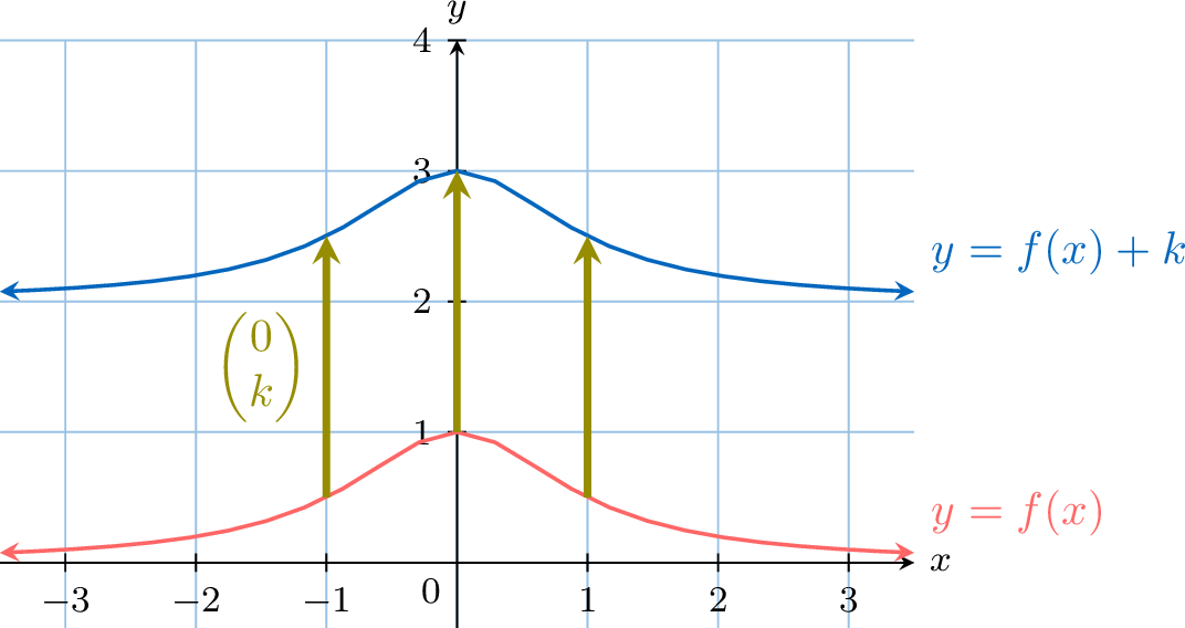
A vertical translation shifts the graph of a function up or down. The transformation is defined by:$$g(x) = f(x) + k$$ This transformation maps a point \((x, y)\) on the graph of \(f\) to a new point \((x, y+k)\) on the graph of \(g\). - If \(k>0\), the graph is translated \(\boldsymbol{k}\) units up.
- If \(k<0\), the graph is translated \(\boldsymbol{|k|}\) units down.
Definition — Horizontal Translation
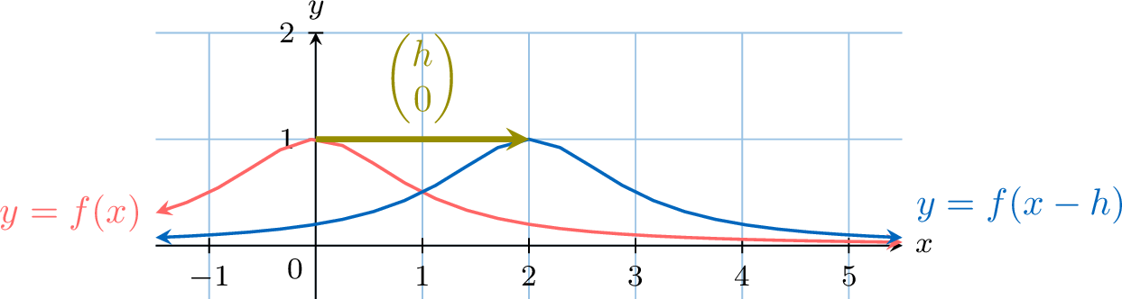
A horizontal translation shifts the graph of a function left or right. The transformation is defined by:$$g(x) = f(x-h)$$ This transformation maps a point \((x, y)\) on the graph of \(f\) to a new point \((x+h, y)\) on the graph of \(g\). - If \(h>0\), the graph is translated \(\boldsymbol{h}\) units to the right.
- If \(h<0\), the graph is translated \(\boldsymbol{|h|}\) units to the left.
Example
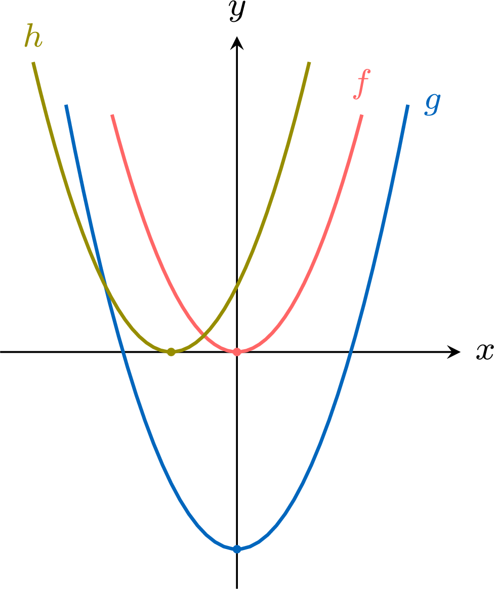
From the graph of \(f(x) = x^2\), plot \(g(x) = f(x) - 3\) and \(h(x) = f(x + 1)\). - \(g(x) = f(x) - 3\): every output is lowered by \(3\) — a vertical translation \(3\) units down. The vertex \((0, 0)\) moves to \((0, -3)\).
- \(h(x) = f(x + 1)\): the input \(x = -1\) now plays the role \(0\) used to play — a horizontal translation \(1\) unit to the left. The vertex \((0, 0)\) moves to \((-1, 0)\).
Translation by a Vector
The vertical and the horizontal translations combine into one. The translation by the vector \(\begin{pmatrix} h \\ k \end{pmatrix}\) moves each point \((x, y)\) of the graph of \(f\) to the point \((X, Y) = (x + h, y + k)\). Since \(x = X - h\) and \(Y = f(x) + k\), the image points satisfy \(Y = f(X - h) + k\); writing \((x, y)\) again for the coordinates, the image of the graph of \(y = f(x)\) is the graph of $$y = f(x - h) + k.$$ For example, the translation by the vector \(\begin{pmatrix} 3 \\ -2 \end{pmatrix}\) maps the graph of \(y = x^2\) onto the graph of \(y = (x - 3)^2 - 2\), and its vertex \((0, 0)\) to \((3, -2)\).
Skills to practice
- Translating Graphs
I.2
Stretches
Recappreviously studied — click to reread
Definition — Vertical Stretch
A vertical stretch stretches or compresses the graph of a function vertically. It is defined, for a number \(a \neq 0\), by:$$g(x) = a \cdot f(x)$$ This transformation maps a point \((x, y)\) to \((x, ay)\). - If \(|a|>1\), the graph is stretched vertically by a factor of \(|a|\).
- If \(0 < |a| < 1\), the graph is compressed vertically by a factor of \(|a|\).
- If \(a < 0\), the stretch or compression is followed by a reflection in the \(x\)-axis (\(a = -1\) gives the reflection alone).

Definition — Horizontal Stretch
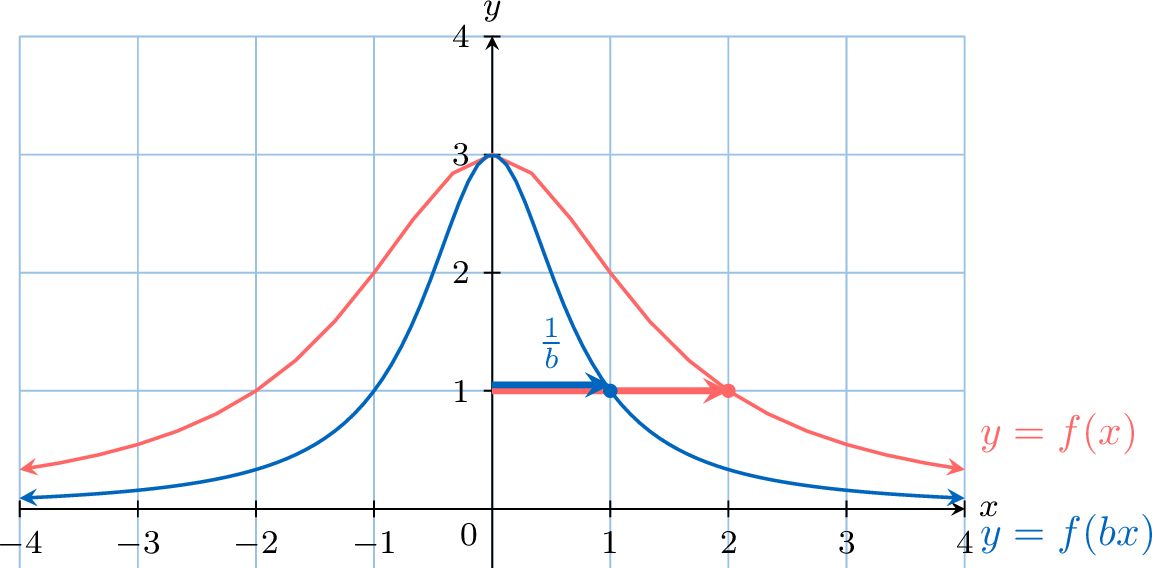
A horizontal stretch stretches or compresses the graph of a function horizontally. It is defined, for a number \(b \neq 0\), by:$$g(x) = f(bx)$$ This transformation maps a point \((x, y)\) to a new point \((\frac{x}{b}, y)\). - If \(|b|>1\), the graph is compressed horizontally by a factor of \(\frac{1}{|b|}\).
- If \(0 < |b| < 1\), the graph is stretched horizontally by a factor of \(\frac{1}{|b|}\).
- If \(b < 0\), the stretch or compression is followed by a reflection in the \(y\)-axis (\(b = -1\) gives the reflection alone).
Example
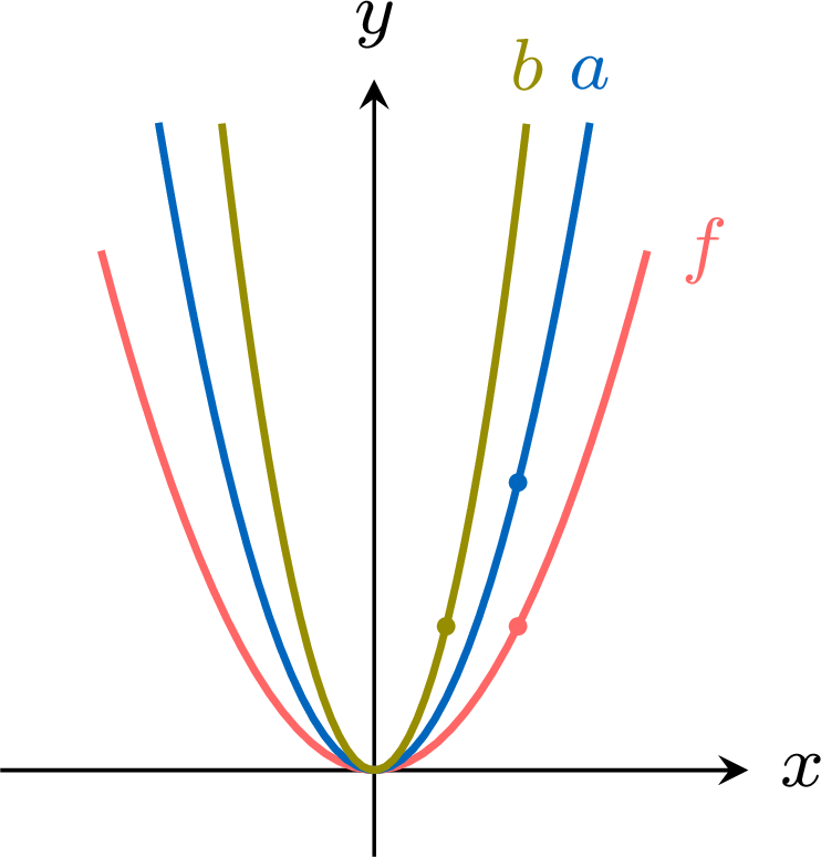
From the graph of \(f(x) = x^2\), plot \(a(x) = 2f(x)\) and \(b(x) = f(2x)\). - \(a(x) = 2f(x) = 2x^2\): every output is doubled — a vertical stretch with scale factor \(2\). The point \((1, 1)\) moves to \((1, 2)\).
- \(b(x) = f(2x) = 4x^2\): the input is consumed twice as fast — a horizontal stretch with scale factor \(\frac12\), a compression: every \(x\)-coordinate is halved. The point \((1, 1)\) moves to \(\left(\frac12, 1\right)\).
Stretches and Scale Factors
The number by which a stretch multiplies the distances to the axis that stays fixed is its scale factor. For \(a > 0\), the graph of \(y = a f(x)\) is the image of the graph of \(y = f(x)\) under the vertical stretch with scale factor \(a\): each point \((x, y)\) goes to \((x, ay)\). For \(b > 0\), the graph of \(y = f(bx)\) is its image under the horizontal stretch with scale factor \(\dfrac{1}{b}\): each point \((x, y)\) goes to \(\left(\dfrac{x}{b}, y\right)\). A scale factor greater than \(1\) moves the points away from the axis that stays fixed (the \(x\)-axis for a vertical stretch, the \(y\)-axis for a horizontal one), a scale factor between \(0\) and \(1\) brings them closer to it: the graph of \(y = f(2x)\) is the image of the graph of \(f\) under the horizontal stretch with scale factor \(\dfrac{1}{2}\), a compression.
Skills to practice
- Stretching Graphs
I.3
Reflections
Recappreviously studied — click to reread
Definition — Reflection in the x-axis
A reflection in the x-axis flips the graph of a function vertically. It is a special case of vertical stretch where \(a=-1\). It is defined by:$$g(x) = -f(x)$$ This transformation maps a point \((x, y)\) to \((x, -y)\). 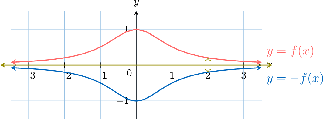
Definition — Reflection in the y-axis
A reflection in the y-axis flips the graph of a function horizontally. It is a special case of horizontal stretch where \(b=-1\). It is defined by:$$g(x) = f(-x)$$ This transformation maps a point \((x, y)\) to \((-x, y)\). 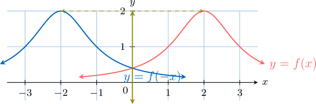
Example
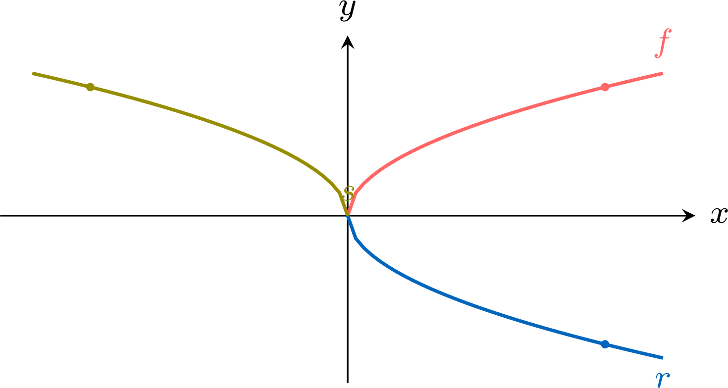
From the graph of \(f(x) = \sqrt{x}\), plot \(r(x) = -f(x)\) and \(s(x) = f(-x)\). - \(r(x) = -\sqrt{x}\): every output changes sign — a reflection in the \(x\)-axis. The curve flips below the axis; the point \((4, 2)\) moves to \((4, -2)\).
- \(s(x) = \sqrt{-x}\): every input changes sign — a reflection in the \(y\)-axis. The curve flips to the left half-plane (defined for \(x \le 0\)); the point \((4, 2)\) moves to \((-4, 2)\).
Skills to practice
- Reflecting Graphs
II
Composite Transformations
II.1
Combining Transformations
Recappreviously studied — click to reread
When several transformations are applied to a function, the order can matter between two horizontal transformations, or between two vertical ones (a stretch and a translation, for example); a horizontal transformation and a vertical one can be applied in either order. The standard form for a transformed function is:$$ g(x) = a \cdot f(b(x-c)) + d $$ To graph this function from the parent function \(f(x)\), apply the transformations in the following order:
Method — Order of Transformations
- Horizontal Transformations (inside the brackets):
- Apply the horizontal stretch with scale factor \(\frac{1}{|b|}\) (\(b \neq 0\)), followed by a reflection in the \(y\)-axis if \(b < 0\).
- Apply the horizontal translation (shift) by \(c\) units.
- Vertical Transformations (outside the brackets):
- Apply the vertical stretch with scale factor \(|a|\), followed by a reflection in the \(x\)-axis if \(a < 0\).
- Apply the vertical translation (shift) by \(d\) units.
Example
Describe the sequence of transformations that maps the graph of \(f(x)=\sqrt{x}\) onto the graph of \(g(x) = 3\sqrt{-x+2} - 4\).
First, we rewrite the function \(g(x)\) in the standard form \(a \cdot f(b(x-c)) + d\):$$ g(x) = 3\sqrt{-(x-2)} - 4 $$ Comparing this to \(f(x)=\sqrt{x}\), we have \(a=3\), \(b=-1\), \(c=2\), and \(d=-4\). The transformations are applied as follows: 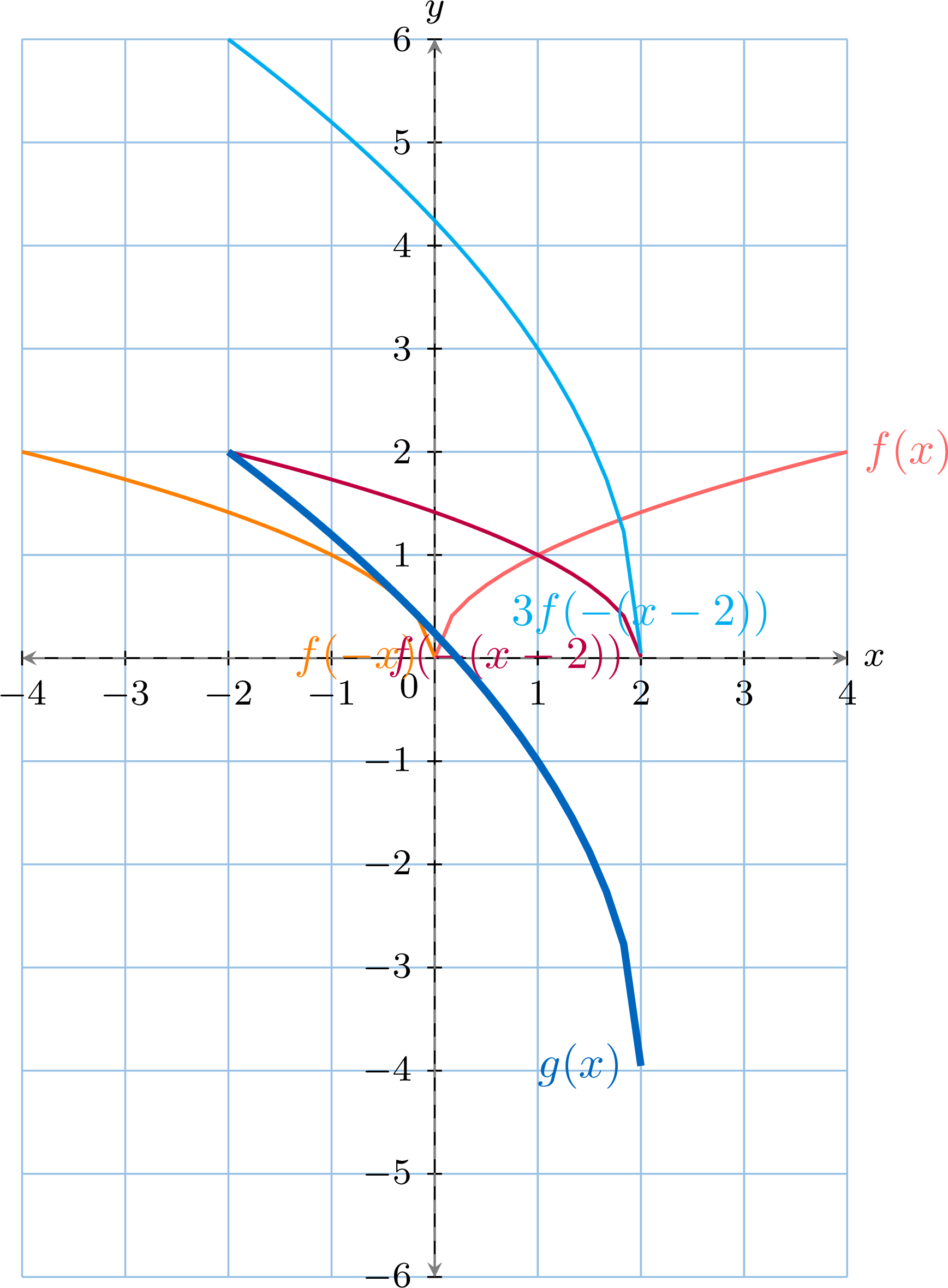
- Horizontal Transformations on \(f(x)=\sqrt{x}\):
- Reflection: Since \(b=-1\), reflect the graph in the y-axis (\(y = \sqrt{-x}\)).
- Translation: Since \(c=2\), translate the graph 2 units to the right (\(y = \sqrt{-(x-2)}\)).
- Vertical Transformations on the result:
- Stretch: Since \(a=3\), stretch the graph vertically with scale factor 3 (\(y = 3\sqrt{-(x-2)}\)).
- Translation: Since \(d=-4\), translate the graph 4 units down (\(y = 3\sqrt{-(x-2)} - 4\)).
Example
The graph of \(y = f(x)\) is reflected in the \(y\)-axis, then stretched horizontally with scale factor \(2\). Find an equation of the image, and check it with a point \((a, b)\) of the graph of \(f\).
Each transformation acts on the equation obtained at the previous step: a horizontal transformation replaces \(x\) in the current expression, a vertical transformation acts on the whole current expression.
Check with a point. The reflection sends a point \((a, b)\) of the graph of \(f\) to \((-a, b)\), and the stretch doubles the \(x\)-coordinate: \((-a, b)\) goes to \((-2a, b)\). At \(x = -2a\), the expression inside \(f\) is $$\begin{aligned}[t] -\frac{x}{2} &= -\frac{-2a}{2} && (x = -2a) \\ &= a, \end{aligned}$$ so \(f\left(-\dfrac{x}{2}\right) = f(a) = b\), since the point \((a, b)\) is on the graph of \(f\): the point \((-2a, b)\) is indeed on the image. Replacing \(x\) by \(-2x\) instead, that is writing \(f(-2x)\), would give the horizontal stretch with scale factor \(\dfrac{1}{2}\): the check with a point detects this error, since \(f\big(-2 \times (-2a)\big) = f(4a)\) is not equal to \(b\) in general. 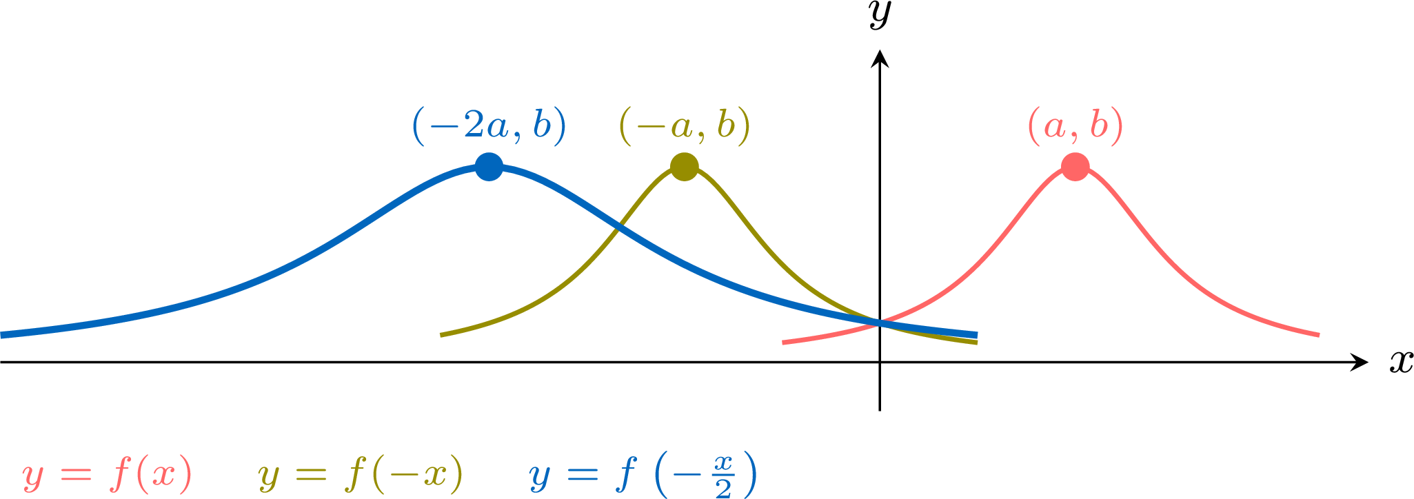
- Reflection in the \(y\)-axis: \(x\) is replaced by \(-x\): \(y = f(-x)\).
- Horizontal stretch with scale factor \(2\): \(x\) is replaced by \(\dfrac{x}{2}\) in the current expression \(f(-x)\): \(y = f\left(-\dfrac{x}{2}\right)\).
Check with a point. The reflection sends a point \((a, b)\) of the graph of \(f\) to \((-a, b)\), and the stretch doubles the \(x\)-coordinate: \((-a, b)\) goes to \((-2a, b)\). At \(x = -2a\), the expression inside \(f\) is $$\begin{aligned}[t] -\frac{x}{2} &= -\frac{-2a}{2} && (x = -2a) \\ &= a, \end{aligned}$$ so \(f\left(-\dfrac{x}{2}\right) = f(a) = b\), since the point \((a, b)\) is on the graph of \(f\): the point \((-2a, b)\) is indeed on the image. Replacing \(x\) by \(-2x\) instead, that is writing \(f(-2x)\), would give the horizontal stretch with scale factor \(\dfrac{1}{2}\): the check with a point detects this error, since \(f\big(-2 \times (-2a)\big) = f(4a)\) is not equal to \(b\) in general.
Skills to practice
- Sketching Combined Transformations
- Finding Equations after a Sequence of Transformations
II.2
Rational Functions as Images of \(y \equal \frac{1}{x}\)
A function of the form \(y = \dfrac{ax + b}{cx + d}\), with \(c \neq 0\) and \(ad - bc \neq 0\), can be rewritten as \(y = p + \dfrac{q}{x - h}\) by writing the numerator around the denominator. Its graph is then the image of the graph of \(y = \dfrac{1}{x}\) under a sequence of translations, stretches and reflections, and its asymptotes are the images of the two axes.
Example
Describe a sequence of transformations that maps the graph of \(y = \dfrac{1}{x}\) onto the graph of \(y = \dfrac{2x + 1}{x - 1}\), and deduce the asymptotes of the second graph.
Write the numerator around the denominator: \(2x + 1 = 2(x - 1) + 3\). With \(f(x) = \dfrac{1}{x}\), for \(x \neq 1\): $$\begin{aligned}[t] \frac{2x + 1}{x - 1} &= \frac{2(x - 1) + 3}{x - 1} \\
&= 2 + \frac{3}{x - 1} && \text{(split the fraction)} \\
&= 3f(x - 1) + 2. \end{aligned}$$ This is the standard form \(a \cdot f(b(x - c)) + d\) with \(a = 3\), \(b = 1\), \(c = 1\) and \(d = 2\). In the order of transformations: 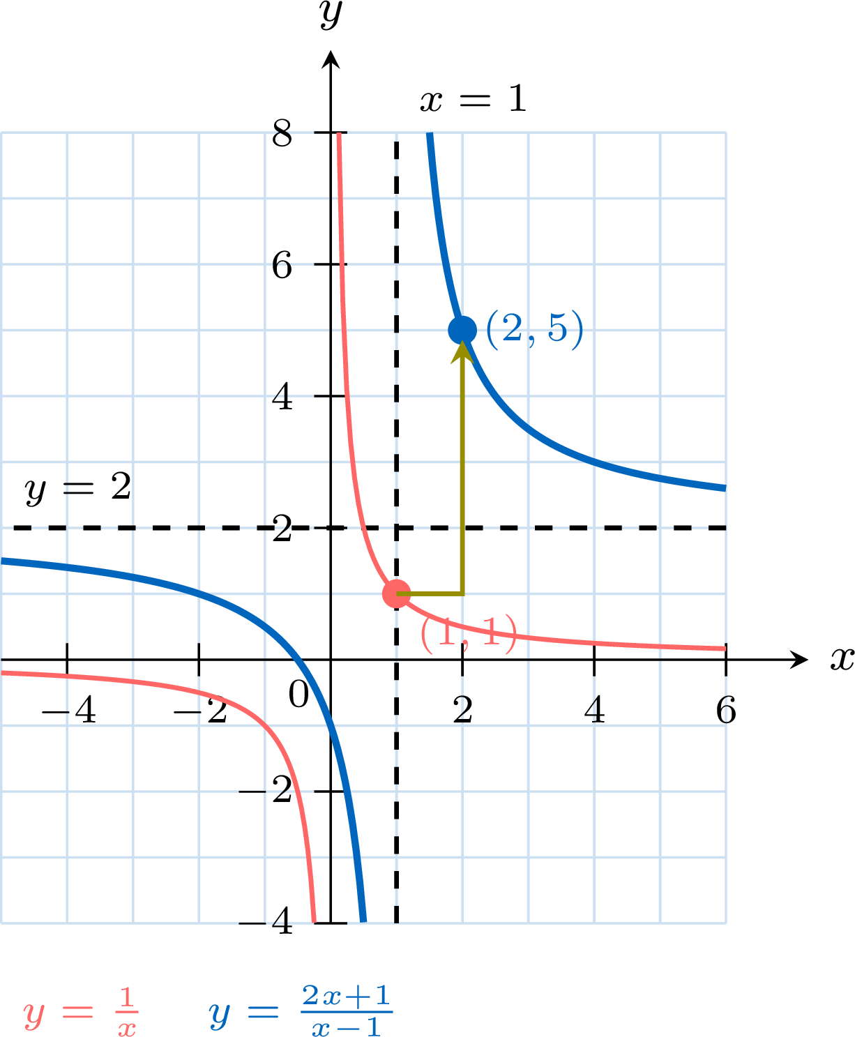
- translate \(1\) unit to the right: \(y = \dfrac{1}{x - 1}\);
- stretch vertically with scale factor \(3\): \(y = \dfrac{3}{x - 1}\);
- translate \(2\) units up: \(y = \dfrac{3}{x - 1} + 2\).
Skills to practice
- Relating Rational Functions to \(y \equal \frac{1}{x}\)
III
The Graph of \(y \equal \frac{1}{f(x)}\)
III.1
Reciprocal Graphs
Let \(f(x) = x^2 - 4\). Whenever \(f(x) \neq 0\), the number \(f(x)\) has a reciprocal \(\dfrac{1}{f(x)}\): how does the graph of \(y = \dfrac{1}{f(x)}\) compare with the graph of \(f\)?
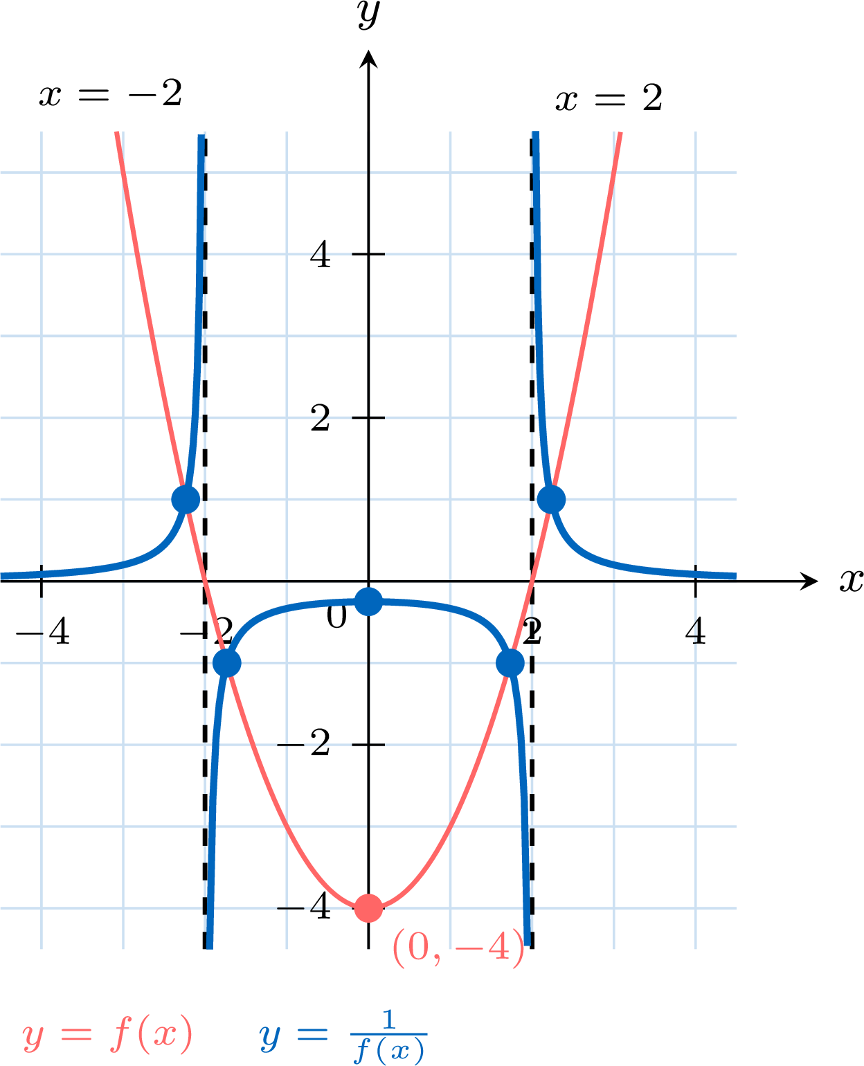
The graph of \(y = \dfrac{1}{f(x)}\) has three branches, separated by the vertical asymptotes \(x = -2\) and \(x = 2\); the minimum point \((0, -4)\) of \(f\) has become the highest point \(\left(0, -\dfrac{1}{4}\right)\) of the middle branch. The Propositions “Sign, Invariant Points and Variations” and “Asymptotes of the Graph of \(y = \dfrac{1}{f(x)}\)” turn each of these observations into a rule.
- Compute \(f(x)\) and \(\dfrac{1}{f(x)}\) for \(x = 0\), \(1\), \(3\) and \(4\). Why are the values the same for \(x = -1\), \(-3\) and \(-4\)?
- Why can \(\dfrac{1}{f(x)}\) not be computed for \(x = 2\) and for \(x = -2\)? What happens to \(\dfrac{1}{f(x)}\) when \(x\) gets closer and closer to \(2\)?
- What happens to \(\dfrac{1}{f(x)}\) when \(x\) becomes large?
- For which values of \(x\) are the two numbers \(f(x)\) and \(\dfrac{1}{f(x)}\) equal?
- The values:
\(x\) \(0\) \(1\) \(3\) \(4\) \(f(x) = x^2 - 4\) \(-4\) \(-3\) \(5\) \(12\) \(\dfrac{1}{f(x)}\) \(-\dfrac{1}{4}\) \(-\dfrac{1}{3}\) \(\dfrac{1}{5}\) \(\dfrac{1}{12}\) - \(f(2) = f(-2) = 0\), and \(0\) has no reciprocal. Close to \(2\), \(f(x)\) is close to \(0\): \(f(2.1) = 0.41\), \(f(2.01) = 0.0401\) and \(f(1.99) = -0.0399\), so \(\dfrac{1}{f(2.1)} \approx 2.44\), \(\dfrac{1}{f(2.01)} \approx 24.9\) and \(\dfrac{1}{f(1.99)} \approx -25.1\). The absolute values \(\left|\dfrac{1}{f(x)}\right|\) become as large as desired: the line \(x = 2\) is a vertical asymptote of the graph of \(y = \dfrac{1}{f(x)}\), and so is the line \(x = -2\).
- When \(x\) becomes large, \(f(x) = x^2 - 4\) becomes as large as desired, so \(\dfrac{1}{f(x)}\) gets as close to \(0\) as desired: the \(x\)-axis is a horizontal asymptote.
- For \(f(x) \neq 0\): $$\begin{aligned}[t] f(x) = \frac{1}{f(x)} &\iff f(x)^2 = 1 && \text{(multiply by } f(x) \neq 0\text{)} \\ &\iff f(x) = 1 \ \text{ or } \ f(x) = -1 \\ &\iff x^2 = 5 \ \text{ or } \ x^2 = 3 && (f(x) = x^2 - 4) \\ &\iff x = \pm\sqrt{5} \ \text{ or } \ x = \pm\sqrt{3}. \end{aligned}$$ The two graphs meet at four points, on the lines \(y = 1\) and \(y = -1\).
Definition — The Reciprocal of a Function
Let \(f\) be a function. The reciprocal of \(f\) is the function \(\dfrac{1}{f}\) given by $$\frac{1}{f}(x) = \frac{1}{f(x)}.$$ It is defined for every \(x\) of the domain of \(f\) such that \(f(x) \neq 0\). Its graph is the graph of the equation \(y = \dfrac{1}{f(x)}\). A point lying on both the graph of \(f\) and the graph of \(y = \dfrac{1}{f(x)}\) is an invariant point.The reciprocal \(\dfrac{1}{f}\) must not be confused with the inverse function \(f^{-1}\), which undoes \(f\): for \(f(x) = 2x\), \(\dfrac{1}{f(x)} = \dfrac{1}{2x}\), whereas \(f^{-1}(x) = \dfrac{x}{2}\).
Proposition — Sign, Invariant Points and Variations
Let \(f\) be a function. - Sign: wherever \(f(x) \neq 0\), the number \(\dfrac{1}{f(x)}\) has the same sign as \(f(x)\). The graphs of \(y = f(x)\) and \(y = \dfrac{1}{f(x)}\) lie on the same side of the \(x\)-axis.
- Invariant points: a point lies on both graphs exactly when it is a point of the graph of \(f\) at which \(f(x) = 1\) or \(f(x) = -1\). The two graphs meet only on the lines \(y = 1\) and \(y = -1\).
- Variations: on an interval where \(f(x)\) is never \(0\) and keeps the same sign, if \(f\) is increasing then \(\dfrac{1}{f}\) is decreasing, and if \(f\) is decreasing then \(\dfrac{1}{f}\) is increasing.
- Maximum and minimum: on such an interval, if \(f(a)\) is the maximum of \(f\), then \(\dfrac{1}{f(a)}\) is the minimum of \(\dfrac{1}{f}\), and if \(f(a)\) is the minimum of \(f\), then \(\dfrac{1}{f(a)}\) is the maximum of \(\dfrac{1}{f}\). So, when the graph of \(f\) has no break near \(a\) (then \(f(x)\) keeps the sign of \(m\) for \(x\) close to \(a\)), a local maximum point \((a, m)\) of the graph of \(f\), with \(m \neq 0\), becomes a local minimum point \(\left(a, \dfrac{1}{m}\right)\) of the graph of \(y = \dfrac{1}{f(x)}\), and a local minimum point becomes a local maximum point.
- Sign. \(f(x) \times \dfrac{1}{f(x)} = 1 > 0\): the two numbers are nonzero and have the same sign.
- Invariant points. The point with \(x\)-coordinate \(x\) lies on both graphs when \(f(x) = \dfrac{1}{f(x)}\), with \(f(x) \neq 0\): $$\begin{aligned}[t] f(x) = \frac{1}{f(x)} &\iff f(x)^2 = 1 && \text{(multiply by } f(x) \neq 0\text{)} \\ &\iff f(x) = 1 \ \text{ or } \ f(x) = -1. \end{aligned}$$
- Variations. Let \(u \leq v\) be two numbers of an interval \(I\) on which \(f(x)\) is never \(0\) and keeps the same sign. Then \(f(u) f(v) > 0\), and $$\begin{aligned}[t] \frac{1}{f(u)} - \frac{1}{f(v)} &= \frac{f(v) - f(u)}{f(u) f(v)}. && \text{(common denominator)} \end{aligned}$$ If \(f\) is increasing, \(f(v) - f(u) \geq 0\), so \(\dfrac{1}{f(u)} \geq \dfrac{1}{f(v)}\): \(\dfrac{1}{f}\) is decreasing on \(I\). If \(f\) is decreasing, \(f(v) - f(u) \leq 0\) and \(\dfrac{1}{f}\) is increasing on \(I\).
- Maximum and minimum. If \(f(a)\) is the maximum of \(f\) on \(I\), then \(f(x) \leq f(a)\) for every \(x\) of \(I\), and \(f(x) f(a) > 0\), so $$\frac{1}{f(x)} - \frac{1}{f(a)} = \frac{f(a) - f(x)}{f(x) f(a)} \geq 0:$$ \(\dfrac{1}{f(a)}\) is the minimum of \(\dfrac{1}{f}\) on \(I\). The case of a minimum is the same with the inequalities reversed. When the graph of \(f\) has no break at \(a\) and \(f(a) = m \neq 0\), \(f(x)\) keeps the sign of \(m\) on an interval around \(a\), on which this applies: a local maximum point of the graph of \(f\) becomes a local minimum point, and conversely.
Proposition — Asymptotes of the Graph of \(y \equal \frac{1}{f(x)}\)
Let \(f\) be a function whose graph has no break, except at its vertical asymptotes. - Zeros become vertical asymptotes: if \(f(a) = 0\), the graph of \(f\) has no break at \(a\), and \(f(x) \neq 0\) for the other values of \(x\) close to \(a\), the line \(x = a\) is a vertical asymptote of the graph of \(y = \dfrac{1}{f(x)}\).
- Large values become values close to \(0\): where \(|f(x)|\) becomes as large as desired, \(\dfrac{1}{f(x)}\) gets as close to \(0\) as desired. So if \(|f(x)|\) becomes as large as desired when \(x\) becomes large, the \(x\)-axis is a horizontal asymptote of the graph of \(y = \dfrac{1}{f(x)}\); and if the line \(x = p\) is a vertical asymptote of the graph of \(f\), the graph of \(y = \dfrac{1}{f(x)}\) comes as close as desired to the point \((p, 0)\), which does not belong to it, since a reciprocal \(\dfrac{1}{f(x)}\) is never \(0\): this point is drawn as an open circle.
- Horizontal asymptotes: if the line \(y = q\), with \(q \neq 0\), is a horizontal asymptote of the graph of \(f\), the line \(y = \dfrac{1}{q}\) is a horizontal asymptote of the graph of \(y = \dfrac{1}{f(x)}\).
- Zeros. Since the graph of \(f\) has no break at \(a\) and \(f(a) = 0\), \(f(x)\) gets as close to \(0\) as desired when \(x\) gets close to \(a\), without being \(0\) for \(x \neq a\). Then \(\left|\dfrac{1}{f(x)}\right| = \dfrac{1}{|f(x)|}\) becomes as large as desired: by the definition of a vertical asymptote, the line \(x = a\) is one.
- Large values. If \(|f(x)|\) is larger than a number \(M > 0\), then \(\left|\dfrac{1}{f(x)}\right| = \dfrac{1}{|f(x)|}\) is smaller than \(\dfrac{1}{M}\), which is as small as desired when \(M\) is large enough.
- Horizontal asymptotes. Suppose \(f(x)\) gets as close to \(q \neq 0\) as desired when \(x\) becomes large. Once \(f(x)\) is within \(\dfrac{|q|}{2}\) of \(q\), \(|f(x)| \geq \dfrac{|q|}{2}\), and $$\left|\frac{1}{f(x)} - \frac{1}{q}\right| = \frac{|q - f(x)|}{|q| \, |f(x)|} \leq \frac{2}{q^2}\,|q - f(x)|,$$ which gets as close to \(0\) as desired: \(\dfrac{1}{f(x)}\) gets as close to \(\dfrac{1}{q}\) as desired, and the line \(y = \dfrac{1}{q}\) is a horizontal asymptote.
Method — Sketching the Graph of \(y \equal \frac{1}{f(x)}\) from the Graph of \(y \equal f(x)\)
- Draw the vertical asymptotes: the lines \(x = a\) at the zeros \(a\) of \(f\) (each zero \(a\) such that \(f(x) \neq 0\) for the other values of \(x\) close to \(a\)).
- Mark the invariant points, where the graph of \(f\) meets the lines \(y = 1\) and \(y = -1\).
- Turn each turning point \((a, m)\) of \(f\), with \(m \neq 0\) and the graph of \(f\) without a break near \(a\), into \(\left(a, \dfrac{1}{m}\right)\), a maximum becoming a minimum and a minimum a maximum; mark the \(y\)-intercept \(\left(0, \dfrac{1}{f(0)}\right)\) when \(f(0) \neq 0\).
- Where \(|f(x)|\) becomes large, draw \(\dfrac{1}{f(x)}\) close to \(0\): the \(x\)-axis as a horizontal asymptote, or an open circle at \((p, 0)\) for a vertical asymptote \(x = p\) of \(f\). A horizontal asymptote \(y = q \neq 0\) of \(f\) gives the horizontal asymptote \(y = \dfrac{1}{q}\).
- Join the points on each interval between the asymptotes, leaving out the open circles, keeping the sign of \(f\) and reversing its variations: where \(f\) increases, \(\dfrac{1}{f}\) decreases, and where \(f\) decreases, \(\dfrac{1}{f}\) increases.
- The range of \(\dfrac{1}{f}\) is made of the numbers \(\dfrac{1}{y}\), for the nonzero values \(y\) taken by \(f\).
Example
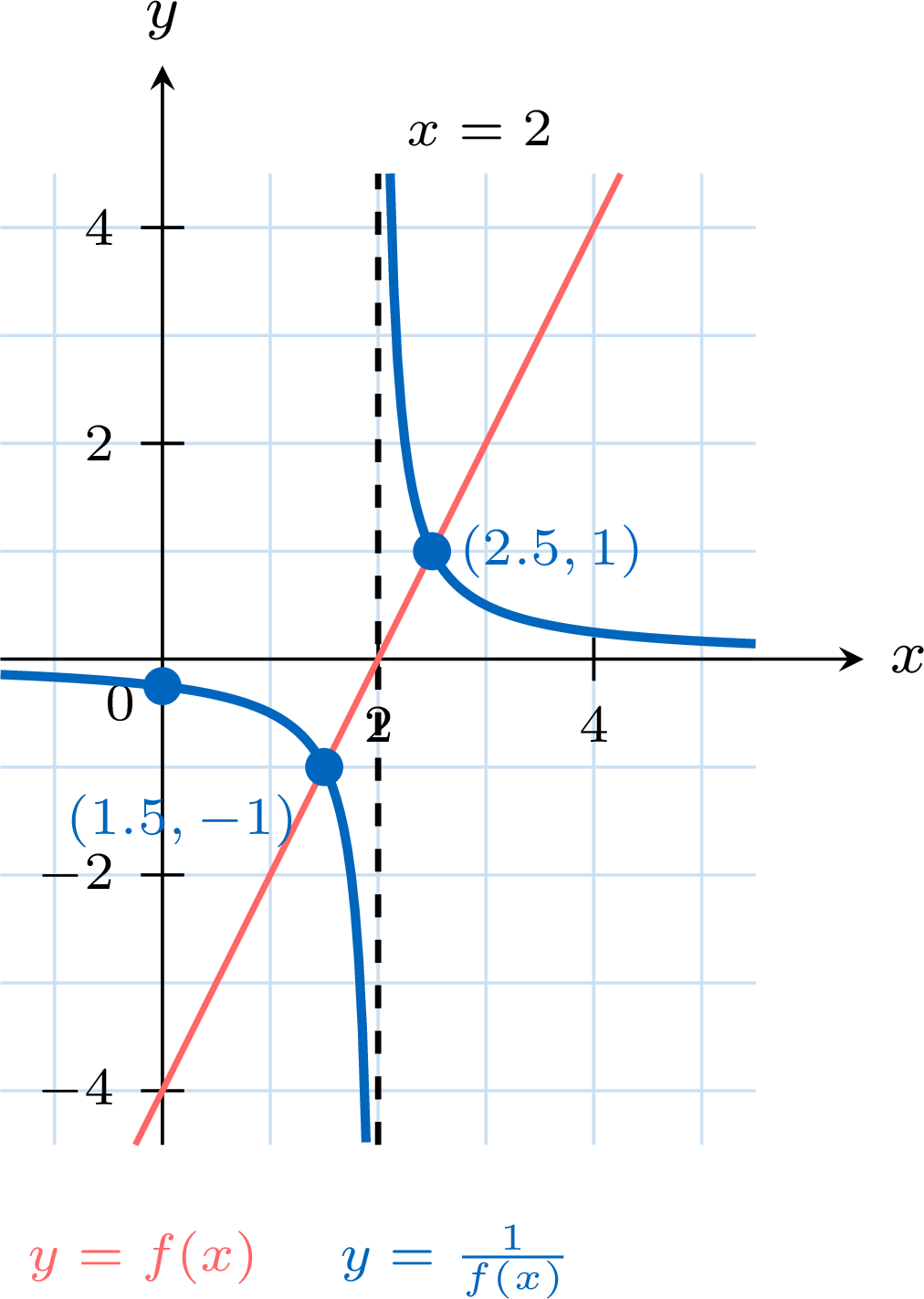
Sketch the graph of \(y = \dfrac{1}{2x - 4}\) from the graph of \(f(x) = 2x - 4\). - Vertical asymptote. \(2x - 4 = 0\) for \(x = 2\): the line \(x = 2\).
- Invariant points. \(2x - 4 = 1\) for \(x = \dfrac{5}{2}\), and \(2x - 4 = -1\) for \(x = \dfrac{3}{2}\): the points \(\left(\dfrac{5}{2}, 1\right)\) and \(\left(\dfrac{3}{2}, -1\right)\).
- Intercept. \(\dfrac{1}{f(0)} = \dfrac{1}{-4} = -\dfrac{1}{4}\): the point \(\left(0, -\dfrac{1}{4}\right)\). A line that is not horizontal has no turning point.
- Large values. \(|2x - 4|\) becomes as large as desired when \(x\) becomes large: the \(x\)-axis is a horizontal asymptote.
- Sign and variations. \(f\) is increasing, negative for \(x < 2\) and positive for \(x > 2\): \(\dfrac{1}{f}\) is decreasing on each of the two intervals. The left branch lies below the \(x\)-axis and falls along \(x = 2\); the right branch lies above it and comes down from the top along \(x = 2\).
Example
The graph of a quadratic function \(f\) is shown: it cuts the \(x\)-axis at \(-1\) and \(3\), and its vertex is \((1, -4)\). Sketch the graph of \(y = \dfrac{1}{f(x)}\). 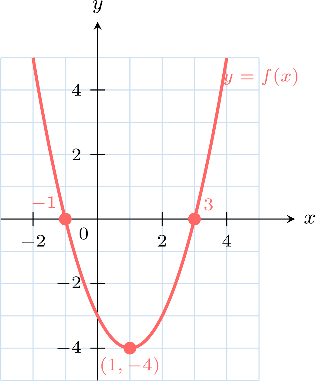
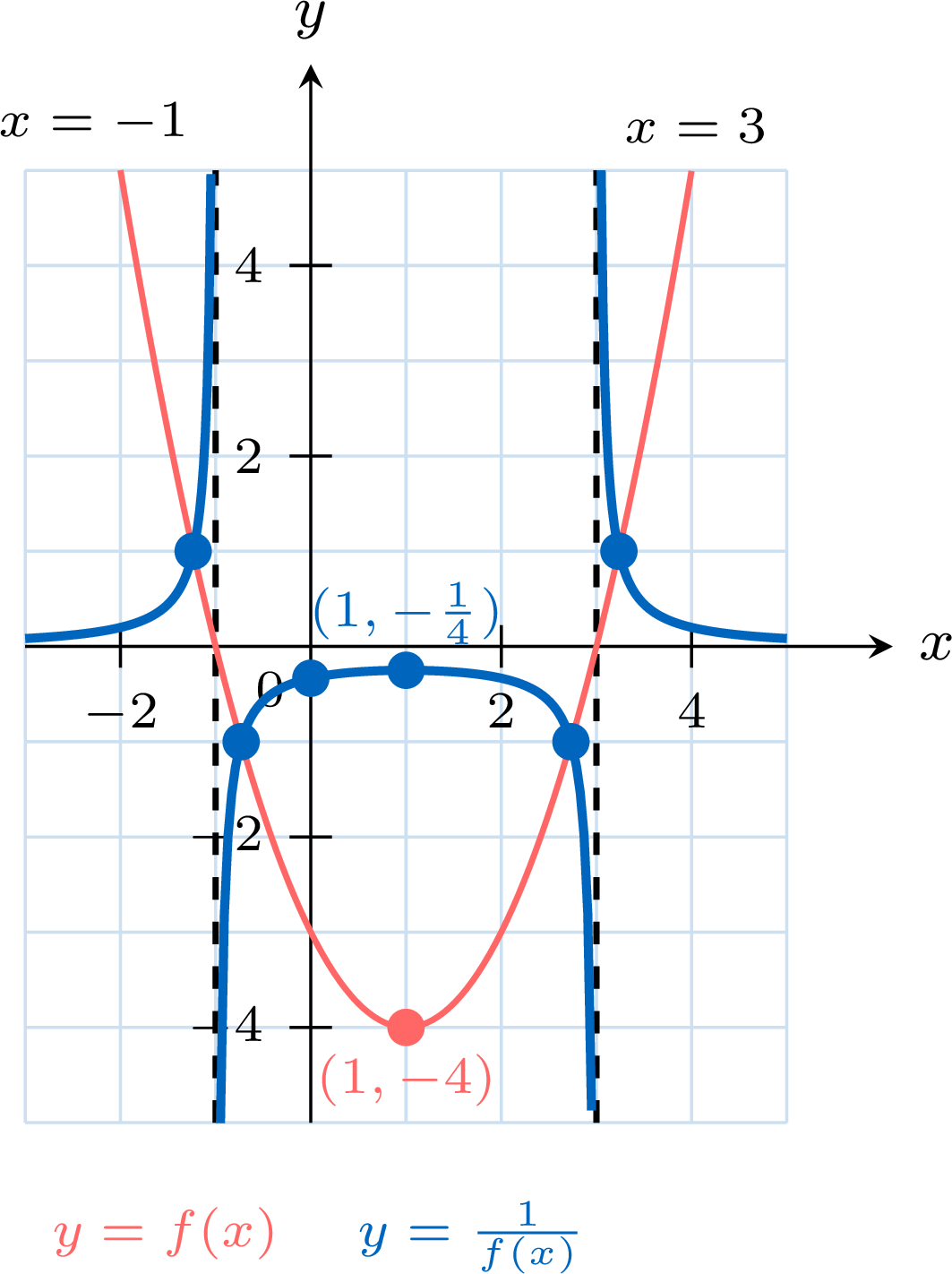
- Vertical asymptotes. The zeros of \(f\) are \(-1\) and \(3\): the lines \(x = -1\) and \(x = 3\).
- Turning point. The vertex \((1, -4)\) is the minimum point of \(f\), with \(-4 \neq 0\): it becomes the local maximum point \(\left(1, -\dfrac{1}{4}\right)\).
- Invariant points. The parabola meets each of the lines \(y = 1\) and \(y = -1\) at two points, which lie on both graphs. With the formula \(f(x) = (x + 1)(x - 3)\), found from the intercepts and the vertex (the coefficient \(a\) of \(f(x) = a(x + 1)(x - 3)\) satisfies \(f(1) = -4a = -4\), so \(a = 1\)), their \(x\)-coordinates are \(1 \pm \sqrt{5}\) and \(1 \pm \sqrt{3}\). The \(y\)-intercept \(f(0) = -3\) gives the point \(\left(0, -\dfrac{1}{3}\right)\).
- Large values. \(f(x)\) becomes as large as desired when \(x\) becomes large: the \(x\)-axis is a horizontal asymptote.
- Sign and variations. \(f(x) > 0\) for \(x < -1\) and for \(x > 3\), \(f(x) < 0\) between \(-1\) and \(3\). The outer branches lie above the \(x\)-axis and climb along the asymptotes; the middle branch lies below it, rises from the bottom along \(x = -1\) to its highest point \(\left(1, -\dfrac{1}{4}\right)\), then falls along \(x = 3\).
Example
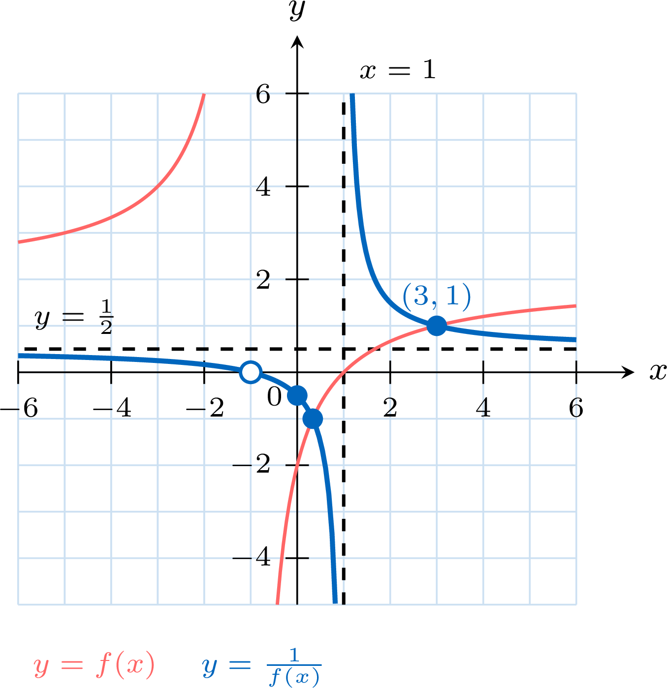
The graph of \(f(x) = \dfrac{2x - 2}{x + 1}\) is shown, with its asymptotes \(x = -1\) and \(y = 2\); it passes through \((1, 0)\) and \((0, -2)\). Give the domain of \(\dfrac{1}{f}\) and sketch the graph of \(y = \dfrac{1}{f(x)}\). 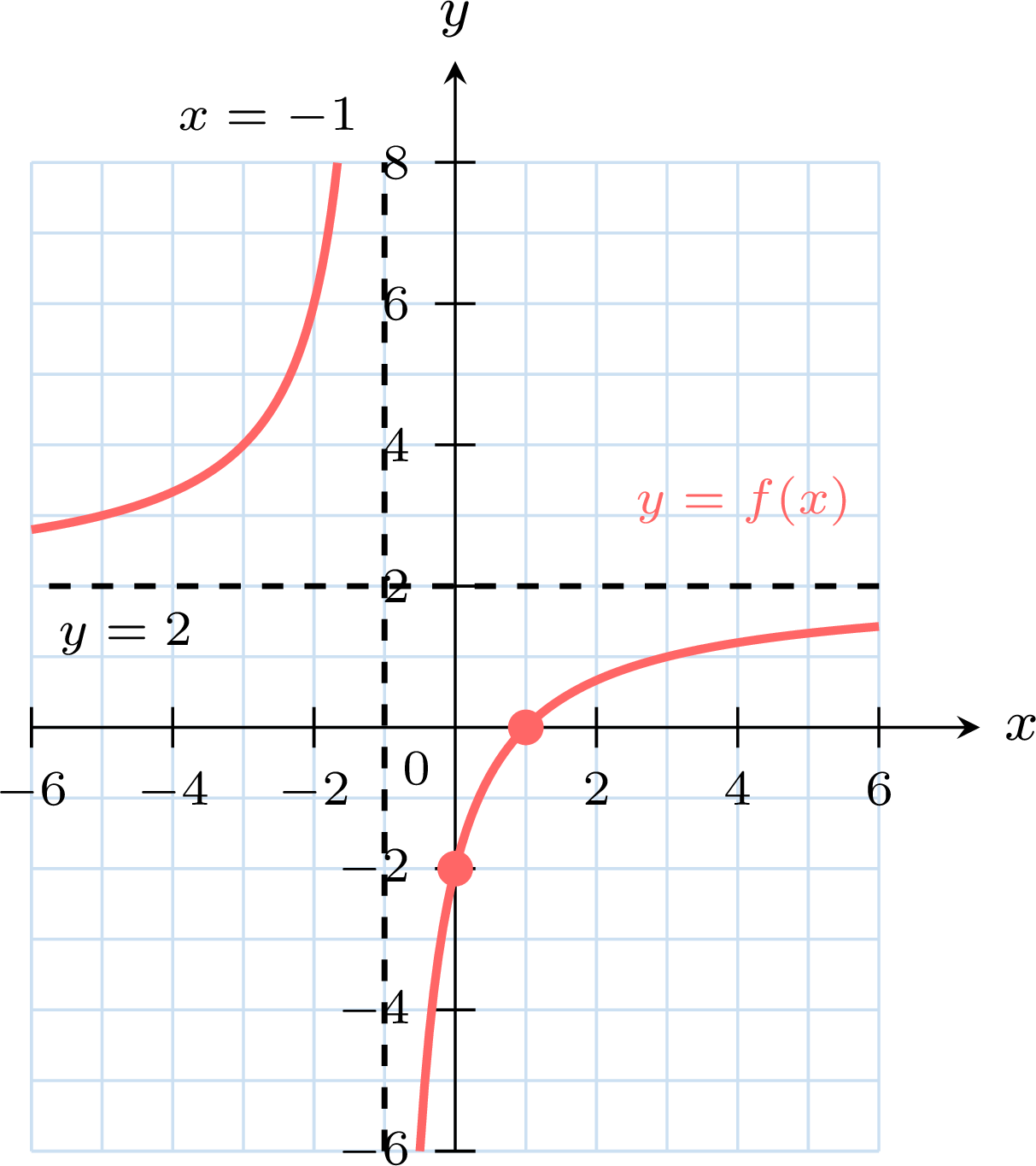
- Domain. \(\dfrac{1}{f(x)}\) needs \(f(x)\) to be defined, so \(x \neq -1\), and nonzero, so \(x \neq 1\): the domain is \(\mathbb{R} \setminus \{-1, 1\}\).
- Asymptotes. The zero \(1\) of \(f\) gives the vertical asymptote \(x = 1\). The horizontal asymptote \(y = 2\) of \(f\) gives the horizontal asymptote \(y = \dfrac{1}{2}\). The vertical asymptote \(x = -1\) of \(f\) gives the open circle \((-1, 0)\): the graph comes as close as desired to this point, which does not belong to it.
- Points. \(f(x) = 1\) when \(2x - 2 = x + 1\), that is \(x = 3\); \(f(x) = -1\) when \(2x - 2 = -x - 1\), that is \(x = \dfrac{1}{3}\): the invariant points are \((3, 1)\) and \(\left(\dfrac{1}{3}, -1\right)\). The \(y\)-intercept is \(\dfrac{1}{f(0)} = -\dfrac{1}{2}\).
- Check. For \(x \neq \pm 1\), \(\dfrac{1}{f(x)} = \dfrac{x + 1}{2x - 2}\), a rational function whose asymptotes are \(x = 1\) and \(y = \dfrac{1}{2}\), as found; the graph of \(y = \dfrac{1}{f(x)}\) is the graph of this rational function without its point \((-1, 0)\), where \(f\) is not defined.
Example
Let \(f(x) = x^3 - 4x + 1\). Use technology to find the vertical asymptotes and the turning points of the graph of \(y = \dfrac{1}{f(x)}\), to \(3\) significant figures, and sketch it.
Enter \(Y_1 = x^3 - 4x + 1\) in the window \(-3 \le x \le 3\), \(-5 \le y \le 6\), and read its key features with the analysis tools (Method “Reading the Key Features of a Graph on the Screen”). 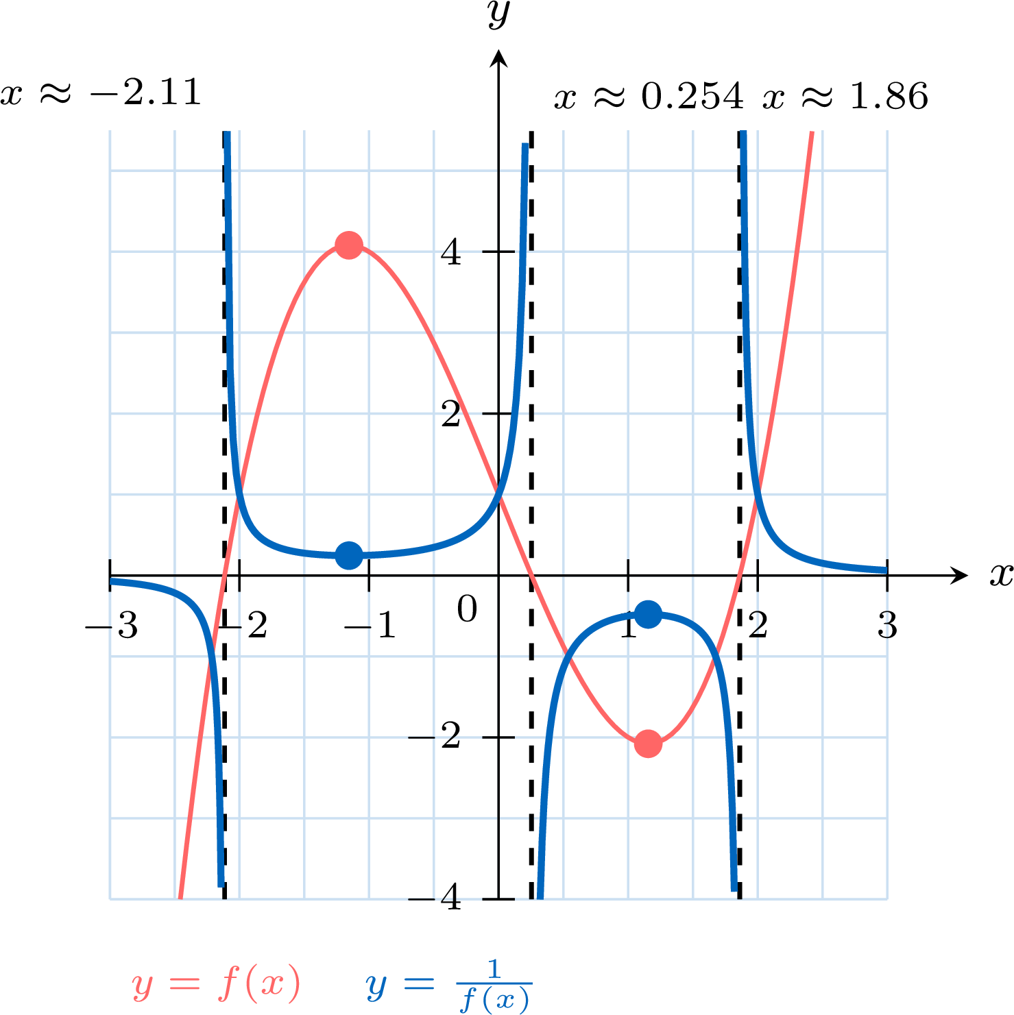
- Vertical asymptotes. The tool zero displays \(X = -2.1149075\), \(X = 0.25410169\) and \(X = 1.8608059\): the vertical asymptotes are \(x \approx -2.11\), \(x \approx 0.254\) and \(x \approx 1.86\).
- Turning points. The tool maximum displays \(X = -1.1547005\), \(Y = 4.0792014\), and the tool minimum \(X = 1.1547005\), \(Y = -2.0792014\). The local maximum of \(f\) becomes a local minimum of \(\dfrac{1}{f}\), with value \(\dfrac{1}{4.0792014} \approx 0.245\), and the local minimum becomes a local maximum, with value \(\dfrac{1}{-2.0792014} \approx -0.481\): the turning points are \((-1.15, 0.245)\) and \((1.15, -0.481)\).
- Check on the screen. With \(Y_2 = \dfrac{1}{Y_1}\), the tools minimum and maximum applied to \(Y_2\) give the same two points. The calculator may join two branches across an asymptote with an almost vertical segment, which is not part of the graph.
Skills to practice
- Recognising Features of the Graph of \(y \equal \frac{1}{f(x)}\)
- Finding Asymptotes and Invariant Points
- Studying \(y \equal \frac{1}{f(x)}\) with Technology
- Sketching the Graph of \(y \equal \frac{1}{f(x)}\)
IV
Going further
Skills to practice
- Reasoning about Transformations
- Solving Problems with Transformations
- Reasoning about Reciprocal Graphs
- Solving Problems with Reciprocal Graphs
- Quiz
Jump to section