International Baccalaureate · DP 1: Analysis and Approaches SL
Descriptive Statistics
I
Measuring the Centre
I.1
Measures of Centre
Recappreviously studied — click to reread
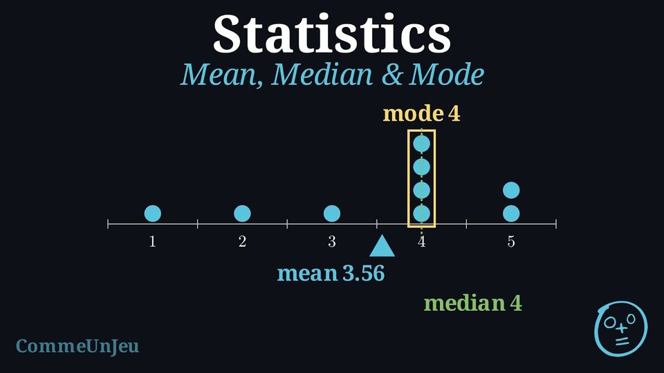
Definition — Mode
The mode is the value or category that appears most frequently. A dataset can have more than one mode. When every value appears the same number of times, the data are said to have no mode. Definition — Mean
The mean is the sum of all numerical values divided by the count of values. It is often called the “average”.$$\begin{aligned} \bar{x} &= \frac{\text{sum of all values}}{\text{number of values}} \\
&= \frac{x_1 + x_2 + x_3 + \dots + x_n}{n}\end{aligned}$$ Definition — Median
The median is the middle value of a dataset that has been ordered from least to greatest. - If there is an odd number of values, the median is the single middle value.
- If there is an even number of values, there are two middle values and the median is the mean of these two values.
Definition — Mean from a Frequency Table
When a value \(x_i\) is repeated \(n_i\) times (its frequency), it is wasteful to add it \(n_i\) times one by one. The mean is then computed as a weighted mean: each distinct value is weighted by its frequency. $$ \bar{x} = \frac{n_1 x_1 + n_2 x_2 + \dots + n_k x_k}{n_1 + n_2 + \dots + n_k} = \frac{\sum_{i=1}^{k} n_i x_i}{N} $$ where \(x_1, x_2, \dots, x_k\) are the \(k\) distinct values, \(n_i\) is the frequency of \(x_i\), and \(N = \sum_{i=1}^{k} n_i\) is the total number of data values. The symbol \(\sum\) means “sum over all the values”. Method — Computing the Mean from a Frequency Table
- Add a product row (or column): for each value \(x_i\), compute \(n_i x_i\).
- Sum the frequencies to obtain the total \(N = \sum n_i\).
- Sum the products to obtain \(\sum n_i x_i\).
- Divide: \(\bar{x} = \dfrac{\sum n_i x_i}{N}\).
Example
The number of pets owned by the 20 students of a class is summarised in the frequency table below. Find the mean number of pets per student. | Number of pets \(x_i\) | 0 | 1 | 2 | 3 | 4 | Total |
| Frequency \(n_i\) | 4 | 7 | 5 | 3 | 1 | 20 |
First, build the row of products \(n_i x_i\):
The total frequency is \(N = 4+7+5+3+1 = 20\) and \(\sum n_i x_i = 0+7+10+9+4 = 30\). Therefore $$ \begin{aligned} \bar{x} &= \frac{\sum n_i x_i}{N} &&\text{(weighted mean)} \\
&= \frac{0\cdot 4 + 1\cdot 7 + 2\cdot 5 + 3\cdot 3 + 4\cdot 1}{20} &&\text{(substitute)} \\
&= \frac{30}{20} &&\text{(add)} \\
&= 1.5 . &&\text{(divide)} \end{aligned} $$ The mean is \(1.5\) pets per student.
| \(x_i\) | 0 | 1 | 2 | 3 | 4 | Total |
| \(n_i\) | 4 | 7 | 5 | 3 | 1 | 20 |
| \(n_i x_i\) | 0 | 7 | 10 | 9 | 4 | 30 |
Proposition — Linearity of the Mean
Take a dataset \(x_1, x_2, \ldots, x_n\) with mean \(\bar{x}\), and two numbers \(a\) and \(b\). If every value is replaced by \(y_i = a x_i + b\), then the new mean is $$\bar{y} = a\,\bar{x} + b.$$ The mean follows the transformation: there is no need to know the individual values to update it.
$$\begin{aligned}[t] \bar{y} &= \frac{y_1 + y_2 + \cdots + y_n}{n} \\
&= \frac{(a x_1 + b) + (a x_2 + b) + \cdots + (a x_n + b)}{n} \\
&= \frac{a(x_1 + x_2 + \cdots + x_n) + n\,b}{n} && \text{(grouping the \(a x_i\) and the \(n\) copies of \(b\))}\\
&= a\,\frac{x_1 + x_2 + \cdots + x_n}{n} + b \\
&= a\,\bar{x} + b. \end{aligned}$$
Skills to practice
- Finding the Mean from a Frequency Table
II
Measuring the Spread
II.1
Range and Quartiles
Recappreviously studied — click to reread
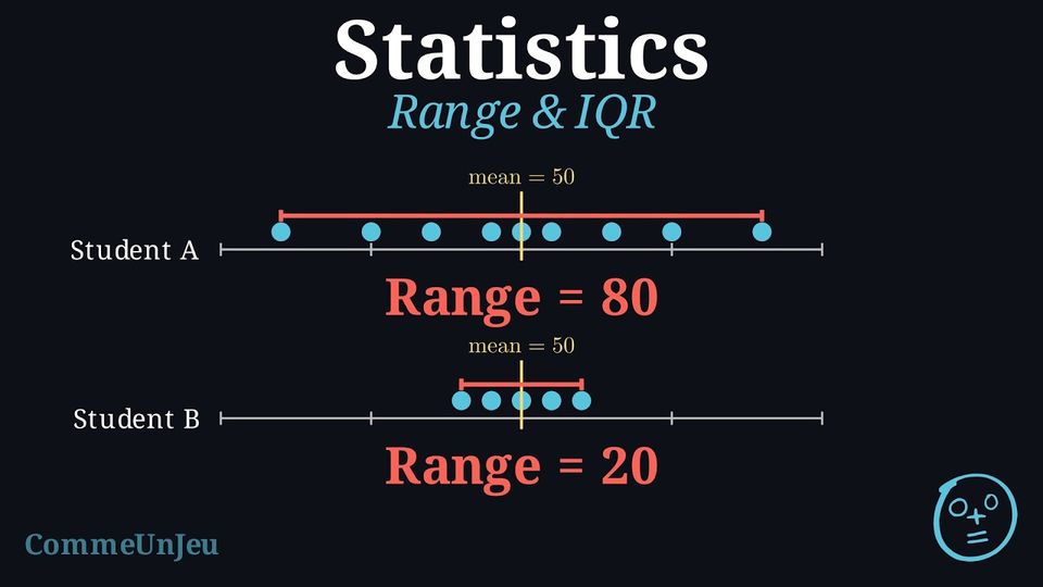
Definition — Range
The range is the difference between the maximum and minimum values in a dataset. It gives a quick measure of the total spread. $$ \text{Range} = \text{Maximum Value} - \text{Minimum Value} $$ Definition — Quartiles and IQR
Quartiles are values that divide an ordered dataset into four parts, each holding about a quarter of the values. - The lower quartile (Q1) is the median of the lower half of the data.
- The median (Q2) is the overall median of the data.
- The upper quartile (Q3) is the median of the upper half of the data.
The interquartile range (IQR) is the range of the middle 50\(\pourcent\) of the data. It is less affected by extreme outliers than the range. $$ \text{IQR} = Q_3 - Q_1 $$
Example
Find the quartiles and the interquartile range for the data: \(1, 19, 10, 2, 18, 10, 5, 15, 10\). - Order the data: \(1, 2, 5, 10, 10, 10, 15, 18, 19\).
- Find the median (Q2): The middle value is the 5th one, so \(Q_2 = 10\). $$ 1, 2, 5, 10, \underline{10}, 10, 15, 18, 19 $$
- Split the data into two halves (excluding Q2): Lower half: \(1, 2, 5, 10\) \(\quad\) Upper half: \(10, 15, 18, 19\).
- Find the lower quartile (Q1): Find the median of the lower half. $$ 1, \underline{2, 5}, 10 \rightarrow Q_1 = \frac{2+5}{2} = 3.5 $$
- Find the upper quartile (Q3): Find the median of the upper half. $$ 10, \underline{15, 18}, 19 \rightarrow Q_3 = \frac{15+18}{2} = 16.5 $$
- Calculate the IQR: $$ \text{IQR} = Q_3 - Q_1 = 16.5 - 3.5 = 13 $$
Two Conventions for Quartiles
Two conventions coexist for quartiles. In one convention, the quartiles are the medians of the two halves of the dataset (they may fall between two values). In the other, used in the following definition, the quartiles are always values of the dataset. The two conventions can give different numbers on the same dataset — what matters is to state which convention is used.
Definition — Quartiles as Values of the Dataset
For an ordered dataset of \(N\) values: - the first quartile \(Q_1\) is the smallest value of the dataset such that at least one quarter (\(25\pourcent\)) of the values are less than or equal to it;
- the third quartile \(Q_3\) is the smallest value of the dataset such that at least three quarters (\(75\pourcent\)) of the values are less than or equal to it.
Skills to practice
- Finding the Interquartile Range
II.2
Variance and Standard Deviation
Recappreviously studied — click to reread
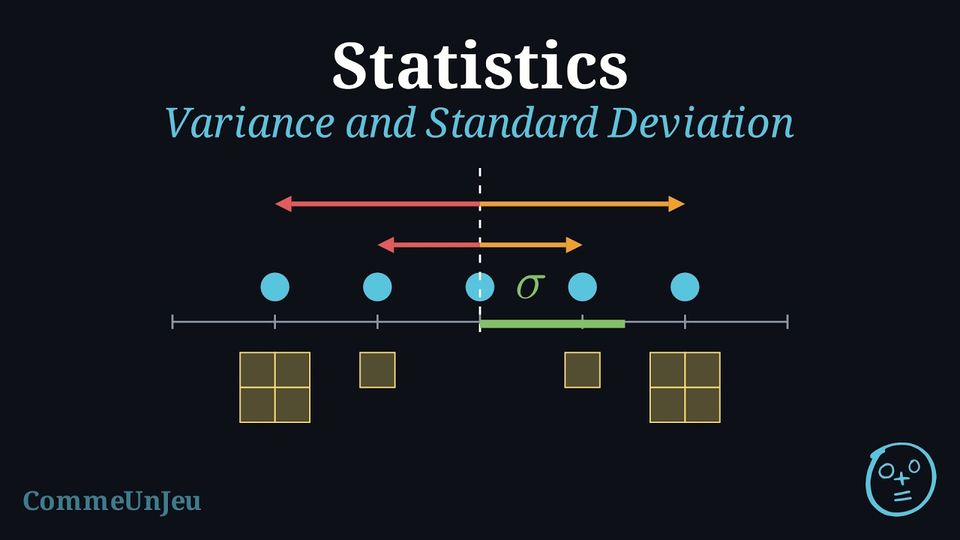
Definition — Variance and Standard Deviation
The variance \(V\) of a data set measures the average of the squared distances of the values from the mean \(\bar{x}\). When the values \(x_i\) have frequencies \(n_i\) (with \(N = \sum n_i\)): $$ V = \frac{1}{N}\sum_{i=1}^{k} n_i (x_i - \bar{x})^2 . $$ The standard deviation \(\sigma\) is the square root of the variance: $$ \sigma = \sqrt{V} = \sqrt{\frac{1}{N}\sum_{i=1}^{k} n_i (x_i - \bar{x})^2} . $$ The variance is expressed in the squared unit of the data, whereas the standard deviation is back in the original unit, which makes it the natural measure of typical distance to the mean. This is the population (descriptive) variance, with denominator \(N\).
The standard deviation is above all a comparison instrument. Two data sets can share the same mean yet differ greatly in how the values are scattered around it: the set with the smaller standard deviation is the more consistent (regular) one. For example, a striker who scores \(\{2,3,4,5,6\}\) goals across five matches and one who scores \(\{3,4,4,4,5\}\) both average \(4\) goals; their variances are \(2\) and \(0.4\) respectively, so the second striker is far more consistent — the same average hides very different regularity.
Example
During \(10\) matches, a player scored the numbers of goals given in the frequency table below. Compute the variance \(V\) and the standard deviation \(\sigma\) of the number of goals. | Goals \(x_i\) | 0 | 1 | 2 | 3 | Total |
| Frequency \(n_i\) | 3 | 4 | 2 | 1 | 10 |
Step 1 — Mean. With \(N = 3+4+2+1 = 10\) and \(\sum n_i x_i = 0\cdot 3 + 1\cdot 4 + 2\cdot 2 + 3\cdot 1 = 11\): $$ \bar{x} = \frac{11}{10} = 1.1 . $$ Step 2 — Squared deviations weighted by frequency.
Step 3 — Variance, then standard deviation. $$ \begin{aligned} V &= \frac{1}{N}\sum n_i (x_i-\bar{x})^2 &&\text{(definition)} \\
&= \frac{8.90}{10} &&\text{(substitute)} \\
&= 0.89 ; &&\text{(divide)} \\
\sigma &= \sqrt{V} = \sqrt{0.89} &&\text{(square root)} \\
&\approx 0.94 . &&\text{(evaluate)} \end{aligned} $$ The variance is \(0.89\) goal\(^2\) and the standard deviation is about \(0.94\) goal.
| \(x_i\) | \(n_i\) | \(x_i-\bar{x}\) | \((x_i-\bar{x})^2\) | \(n_i(x_i-\bar{x})^2\) |
| 0 | 3 | \(-1.1\) | \(1.21\) | \(3.63\) |
| 1 | 4 | \(-0.1\) | \(0.01\) | \(0.04\) |
| 2 | 2 | \(0.9\) | \(0.81\) | \(1.62\) |
| 3 | 1 | \(1.9\) | \(3.61\) | \(3.61\) |
| Total | 10 | 8.90 |
The variance defined here divides by \(N\): it describes the data set itself (the population variance). When the data set is only a sample drawn to estimate a larger population, statistical software and calculators offer a second variance, the sample variance, which divides by \(N-1\) instead of \(N\). Dividing by the slightly smaller \(N-1\) gives a slightly larger value that better estimates the spread of the whole population. The two coincide for large \(N\); the population version (denominator \(N\)) is the one used.
Skills to practice
- Calculating the Standard Deviation
III
Box Plots and the Shape of a Distribution
III.1
Box Plots
Recappreviously studied — click to reread
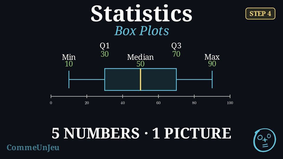
Definition — Box Plot
A box plot visually displays the five-number summary above a number line. - A central box is drawn from the lower quartile (Q1) to the upper quartile (Q3).
- A line inside the box marks the median (Q2).
- Whiskers (lines) extend from the box out to the minimum and maximum values.

Method — Constructing a Box Plot
- Order the data from least to greatest.
- Find the five-number summary: Calculate the minimum, Q1, median, Q3, and maximum.
- Draw a number line that covers the full range of your data.
- Draw the box and median: Draw a box from Q1 to Q3 and a vertical line inside the box at the median.
- Draw the whiskers: Draw lines from the box to the minimum and maximum values.
Method — Choosing the Measures to Compare
To compare two datasets, pair a measure of centre with its measure of spread: - the mean \(\bar{x}\) goes with the standard deviation \(\sigma\) — they use every value, but extreme values pull them;
- the median goes with the interquartile range — they are read off positions in the ordered list, so one extreme value barely moves them.
Skills to practice
- Reading and Comparing Box Plots
III.2
Outliers
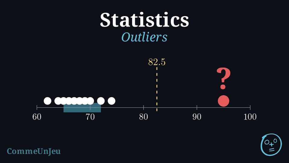
The eleven members of an athletics club ran a \(400\) m race. Their times, in seconds and in increasing order, are: $$62,\ 64,\ 65,\ 66,\ 67,\ 68,\ 69,\ 70,\ 72,\ 74,\ 95.$$ The time \(95\) s stands apart from the others.
Is \(95\) s an unusual time for this club, or simply the slowest one? And \(74\) s? Two people looking at the list may disagree: what yardstick could a rule use, so that everyone decides the same way?
Is \(95\) s an unusual time for this club, or simply the slowest one? And \(74\) s? Two people looking at the list may disagree: what yardstick could a rule use, so that everyone decides the same way?
The yardstick is the width of the central half of the data: the interquartile range. With \(N = 11\) times, the median is the \(6^{\text{th}}\) ordered value, \(68\). The lower half \(62, \ldots, 67\) and the upper half \(69, \ldots, 95\) hold five values each, and their medians are \(Q_1 = 65\) and \(Q_3 = 72\) (the convention of quartiles as values of the dataset gives the same values), so \(\text{IQR} = 72 - 65 = 7\). The usual rule looks one and a half interquartile ranges beyond each quartile: $$\begin{aligned}[t] Q_3 + 1.5 \times \text{IQR} &= 72 + 1.5 \times 7 && \text{(}1.5\text{ IQR above } Q_3\text{)}\\
&= 72 + 10.5\\
&= 82.5, \\
Q_1 - 1.5 \times \text{IQR} &= 65 - 10.5 && \text{(}1.5\text{ IQR below } Q_1\text{)}\\
&= 54.5. \end{aligned}$$ The time \(95\) s lies beyond \(82.5\) s: it is unusual for this club, an outlier. The time \(74\) s lies below \(82.5\) s: it is simply the second slowest time. No time lies below \(54.5\) s.
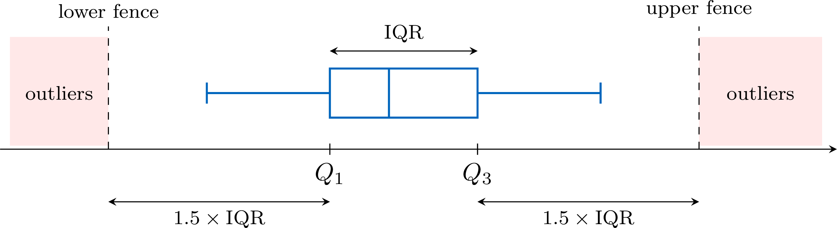
Definition — Fences and Outliers
Consider a dataset with lower quartile \(Q_1\), upper quartile \(Q_3\) and interquartile range \(\text{IQR} = Q_3 - Q_1\). - The lower fence is \(Q_1 - 1.5 \times \text{IQR}\).
- The upper fence is \(Q_3 + 1.5 \times \text{IQR}\).
Method — Testing Data for Outliers
- Find the quartiles: order the data, then find \(Q_1\) and \(Q_3\) as the medians of the two halves (the median left out when the number of values is odd).
- Compute the yardstick: \(\text{IQR} = Q_3 - Q_1\), then \(1.5 \times \text{IQR}\).
- Compute the two fences: \(Q_1 - 1.5 \times \text{IQR}\) and \(Q_3 + 1.5 \times \text{IQR}\).
- Compare the extreme values with the fences: the smallest values with the lower fence, the largest ones with the upper fence. Every value strictly beyond a fence is an outlier; a value equal to a fence is not.
- Interpret in context: a recording error is corrected, or removed if the true value is unknown; a genuine value is kept and reported.
Example
Over \(15\) working days, a small office recorded the number of emails it received each day. In increasing order: $$12,\ 18,\ 19,\ 21,\ 22,\ 23,\ 24,\ 25,\ 26,\ 27,\ 28,\ 30,\ 31,\ 33,\ 48.$$ Test these data for outliers.
Quartiles. With \(N = 15\) values, the median is the \(8^{\text{th}}\) ordered value, \(25\). The two halves, \(12, \ldots, 24\) and \(26, \ldots, 48\), hold seven values each, and their medians are their \(4^{\text{th}}\) values: \(Q_1 = 21\) and \(Q_3 = 30\) (the convention of quartiles as values of the dataset gives the same values).
Yardstick. \(\text{IQR} = Q_3 - Q_1 = 30 - 21 = 9\), so \(1.5 \times \text{IQR} = 1.5 \times 9 = 13.5\).
Fences. $$\begin{aligned}[t] \text{lower fence} &= Q_1 - 1.5 \times \text{IQR} && \text{(definition)}\\ &= 21 - 13.5 && \text{(}Q_1 = 21\text{)}\\ &= 7.5,\\ \text{upper fence} &= Q_3 + 1.5 \times \text{IQR} && \text{(definition)}\\ &= 30 + 13.5 && \text{(}Q_3 = 30\text{)}\\ &= 43.5. \end{aligned}$$ Comparison. The smallest value, \(12\), is above \(7.5\): there is no outlier on the low side, even though \(12\) is well below the other values. The largest value, \(48\), is above \(43.5\): it is an outlier; the next one, \(33\), is not.
Conclusion. The only outlier is the day with \(48\) emails. It is a day to look into (a mailing campaign, a failure of the mail server the day before), not a value to delete automatically.
Method — Drawing a Box Plot with Outliers
When a dataset has outliers, its box plot shows them apart from the other values. - Draw the box and the median line from \(Q_1\) to \(Q_3\), as usual.
- Stop each whisker at the most extreme value that is not an outlier.
- Mark each outlier with a cross \(\times\) at its value.
Example
The numbers of emails received by an office over \(15\) working days are, in increasing order: $$12,\ 18,\ 19,\ 21,\ 22,\ 23,\ 24,\ 25,\ 26,\ 27,\ 28,\ 30,\ 31,\ 33,\ 48.$$ Their quartiles are \(Q_1 = 21\) and \(Q_3 = 30\), and their only outlier is \(48\). Draw their box plot, with the outlier marked.
The median is the \(8^{\text{th}}\) of the \(15\) ordered values: \(25\). The box runs from \(Q_1 = 21\) to \(Q_3 = 30\), with the median line at \(25\). The left whisker goes down to \(12\), which is not an outlier. The right whisker stops at \(33\), the largest value that is not an outlier, and \(48\) is marked by a cross. 
Drawn to \(48\), the right whisker would hide the gap between \(33\) and \(48\): nothing on the plot would show that \(48\) stands apart from the other values.
What to Do with an Outlier
An outlier is first checked. A recording error — a height of \(1\,720\) cm typed instead of \(172\) cm — is corrected, or removed if the true value is unknown. A genuine value — the record day of a shop — is kept: it is part of the data, and often the most interesting part of it. The size of an outlier pulls the mean, but plays no part in the median and the interquartile range, which depend on the middle values of the ordered list: when there are outliers, the pair median–IQR describes the data better. Finally, the factor \(1.5\) is a convention designed for roughly symmetric data: in a distribution with a long tail on one side, the rule flags several values of that tail, which are rare but normal for such a shape.
Skills to practice
- Testing Values for Outliers
- Testing for Outliers and Drawing the Box Plot
III.3
Shape of a Distribution
A library recorded how long each of its \(40\) visitors stayed one afternoon, in minutes. The histogram shows the durations, grouped in classes of \(20\) minutes. 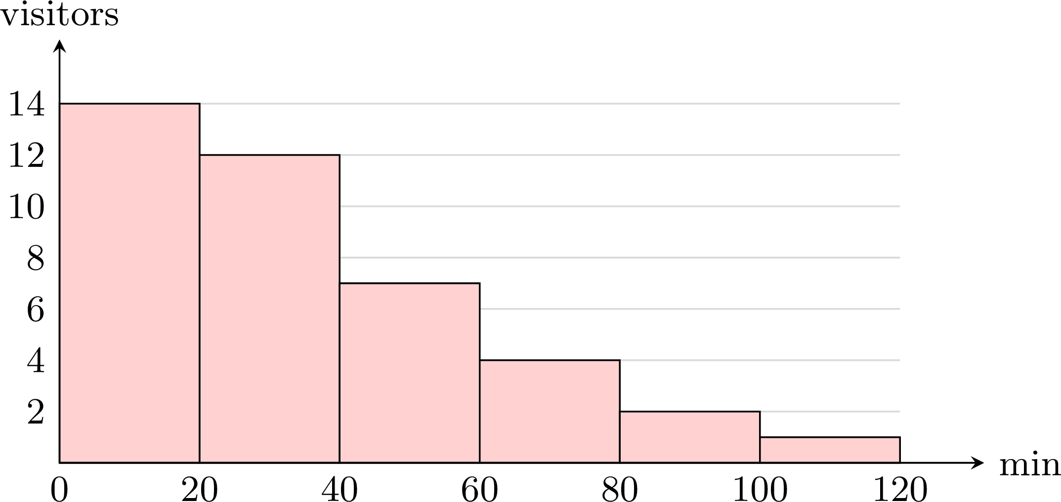
Where are most of the durations? On which side does the histogram stretch out?
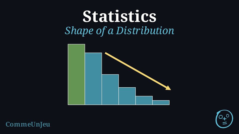
Most visits are short: \(14 + 12 = 26\) of the \(40\) visits last less than \(40\) minutes. Then the bars get shorter and shorter towards the long visits, up to the class from \(100\) to \(120\) minutes. The histogram stretches out on the right, in a long tail of rare, long visits: such a distribution is said to be skewed to the right.
Definition — Shape of a Distribution
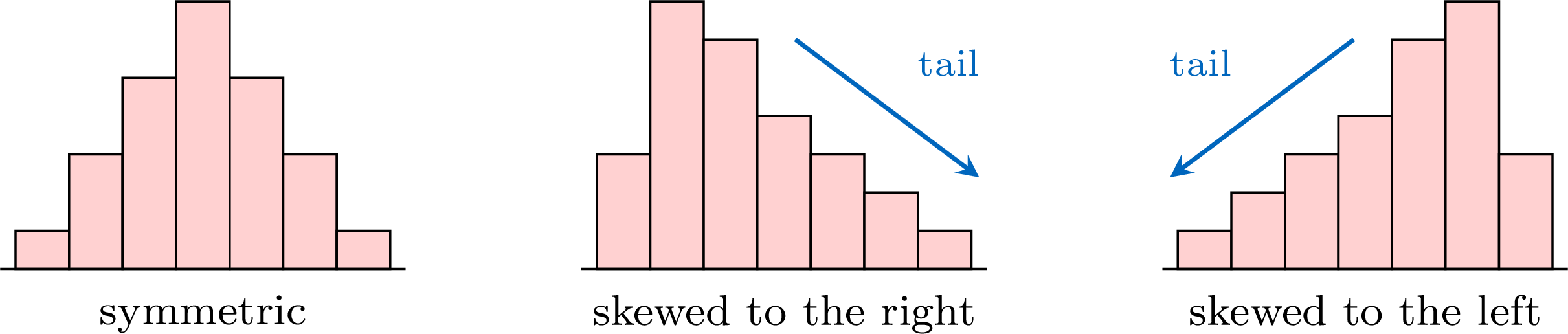
The distribution of a dataset is the way its values are spread along the axis, as a histogram or a bar chart shows it. Its shape is described by comparing its two sides. - The distribution is symmetric when its two sides, on either side of the middle, are roughly mirror images of each other.
- It is skewed to the right (or positively skewed) when its graph has a long tail stretching towards the large values.
- It is skewed to the left (or negatively skewed) when its long tail stretches towards the small values.
Method — Reading the Shape on a Box Plot
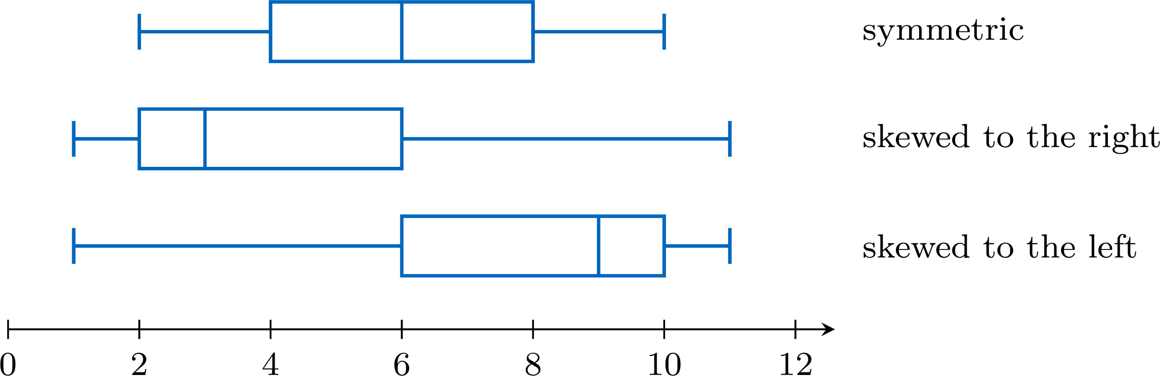
A box plot cuts the ordered data into four parts, each holding about a quarter of the values (when outliers are marked, they belong to the outer quarters, beyond the whiskers). Compare the two halves of the box (from \(Q_1\) to the median, from the median to \(Q_3\)) and the two whiskers. - Symmetric: the median is near the middle of the box, and the two whiskers have about the same length.
- Skewed to the right: the right half of the box and the right whisker are the longer ones — the median is closer to \(Q_1\).
- Skewed to the left: the left half of the box and the left whisker are the longer ones — the median is closer to \(Q_3\).
Example
The box plot shows the times, in minutes, that \(40\) pupils took to solve a puzzle. Describe the shape of the distribution. 
The five-number summary read on the plot is: minimum \(2\), \(Q_1 = 4\), median \(5\), \(Q_3 = 9\), maximum \(16\). The lengths of the four parts are:
The right half of the box is four times as long as the left half, and the right whisker is longer than the left one: the distribution is skewed to the right. In context: the quarter of the pupils just below the median are packed between \(4\) and \(5\) minutes, whereas the slow times are spread out, up to \(16\) minutes.
| left whisker | left half of the box | right half of the box | right whisker |
| \(4 - 2 = 2\) | \(5 - 4 = 1\) | \(9 - 5 = 4\) | \(16 - 9 = 7\) |
Method — Comparing the Mean and the Median
The mean uses the size of every value, whereas the median only depends on the value or values in the middle of the ordered list. A long tail therefore pulls the mean towards it, while the size of its values plays no part in the median. - Mean close to the median: consistent with a symmetric distribution.
- Mean clearly greater than the median: the sign of a long tail on the right, that is of a distribution skewed to the right.
- Mean clearly smaller than the median: the sign of a distribution skewed to the left.
Example
Eleven pupils noted how many minutes they spent on their phone one evening, in increasing order: $$15,\ 20,\ 25,\ 25,\ 30,\ 30,\ 35,\ 40,\ 45,\ 60,\ 115.$$ - Compute the mean and the median.
- What does their comparison suggest about the shape of the distribution?
- The value \(115\) is removed. Compute the new mean and the new median.
- The mean is $$\begin{aligned}[t] \bar{x} &= \frac{15 + 20 + 25 + 25 + 30 + 30 + 35 + 40 + 45 + 60 + 115}{11} && \text{(definition of the mean)}\\ &= \frac{440}{11} && \text{(sum of the values)}\\ &= 40. \end{aligned}$$ There are \(11\) ordered values: the median is the \(6^{\text{th}}\) one, \(30\).
- The mean (\(40\) minutes) is clearly greater than the median (\(30\) minutes): this suggests a distribution skewed to the right. The list confirms it: the values climb slowly up to \(45\), then jump to \(60\) and \(115\) — a long tail on the right. (With \(Q_1 = 25\) and \(Q_3 = 45\), the upper fence is \(45 + 1.5 \times 20 = 75\): the value \(115\) is even an outlier.)
- Without \(115\), the sum is \(440 - 115 = 325\) for \(10\) values, so the new mean is \(\frac{325}{10} = 32.5\). The new median is the mean of the \(5^{\text{th}}\) and \(6^{\text{th}}\) of the \(10\) values: \(\frac{30 + 30}{2} = 30\). Removing one value of the tail lowered the mean by \(7.5\) minutes and left the median unchanged.
Symmetric Does Not Mean Normal
Many measurements — the heights of adults, the masses of the apples of one orchard, the errors of a measuring instrument — have a bell-shaped distribution: a single peak in the middle, a symmetric shape, and frequencies that decrease steadily on both sides. The model of such data is called the normal distribution.
A normal distribution has a symmetric box plot, and data drawn from it usually give a nearly symmetric one. The converse is false: a symmetric box plot is consistent with a normal distribution, but it never proves it. The three datasets below all have a symmetric box plot; only the first one is bell-shaped. 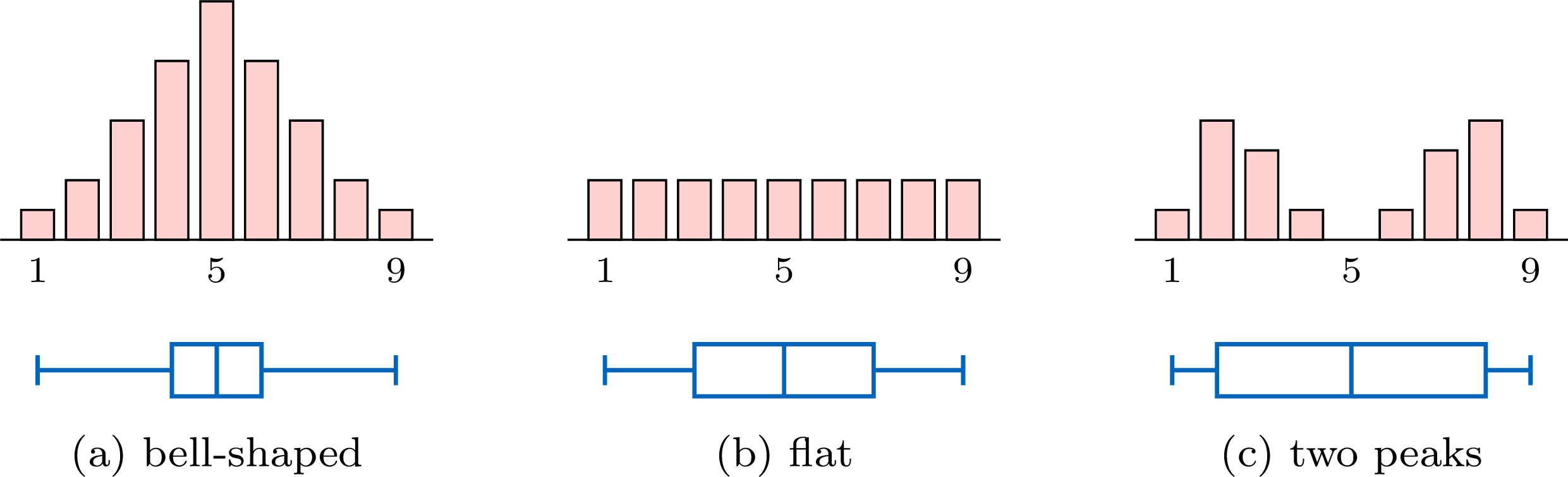
Their five-number summaries are \(1, 4, 5, 6, 9\) for (a), \(1, 3, 5, 7, 9\) for (b) and \(1, 2, 5, 8, 9\) for (c): each box plot is symmetric about the median \(5\). A box plot keeps only five numbers. To judge whether data may come from a normal distribution, look at the histogram as well: a single peak, in the middle, and frequencies that decrease on both sides.
A normal distribution has a symmetric box plot, and data drawn from it usually give a nearly symmetric one. The converse is false: a symmetric box plot is consistent with a normal distribution, but it never proves it. The three datasets below all have a symmetric box plot; only the first one is bell-shaped.
Skills to practice
- Recognising the Shape of a Distribution
- Justifying the Shape of a Distribution
IV
Grouped Data and Cumulative Frequency
IV.1
Grouped Data
Recappreviously studied — click to reread
Method — Estimating the Mean of Grouped Data
The exact values inside a class are unknown, so the mean is estimated by representing each class by its midpoint (the centre of the interval). - Find each class midpoint \(m_i\): the average of the two endpoints of the class.
- Multiply each midpoint by the class frequency \(n_i\) to get \(n_i m_i\).
- Estimate the mean as a weighted mean of the midpoints: $$ \bar{x} \approx \frac{\sum n_i m_i}{N}, \qquad N = \sum n_i . $$
Example
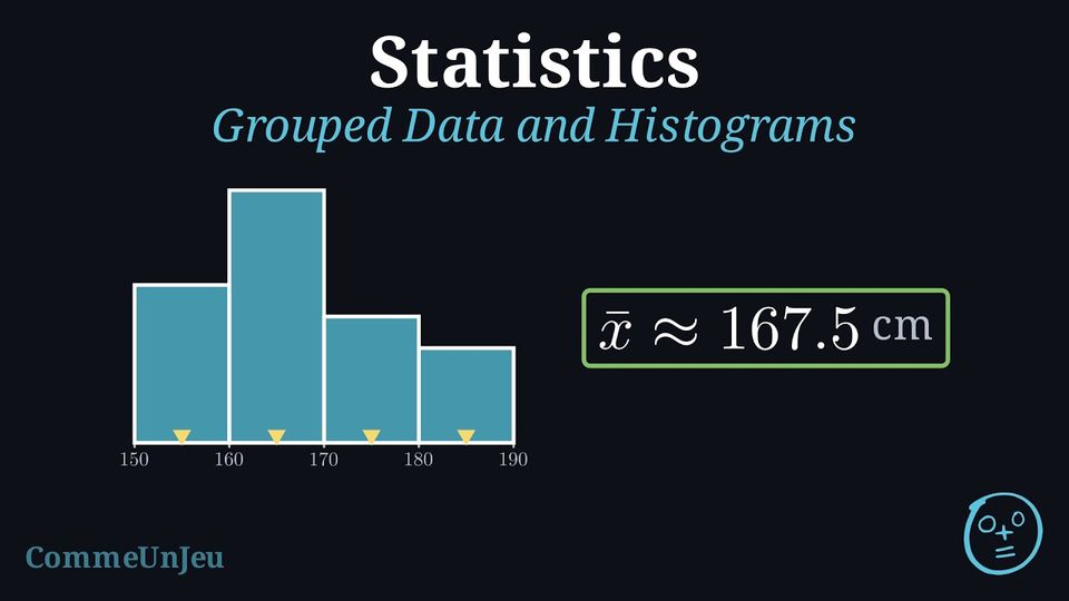
The heights (in cm) of \(20\) students were measured and grouped into classes. Draw the histogram and estimate the mean height. | Height (cm) | \([150,160)\) | \([160,170)\) | \([170,180)\) | \([180,190)\) | Total |
| Frequency \(n_i\) | 5 | 8 | 4 | 3 | 20 |
Histogram. The bars are adjacent (no gaps), since the classes are consecutive intervals. 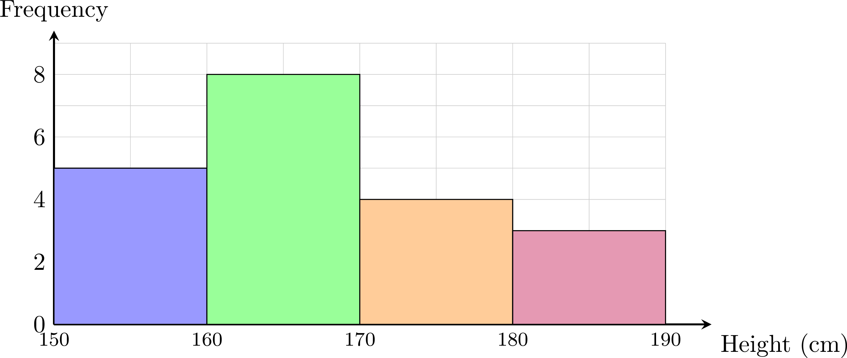
Estimated mean. The midpoints are \(m_i = 155, 165, 175, 185\).
$$ \begin{aligned} \bar{x} &\approx \frac{\sum n_i m_i}{N} &&\text{(midpoint estimate)} \\
&= \frac{155\times 5 + 165\times 8 + 175\times 4 + 185\times 3}{20} &&\text{(substitute)} \\
&= \frac{3350}{20} &&\text{(add)} \\
&= 167.5 . &&\text{(divide)} \end{aligned} $$ The estimated mean height is about \(167.5\) cm.
| Class | \([150,160)\) | \([160,170)\) | \([170,180)\) | \([180,190)\) | Total |
| Midpoint \(m_i\) | 155 | 165 | 175 | 185 | |
| \(n_i\) | 5 | 8 | 4 | 3 | 20 |
| \(n_i m_i\) | 775 | 1320 | 700 | 555 | 3350 |
Proposition — Mean from the Class Means
A series of \(N\) values is sorted into \(k\) classes of frequencies \(n_1, n_2, \ldots, n_k\), and the mean of the values of each class is known: \(\bar{x}_1, \bar{x}_2, \ldots, \bar{x}_k\). The mean of the whole series is the weighted mean of the class means, each mean weighted by the frequency of its class: $$\textcolor{colorprop}{\bar{x} = \frac{n_1 \bar{x}_1 + n_2 \bar{x}_2 + \cdots + n_k \bar{x}_k}{N}}, \qquad N = n_1 + n_2 + \cdots + n_k.$$ Special case: when the values of a class are assumed to be spread uniformly between its bounds — the model behind the midpoint estimate — the mean of the class is taken to be its midpoint, and the formula gives the estimate of the mean by the midpoints.
By the definition of the mean, the sum of the \(n_i\) values of the class number \(i\) is \(n_i \bar{x}_i\). The sum of all \(N\) values is the sum of these class sums, so $$\begin{aligned} \bar{x} &= \frac{\text{sum of the } N \text{ values}}{N} && \text{(definition of the mean)} \\
&= \frac{n_1 \bar{x}_1 + n_2 \bar{x}_2 + \cdots + n_k \bar{x}_k}{N}. && \text{(sum class by class)} \end{aligned}$$ When the values of a class are modelled as spread uniformly between its two bounds, they are balanced around the midpoint of the class, which is then taken as the mean of the class: the formula becomes the midpoint estimate.
Skills to practice
- Estimating the Mean of Grouped Data
IV.2
Cumulative Frequency
Recappreviously studied — click to reread
Definition — Cumulative Frequency
The cumulative frequency of a value (or of the upper end of a class) is the running total of all frequencies up to and including that value. Reading the table from top to bottom, each cumulative frequency adds the next frequency to the previous total, so the last cumulative frequency equals the total number of data values \(N\). Definition — Cumulative-Frequency Curve (Ogive)
When data is grouped into classes, the running totals can be displayed graphically as the cumulative-frequency curve (or ogive). It is built by plotting each cumulative frequency against the upper boundary of its class and joining the points in order by straight segments, starting from the lower boundary of the first class at height \(0\). The curve never goes down: it climbs from \(0\) to the total \(N\), and the number of values below any level can be estimated from it. In particular, the median is estimated by reading across from the height \(\dfrac{N}{2}\) on the vertical axis to the curve, then down to the horizontal axis. In the same way, the lower quartile \(Q_1\) and the upper quartile \(Q_3\) are estimated by reading across from the heights \(\dfrac{N}{4}\) and \(\dfrac{3N}{4}\), which gives an estimate of the interquartile range \(Q_3 - Q_1\). Method — Finding the Median from Cumulative Frequencies
- Compute the cumulative frequencies by running totals.
- Locate the middle position(s): position \(\dfrac{N+1}{2}\) if \(N\) is odd; the two positions \(\dfrac{N}{2}\) and \(\dfrac{N}{2}+1\) if \(N\) is even.
- Read off the median: the cumulative frequencies tell which value occupies each ordered position. For odd \(N\), it is the value at the middle position; for even \(N\), the average of the values at the two middle positions (often the same value).
Example
The table gives the test scores (out of \(100\)) of \(50\) students, grouped into classes. Draw the cumulative-frequency curve and use it to estimate the median score. | Score | \([0,20)\) | \([20,40)\) | \([40,60)\) | \([60,80)\) | \([80,100)\) | Total |
| Frequency \(n_i\) | 5 | 10 | 20 | 10 | 5 | 50 |
Form the cumulative frequencies, taking each one at the upper boundary of its class:
Plotting these points (with \((0,0)\)) and joining them gives the ogive: 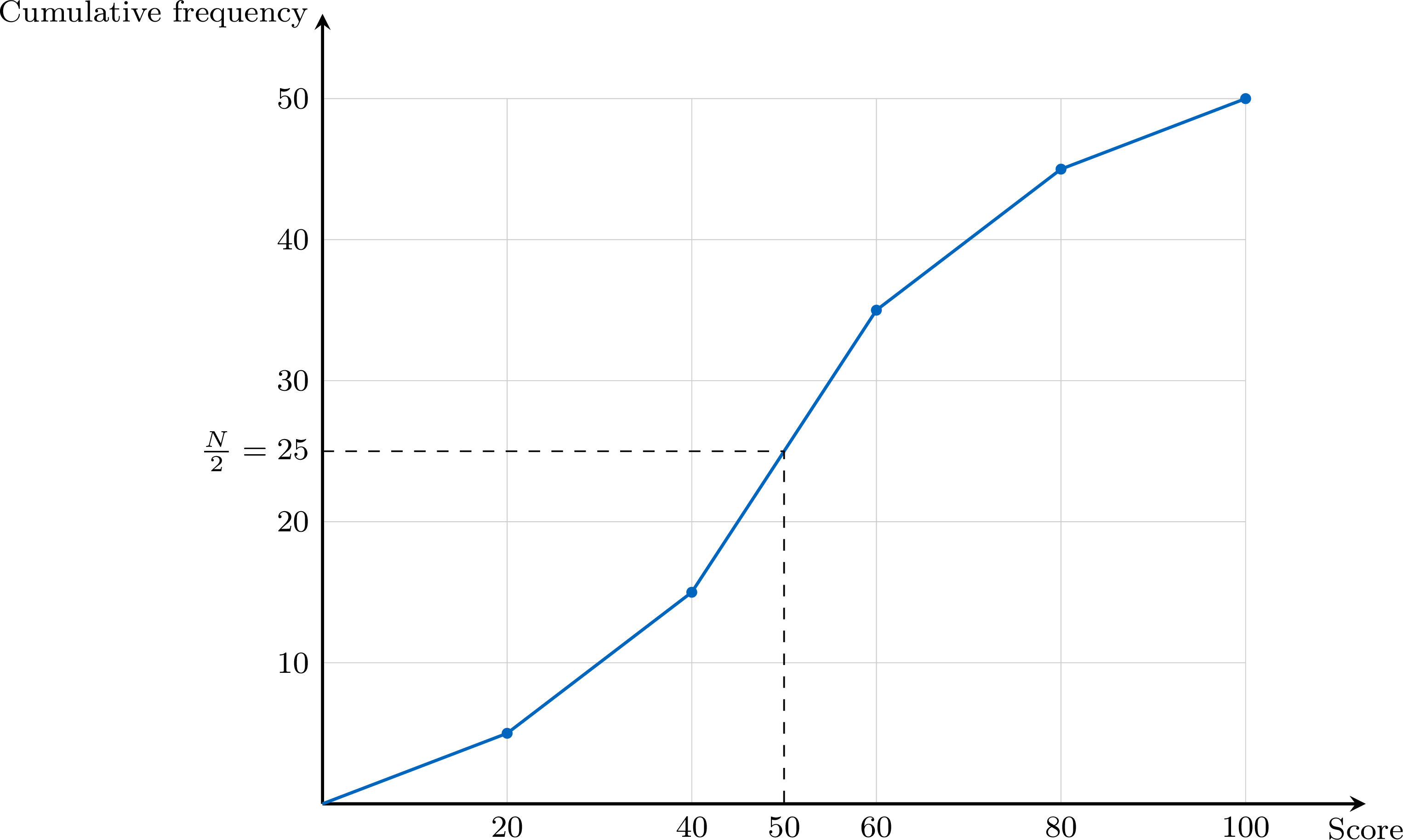
With \(N = 50\), read across from \(\dfrac{N}{2} = 25\) to the curve and down to the axis: the curve reaches this height at a score of about \(50\), so $$ \text{median} \approx 50 \text{ marks.} $$
| Upper boundary | 20 | 40 | 60 | 80 | 100 |
| Cumulative frequency | 5 | 15 | 35 | 45 | 50 |
Definition — Median Class
For a series of \(N\) values grouped into classes, the median class is the class where the median is located: reading the cumulative frequencies in order, it is the first class whose cumulative frequency reaches or exceeds \(\dfrac{N}{2}\). Equivalently, it is the first class whose cumulative relative frequency reaches or exceeds \(50\pourcent\). If a cumulative frequency is exactly \(\dfrac{N}{2}\), the middle of the series falls on the boundary between that class and the next one, and the estimate below returns that boundary. Method — Estimating the Median by a Uniform Spread in the Median Class
The exact values inside the median class are unknown. Assuming that its \(n_c\) values are spread uniformly between its bounds \(a\) and \(b\): - Compute the cumulative frequencies and find the median class \([a, b)\); write \(n_{\text{before}}\) for the cumulative frequency of the classes before it.
- Count the values needed inside the median class to reach the middle: \(\dfrac{N}{2} - n_{\text{before}}\), out of the \(n_c\) values of the class.
- Move along the class in the same proportion: $$\text{median} \approx a + \frac{\dfrac{N}{2} - n_{\text{before}}}{n_c} \times (b - a).$$
Cumulative Frequency Polygon
Dividing each cumulative frequency by \(N\) gives the cumulative relative frequencies, which run from \(0\) to \(1\), that is from \(0\pourcent\) to \(100\pourcent\). Plotted against the upper bounds of the classes and joined by segments from the lower bound of the first class, they form the cumulative frequency polygon: the same broken line as the cumulative-frequency curve, with a vertical axis in percentages. An estimate of the median is read at the height \(50\pourcent\); the proportion of the values below a class boundary is read directly on the vertical axis, and between two boundaries the polygon gives an estimate of it, whatever the size \(N\) of the series — which makes the polygon the right tool to compare two series of different sizes.
Skills to practice
- Finding the Median from Cumulative Frequencies
IV.3
Percentiles
Definition — Percentile
Let \(k\) be a whole number from \(1\) to \(99\). A \(k\)-th percentile \(P_k\) of a dataset is a value such that at least \(k\pourcent\) of the values are less than or equal to \(P_k\), and at least \((100 - k)\pourcent\) are greater than or equal to \(P_k\): roughly, \(k\pourcent\) of the data are less than or equal to \(P_k\). For raw data several values may fit, and a convention chooses one, as for the quartiles. For data grouped in classes, \(P_k\) is estimated on the cumulative frequency graph: it is the value at which the cumulative frequency reaches \(k\pourcent\) of the total.On a cumulative frequency graph, the quartiles are read as the percentiles of orders \(25\), \(50\) and \(75\): \(Q_1 = P_{25}\), the median is \(P_{50}\) and \(Q_3 = P_{75}\). For raw data, the quartiles taken as values of the dataset are percentiles in this sense, whereas the medians of the two halves can differ slightly from them. The percentiles \(P_{10}\) and \(P_{90}\) are also called the first and the ninth deciles.
Method — Reading Percentiles on a Cumulative Frequency Graph
On the cumulative frequency graph of a dataset of \(N\) values: - Compute the height \(\dfrac{k}{100} \times N\), or read \(k\pourcent\) directly on a percentage scale.
- Read across from this height on the vertical axis to the graph.
- Read down to the horizontal axis: the value read is \(P_k\).
Example
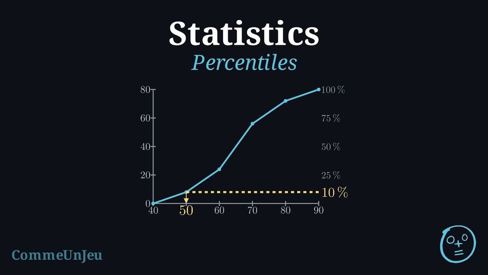
The times of the \(80\) runners of a \(10\) km race are grouped in classes of \(10\) minutes. | Time (min) | \([40, 50)\) | \([50, 60)\) | \([60, 70)\) | \([70, 80)\) | \([80, 90)\) |
| Runners | \(8\) | \(16\) | \(32\) | \(16\) | \(8\) |
- Estimate the quartiles and the interquartile range of the times.
- The fastest \(10\pourcent\) of the runners receive a medal. Which time did they beat?
- What percentage of the runners finished in less than \(70\) minutes? How many runners took more than \(75\) minutes?
The cumulative frequencies, taken at the upper bounds \(50, 60, 70, 80, 90\), are \(8, 24, 56, 72, 80\); the polygon starts at \((40, 0)\). The right-hand scale gives the percentages of the \(80\) runners. 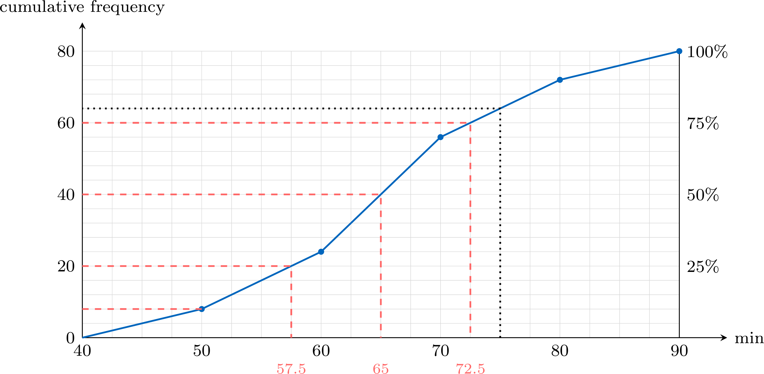
- \(Q_1 = P_{25}\) is read at the height \(\frac{25}{100} \times 80 = 20\), the median at \(40\) and \(Q_3\) at \(60\). The reading gives the estimates \(Q_1 \approx 57.5\), median \(\approx 65\) and \(Q_3 \approx 72.5\) minutes. On the polygon each reading can be computed by proportion; for \(Q_1\), the height \(20\) lies in the class \([50, 60)\), between the cumulative frequencies \(8\) and \(24\): $$Q_1 \approx 50 + \frac{20 - 8}{24 - 8} \times 10 = 50 + 7.5 = 57.5.$$ The interquartile range is about \(\text{IQR} = 72.5 - 57.5 = 15\) minutes.
- The fastest runners are those with the smallest times: the fastest \(10\pourcent\) are below \(P_{10}\). The height \(\frac{10}{100} \times 80 = 8\) is reached at \(50\) minutes, a class boundary: exactly \(8\) runners, the medal winners, finished in less than \(50\) minutes.
- Up from \(70\) minutes, a class boundary, the cumulative frequency is \(56\): \(\frac{56}{80} = 70\pourcent\) of the runners finished in less than \(70\) minutes. Up from \(75\) minutes (dotted line), the polygon gives \(64\): an estimated \(80 - 64 = 16\) runners took more than \(75\) minutes — an estimate, since \(75\) lies inside the class \([70, 80)\).
A Percentile Is Not a Percentage of the Marks
Being at the \(90\)th percentile of a test means that about \(90\pourcent\) of the candidates scored at most the same mark — not that the mark is \(90\pourcent\) of the maximum. On a hard test, a mark of \(12\) out of \(20\) can be the \(90\)th percentile; on an easy one, \(17\) out of \(20\) can be the median. And when the best results are the smallest values, as for times, the best \(10\pourcent\) lie below \(P_{10}\), not above \(P_{90}\).
Skills to practice
- Reading Percentiles on a Cumulative Frequency Graph
- Interpreting Percentiles in Context
IV.4
The Modal Class
Definition — Modal Class
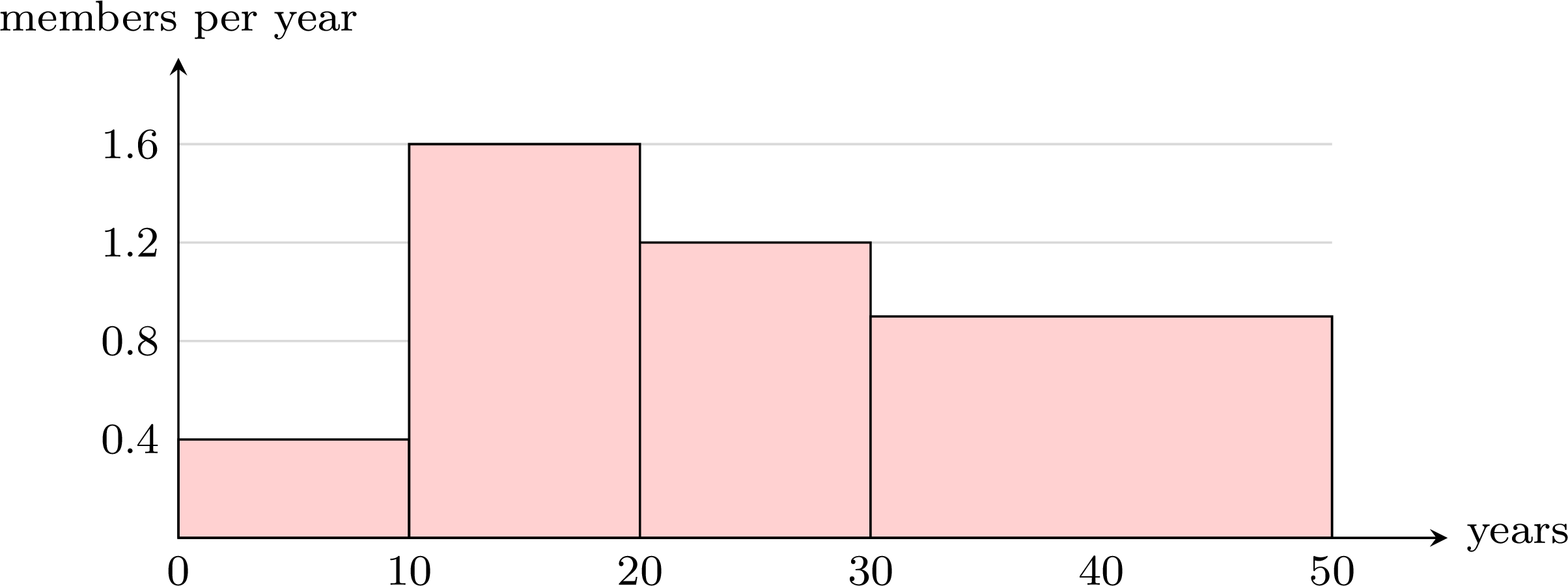
For data grouped into classes of the same width, the modal class is the class with the highest frequency: the class of the tallest bar of the histogram. When the classes have different widths, the modal class is still the class of the tallest bar, whose height is the frequency divided by the width of the class — the frequency per unit of width.The modal class shows where the values are the most concentrated. It can differ from the median class, which contains the middle of the ordered data.
Example
The ages of the \(50\) members of a sailing club are grouped in classes of \(10\) years. | Age (years) | \([0, 10)\) | \([10, 20)\) | \([20, 30)\) | \([30, 40)\) | \([40, 50)\) |
| Members | \(4\) | \(16\) | \(12\) | \(10\) | \(8\) |
- Find the modal class and the median class.
- The club merges its last two classes into one class \([30, 50)\) of \(18\) members. Is this class now the modal class?
- The classes have the same width and the highest frequency is \(16\): the modal class is \([10, 20)\). The cumulative frequencies are \(4, 20, 32, 42, 50\); with \(N = 50\), the first one to reach \(\frac{N}{2} = 25\) is \(32\), so the median class is \([20, 30)\). The two classes differ: the members are most concentrated between \(10\) and \(20\) years, but the older members, spread up to \(50\) years, push the middle of the ordered list into the next class.
- No. The class \([30, 50)\) is twice as wide as the others, so its \(18\) members must be compared through the frequency per year: $$\frac{18}{20} = 0.9 \text{ member per year for } [30, 50), \qquad \frac{16}{10} = 1.6 \text{ members per year for } [10, 20).$$ The tallest bar of the histogram is still the one over \([10, 20)\): it remains the modal class.
Skills to practice
- Finding the Modal Class
V
Technology and Linear Transformations
V.1
One-Variable Statistics with Technology
Method — One-Variable Statistics on a Graphing Calculator
A graphing calculator computes all the summary statistics of a dataset at once. The menus differ from one model to another, but the steps are always the same. - Enter the data in a list: clear a list, for example L1, then type the values, one per row. For a frequency table, type the values in L1 and their frequencies in a second list, L2. For data grouped in classes, type the midpoints of the classes in L1 and the frequencies in L2.
- Run the one-variable statistics: in the statistics menu, choose the one-variable calculation, with L1 as the data list and, if there is one, L2 as the frequency list.
- Read the screen: \(\bar{x}\) is the mean and \(n\) the number of values; minX, \(Q_1\), Med, \(Q_3\) and maxX form the five-number summary. The standard deviation of the dataset, with denominator \(n\), is \(\sigma_x\). The other one, \(s_x\), divides by \(n - 1\): it estimates the spread of a larger population from a sample, and it is not the one used here.
- Check, then round at the end: \(n\) must equal the number of values (the total frequency for a table), and each result is given with its unit.
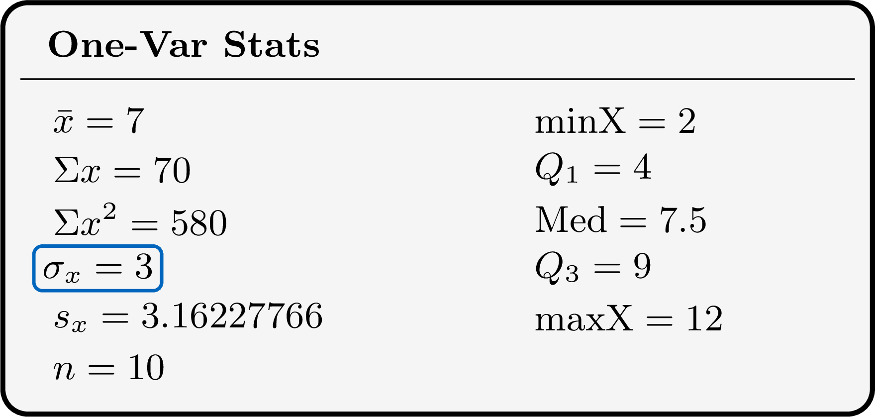
Calculators do not all compute the quartiles with the same convention — medians of the two halves, or values of the dataset — and some let the user choose. Entering \(1, 2, 3, 4\) shows which one a calculator uses: the medians of the halves give \(Q_1 = 1.5\), the values-of-the-dataset convention gives \(Q_1 = 1\).
Example
Ten pupils noted the time, in minutes, they spent on their homework one evening: $$35,\ 50,\ 20,\ 45,\ 60,\ 40,\ 30,\ 55,\ 45,\ 70.$$ Using a graphing calculator, find the mean, the standard deviation and the five-number summary of these times.
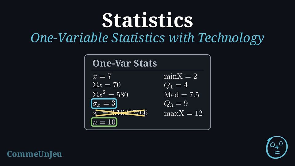
The ten times are typed in L1 and the one-variable statistics are run on L1. The screen shows: 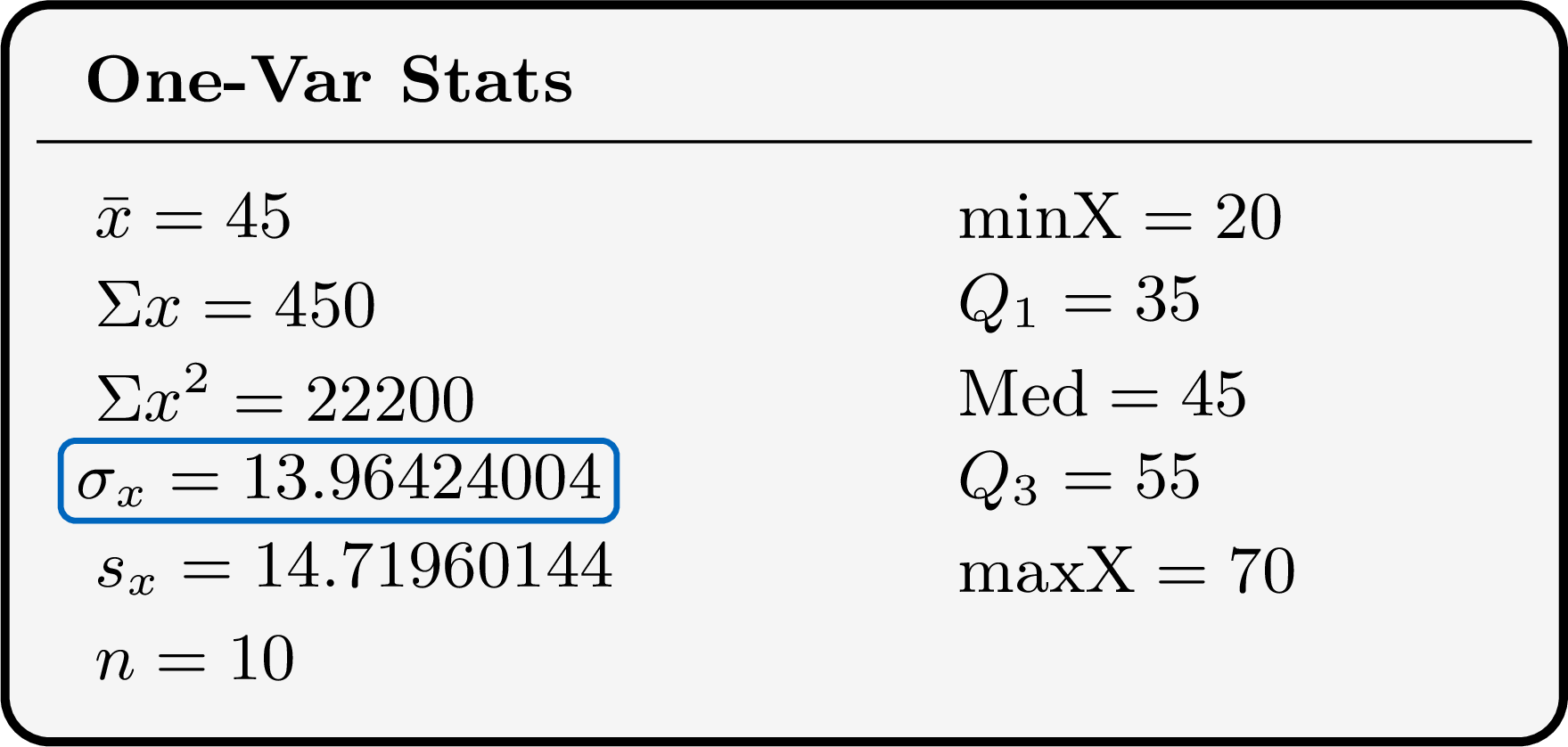
\(n = 10\): every value has been entered. The mean time is \(45\) minutes, the standard deviation is \(\sigma_x \approx 13.96\) minutes (not \(s_x\)), and the five-number summary is \(20, 35, 45, 55, 70\) minutes. With \(10\) values, both conventions for quartiles give \(Q_1 = 35\) and \(Q_3 = 55\) (the \(3^{\text{rd}}\) and \(8^{\text{th}}\) ordered values). A quick check of the mean: \(\frac{\Sigma x}{n} = \frac{450}{10} = 45\).
Example
A football team recorded the number of goals it scored in each of its \(22\) matches: | Goals | \(0\) | \(1\) | \(2\) | \(3\) | \(4\) | \(5\) |
| Matches | \(3\) | \(6\) | \(6\) | \(4\) | \(2\) | \(1\) |
The numbers of goals \(0, 1, 2, 3, 4, 5\) are typed in L1 and the numbers of matches \(3, 6, 6, 4, 2, 1\) in L2; the one-variable statistics are run with L1 as the data list and L2 as the frequency list. 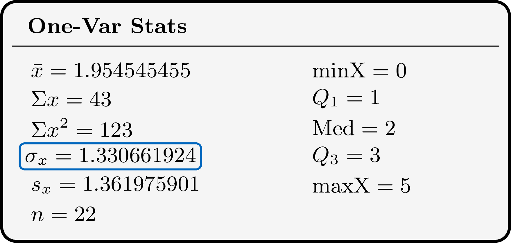
\(n = 22\) is the total number of matches: the frequency list has been taken into account. (Had it been forgotten, the calculator would have treated the six values \(0, \ldots, 5\) once each, and shown \(n = 6\).) The mean is about \(1.95\) goals per match, the standard deviation \(\sigma_x \approx 1.33\) goals; the quartiles are \(Q_1 = 1\), the median \(2\) and \(Q_3 = 3\) goals.
Example
The times, in minutes, that \(40\) pupils spent on a project were grouped in classes: | Time (min) | \([0, 10)\) | \([10, 20)\) | \([20, 30)\) | \([30, 40)\) | \([40, 50)\) |
| Pupils | \(4\) | \(9\) | \(12\) | \(10\) | \(5\) |
The exact times are unknown: each class is represented by its midpoint, the centre of the interval, as if all its values were equal to it. The midpoints \(5, 15, 25, 35, 45\) are typed in L1 and the frequencies \(4, 9, 12, 10, 5\) in L2. The screen gives \(n = 40\), \(\bar{x} = 25.75\) and \(\sigma_x = 11.70202974\). The mean time is estimated at about \(25.8\) minutes and the standard deviation at about \(11.7\) minutes. These are estimates, since every time of a class has been replaced by its midpoint. The quartiles shown on the same screen are midpoints of classes and are not used: the quartiles of grouped data are estimated on the cumulative frequency graph.
Skills to practice
- Using Technology for One-Variable Statistics
V.2
Linear Transformations of Data
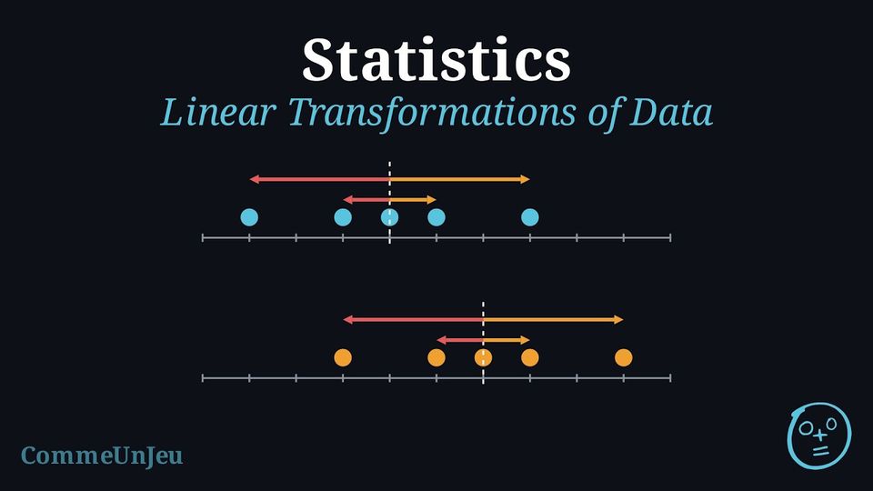
The marks, out of \(20\), of five pupils in a test are \(9, 11, 12, 13, 15\). Their mean is \(12\) and their standard deviation is \(2\).
- The teacher adds a bonus of \(2\) points to every mark. Compute the new mean and the new standard deviation.
- Instead, the marks are converted into marks out of \(40\) by doubling them. Compute the new mean and the new standard deviation.
- What do you notice?
- The new marks are \(11, 13, 14, 15, 17\); their mean is \(\frac{70}{5} = 14\). Their deviations from \(14\) are \(-3, -1, 0, 1, 3\) — exactly the deviations of the old marks from \(12\) — so $$\sigma = \sqrt{\frac{9 + 1 + 0 + 1 + 9}{5}} = \sqrt{4} = 2.$$
- The new marks are \(18, 22, 24, 26, 30\); their mean is \(\frac{120}{5} = 24\). Their deviations from \(24\) are \(-6, -2, 0, 2, 6\), twice the old ones, so $$\sigma = \sqrt{\frac{36 + 4 + 0 + 4 + 36}{5}} = \sqrt{16} = 4.$$
- Adding \(2\) to every mark adds \(2\) to the mean but does not change the standard deviation: the marks all move together, and their spread stays the same. Doubling every mark doubles both the mean and the standard deviation.
Proposition — Mean and Standard Deviation of a Linear Transformation
Let a dataset take the values \(x_1, \ldots, x_k\) with frequencies \(n_1, \ldots, n_k\) (total \(N\)), mean \(\bar{x}\), variance \(V_x\) and standard deviation \(\sigma_x\). Let \(a\) and \(b\) be two numbers. The dataset of the values \(y_i = a\,x_i + b\), each with the same frequency \(n_i\), has $$\bar{y} = a\,\bar{x} + b, \qquad V_y = a^2\,V_x, \qquad \sigma_y = |a|\,\sigma_x.$$ In particular: - adding the same number \(b\) to every value shifts the mean by \(b\) and leaves the standard deviation unchanged;
- multiplying every value by \(a\) multiplies the mean by \(a\) and the standard deviation by \(|a|\).
Mean. By the definition of the mean with frequencies, $$\begin{aligned}[t] \bar{y} &= \frac{1}{N}\sum_{i=1}^{k} n_i\,(a x_i + b) && \text{(definition of the mean)}\\
&= a \times \frac{1}{N}\sum_{i=1}^{k} n_i x_i + b \times \frac{1}{N}\sum_{i=1}^{k} n_i && \text{(expanding the sum)}\\
&= a\,\bar{x} + b. && \text{(}\textstyle\sum n_i x_i = N\bar{x}\text{ and }\sum n_i = N\text{)} \end{aligned}$$ This is the Proposition “Linearity of the Mean”, written with frequencies.
Deviations. Each deviation from the mean is multiplied by \(a\), and \(b\) disappears: $$y_i - \bar{y} = (a x_i + b) - (a\,\bar{x} + b) = a\,(x_i - \bar{x}).$$ Variance. $$\begin{aligned}[t] V_y &= \frac{1}{N}\sum_{i=1}^{k} n_i\,(y_i - \bar{y})^2 && \text{(definition of the variance)}\\ &= \frac{1}{N}\sum_{i=1}^{k} n_i\,a^2\,(x_i - \bar{x})^2 && \text{(}y_i - \bar{y} = a(x_i - \bar{x})\text{)}\\ &= a^2 \times \frac{1}{N}\sum_{i=1}^{k} n_i\,(x_i - \bar{x})^2 && \text{(factor } a^2\text{)}\\ &= a^2\,V_x. \end{aligned}$$ Standard deviation. $$\begin{aligned}[t] \sigma_y &= \sqrt{V_y} && \text{(definition of the standard deviation)}\\ &= \sqrt{a^2\,V_x}\\ &= \sqrt{a^2}\,\sqrt{V_x} && \text{(}a^2 \geq 0 \text{ and } V_x \geq 0\text{)}\\ &= |a|\,\sigma_x. && \text{(}\sqrt{a^2} = |a|\text{)} \end{aligned}$$ The shift \(b\) moves every value and the mean by the same amount, so it never reaches the deviations: that is why it does not change the spread.
Deviations. Each deviation from the mean is multiplied by \(a\), and \(b\) disappears: $$y_i - \bar{y} = (a x_i + b) - (a\,\bar{x} + b) = a\,(x_i - \bar{x}).$$ Variance. $$\begin{aligned}[t] V_y &= \frac{1}{N}\sum_{i=1}^{k} n_i\,(y_i - \bar{y})^2 && \text{(definition of the variance)}\\ &= \frac{1}{N}\sum_{i=1}^{k} n_i\,a^2\,(x_i - \bar{x})^2 && \text{(}y_i - \bar{y} = a(x_i - \bar{x})\text{)}\\ &= a^2 \times \frac{1}{N}\sum_{i=1}^{k} n_i\,(x_i - \bar{x})^2 && \text{(factor } a^2\text{)}\\ &= a^2\,V_x. \end{aligned}$$ Standard deviation. $$\begin{aligned}[t] \sigma_y &= \sqrt{V_y} && \text{(definition of the standard deviation)}\\ &= \sqrt{a^2\,V_x}\\ &= \sqrt{a^2}\,\sqrt{V_x} && \text{(}a^2 \geq 0 \text{ and } V_x \geq 0\text{)}\\ &= |a|\,\sigma_x. && \text{(}\sqrt{a^2} = |a|\text{)} \end{aligned}$$ The shift \(b\) moves every value and the mean by the same amount, so it never reaches the deviations: that is why it does not change the spread.
Example
Over the \(30\) days of a month, the daily maximum temperatures of a town have mean \(20\,^\circ\)C and standard deviation \(3\,^\circ\)C. A weather website converts every temperature into degrees Fahrenheit with \(F = 1.8\,C + 32\). Find the mean and the standard deviation of the temperatures in degrees Fahrenheit.
Every temperature is transformed by \(F = a\,C + b\) with \(a = 1.8\) and \(b = 32\). By the Proposition “Mean and Standard Deviation of a Linear Transformation”, $$\begin{aligned}[t] \bar{F} &= a\,\bar{C} + b = 1.8 \times 20 + 32 = 68 \,^\circ\text{F},\\
\sigma_F &= |a|\,\sigma_C = 1.8 \times 3 = 5.4 \,^\circ\text{F}. \end{aligned}$$ The \(+\,32\) moves every temperature, and the mean with it, but not the gaps between the temperatures: it plays no part in the standard deviation.
Example
In a game, a player starts each round with \(50\) points and loses \(2\) points per mistake, so the score of a round is \(y = 50 - 2x\), where \(x\) is the number of mistakes. Over a season, the numbers of mistakes per round have mean \(6\) and standard deviation \(2.5\). Find the mean and the standard deviation of the scores.
Here \(y = a\,x + b\) with \(a = -2\) and \(b = 50\). $$\begin{aligned}[t] \bar{y} &= a\,\bar{x} + b = -2 \times 6 + 50 = 38 \text{ points},\\
\sigma_y &= |a|\,\sigma_x = |-2| \times 2.5 = 5 \text{ points}. \end{aligned}$$ The standard deviation is \(5\), not \(-5\): a standard deviation is never negative. Multiplying by \(-2\) reverses the order of the scores (the more mistakes, the lower the score), but the gaps between scores are twice the gaps between numbers of mistakes.
Other Statistics Under a Linear Transformation
The same reasoning applies to the other statistics. When \(a > 0\), the order of the values is kept: the median and the quartiles are transformed like the values (\(\text{med}(y) = a\,\text{med}(x) + b\), and the same for \(Q_1\) and \(Q_3\)), while the range and the interquartile range, which are differences, are multiplied by \(a\) and do not depend on \(b\). When \(a < 0\), the order is reversed: the smallest values become the largest. The range is then multiplied by \(|a|\); the quartiles are best computed again on the new values, since the result depends on the convention used for the quartiles.
When \(\sigma_x > 0\), the standard score \(z = \dfrac{x - \bar{x}}{\sigma_x}\) is the linear transformation with \(a = \dfrac{1}{\sigma_x}\) and \(b = -\dfrac{\bar{x}}{\sigma_x}\): the standard scores of a dataset have mean \(0\) and standard deviation \(1\).
When \(\sigma_x > 0\), the standard score \(z = \dfrac{x - \bar{x}}{\sigma_x}\) is the linear transformation with \(a = \dfrac{1}{\sigma_x}\) and \(b = -\dfrac{\bar{x}}{\sigma_x}\): the standard scores of a dataset have mean \(0\) and standard deviation \(1\).
Skills to practice
- Updating the Mean and the Standard Deviation
- Justifying the Effect of a Linear Transformation
VI
Interpreting Data
VI.1
Drawing Conclusions and Evaluating Claims
Method — Interpreting Statistical Results
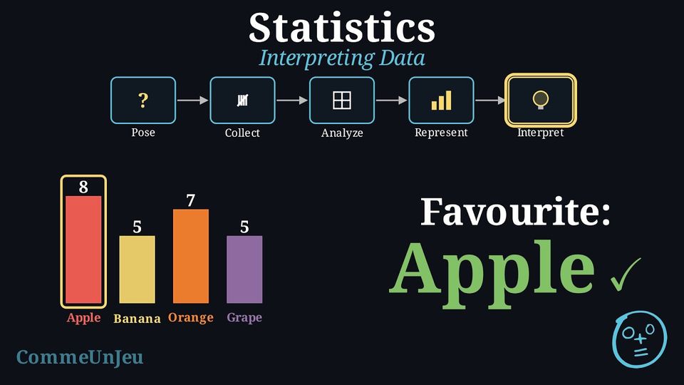
A rigorous interpretation of statistical results involves several steps: - Summarise Key Findings: State the principal results of the analysis, referencing descriptive statistics (e.g., mean, median, standard deviation) and key features of any graphical representations.
- Contextualise the Results: Relate the findings back to the original research question. What do these numbers mean in the context of the problem being studied?
- Make Inferences (If Applicable): If the data comes from a representative sample, make a careful inference about the wider population. It is crucial to acknowledge the uncertainty inherent in generalising from a sample to a population.
- Evaluate Limitations: Critically assess the limitations of the study. This includes considering potential sources of error (sampling error, selection bias, measurement error) and how they might affect the validity and generalisability of the conclusions.
Method — Critically Evaluating a Statistical Claim
When presented with a statistical claim, a critical evaluation should focus on two key areas: - Validity of the Data Collection: Was the sample representative of the target population, or could selection bias have influenced the results? Was the sample size adequate to support the conclusion? Were the questions neutral and unambiguous to avoid measurement error?
- Scope of the Conclusion: Does the conclusion overgeneralise the findings? A common error is to mistake a trend within a specific sample for a universal truth. A descriptive statistic (like a mean) summarises a group but does not apply to every individual within that group.
Example — Evaluating a Claim
Claim: “Girls are better at maths than boys.”Evidence Provided: A study of one class found that the girls' mean test score was 87\(\pourcent\), while the boys' mean was 75\(\pourcent\).
Critical Evaluation: The general claim is not justified by the evidence provided.
- Limitation of the Sample (Generalisation): The sample consists of only one class. It is not random and is too small to be considered representative of the entire population of “all girls” and “all boys”. The conclusion cannot be generalised beyond this specific group.
- Misinterpretation of Averages: The mean describes the central tendency of a group, not the performance of individuals. Even with a higher mean for the girls, some boys may well have scored higher than some girls — the means alone do not determine individual results. The claim “Girls are better” is an overgeneralisation that is easily read as true of every individual.
Skills to practice
- Judging Claims about Averages
VII
Going further
Skills to practice
- Solving Problems on Distributions without Technology
- Analysing Complete Data Sets with Technology
- Quiz
Jump to section