International Baccalaureate · DP 1: Analysis and Approaches HL
Probability
Master probability from basic outcomes to advanced concepts. Learn sample spaces, Venn diagrams, and addition laws. Deep dive into conditional probability, the law of total probability, and Bayes' Theorem using real-world scenarios like medical testing and forensic logic.
I
Sample Spaces
Definition — Outcome
An outcome is one possible result of a random experiment.Example
What are all the possible outcomes when you flip a coin?
The outcomes are Heads (H) =  and Tails (T) =
  .
.
Example
What are the outcomes when you roll a six-sided die?
The outcomes are\(1 = \) ,\(2 = \)
 ,\(3 = \)
 ,\(4 = \)
 ,\(5 = \)
 and \(6 = \)
 .
.
Definition — Sample Space
The sample space is the set of all possible outcomes of a random experiment.Example
What’s the sample space when you flip a coin?
The sample space is \(\{\text{Heads}, \text{Tails}\} = \{\),\(\}\), or just \(\{\text{H}, \text{T}\}\) for short.
Example
What’s the sample space when you roll a six-sided die?
The sample space is \(\{1, 2, 3, 4, 5, 6\} = \{\),,,,,\(\}\).
Skills to practice
- Finding the sample spaces
II
Events
Definition — Event
An event (often denoted by a capital letter like \(E\)) is a subset of the sample space.Example
For the experiment of rolling a die, list the outcomes in the event \(E\): “rolling an even number”.
Among the outcomes of the sample space \(\{1, 2, 3, 4, 5, 6\} = \{\),,,,,\(\}\), the event of rolling an even number is\(E = \{2, 4, 6\} = \{\),,\(\}\).
Skills to practice
- Finding Events for Die-Rolling Events
- Finding Events in a Casino Spinner
III
Complementary Events
In probability, it is often useful to consider the outcomes that do not belong to a specific event. This set of “other” outcomes is known as the complementary event. It represents everything in the sample space that is outside the original event. The complement of an event \(E\) is denoted by \(E'\).
Definition — Complementary Event
The complementary event of an event \(E\), denoted \(E'\), \(E^c\), or \(\overline{E}\), is the set of all outcomes in the sample space that are not in \(E\).Example
In the experiment of rolling a fair six-sided die, let \(E\) be the event “rolling an even number”. Find the complementary event, \(E'\).
The sample space is \(\{1, 2, 3, 4, 5, 6\} = \{\),,,,,\(\}\).
The event is \(E = \{2, 4, 6\} = \{\),,\(\}\).
The complementary event \(E'\) contains all outcomes in the sample space that are not in \(E\).
Therefore, \(E' = \{1, 3, 5\} = \{\),,\(\}\). This is the event “rolling an odd number”.
The event is \(E = \{2, 4, 6\} = \{\)
The complementary event \(E'\) contains all outcomes in the sample space that are not in \(E\).
Therefore, \(E' = \{1, 3, 5\} = \{\)
Skills to practice
- Finding the Complementary Events
IV
Multi-Step Random Experiments
A multi-step experiment is a random experiment made up of a sequence of two or more simple steps. For example, flipping two coins is a multi-step experiment composed of two actions: flipping the first coin and then flipping the second.
In many multi-step experiments, we can find the total number of possible outcomes by multiplying the number of outcomes at each step. To display all the combined outcomes, we can use tools like lists, tables, or tree diagrams.
In many multi-step experiments, we can find the total number of possible outcomes by multiplying the number of outcomes at each step. To display all the combined outcomes, we can use tools like lists, tables, or tree diagrams.
Method — Representing Sample Spaces for Multi-Step Experiments
When an experiment has more than one step, the sample space can be represented in several ways:- by listing all possible ordered outcomes;
- using a table (best for two-step experiments);
- using a tree diagram (useful for any number of steps).
Example
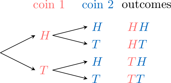
For the experiment of tossing two coins, represent the sample space by:- listing all possible outcomes;
- using a table;
- using a tree diagram.
- List:
Each outcome records the result of coin 1 first, then coin 2:$$\{\textcolor{colordef}{H}\textcolor{colorprop}{H}, \textcolor{colordef}{H}\textcolor{colorprop}{T}, \textcolor{colordef}{T}\textcolor{colorprop}{H}, \textcolor{colordef}{T}\textcolor{colorprop}{T}\}$$ - Table:
\(\begin{aligned} & \textcolor{colorprop}{\text{coin 2}} \\ \textcolor{colordef}{\text{coin 1}} \end{aligned} \) \(\textcolor{colorprop}{H}\) \(\textcolor{colorprop}{T}\) \(\textcolor{colordef}{H}\) \(\textcolor{colordef}{H}\textcolor{colorprop}{H}\) \(\textcolor{colordef}{H}\textcolor{colorprop}{T}\) \(\textcolor{colordef}{T}\) \(\textcolor{colordef}{T}\textcolor{colorprop}{H}\) \(\textcolor{colordef}{T}\textcolor{colorprop}{T}\) - Tree diagram:
Skills to practice
- Finding Outcome in a Table
- Counting the Number of Possible Outcomes in a Table
- Counting the Number of Possible Outcomes for an Event
- Counting the Number of Possible Outcomes in a Tree diagram
V
\(E\) or \(F\)
Definition — \(E\) or \(F\)
The union of two events \(E\) and \(F\), denoted \(E \cup F\), is the event that occurs if \(E\) occurs, or \(F\) occurs, or both occur. We read this as "E or F". It includes all outcomes that are in at least one of the events.Example
A standard six-sided die is rolled. Let event \(E\) be "rolling an even number" and event \(F\) be "rolling a number less than 4". Find the event \(E \cup F\).
The events are \(E = \{2, 4, 6\}\) and \(F = \{1, 2, 3\}\).
The union \(E \cup F\) contains all outcomes that appear in either set, without repetition:$$ E \cup F = \{1, 2, 3, 4, 6\}. $$
The union \(E \cup F\) contains all outcomes that appear in either set, without repetition:$$ E \cup F = \{1, 2, 3, 4, 6\}. $$
Skills to practice
- Finding the Union of Two Events in Dice Experiment
- Finding the Union of Two Events in Family Experiment
- Finding the Union of Two Events from a Table
VI
\(E\) and \(F\)
Definition — \(E\) and \(F\)
The intersection of two events \(E\) and \(F\), denoted \(E \cap F\), is the event that occurs if both \(E\) and \(F\) occur simultaneously. We read this as "E and F". It includes all outcomes that are common to both events.Example
A standard six-sided die is rolled. Let event \(E\) be "rolling an odd number" and event \(F\) be "rolling a number less than 4". Find the event \(E \cap F\).
The events are \(E = \{1, 3, 5\}\) and \(F = \{1, 2, 3\}\).
The intersection \(E \cap F\) contains only the outcomes that are in both sets:$$ E \cap F = \{1, 3\}. $$
The intersection \(E \cap F\) contains only the outcomes that are in both sets:$$ E \cap F = \{1, 3\}. $$
Skills to practice
- Finding the Intersection of Two Events in Dice Experiment
- Finding the Intersection of Two Events in Family Experiment
- Finding the Intersection of Two Events from a Table
VII
Mutually Exclusive
Definition — Mutually Exclusive
Two events \(E\) and \(F\) are mutually exclusive (or disjoint) if they have no outcomes in common. This means they cannot occur at the same time. Their intersection is the empty set (\(\emptyset\)):$$E \cap F = \emptyset.$$Example
When rolling a die, let \(E\) be the event "rolling an odd number" and \(F\) be the event "rolling an even number". Show that \(E\) and \(F\) are mutually exclusive.
The event sets are \(E = \{1, 3, 5\}\) and \(F = \{2, 4, 6\}\).
We find their intersection:$$ E \cap F = \emptyset. $$Since there are no outcomes common to both events, they are mutually exclusive.
We find their intersection:$$ E \cap F = \emptyset. $$Since there are no outcomes common to both events, they are mutually exclusive.
Skills to practice
- Determining Mutual Exclusivity
- Determining Mutual Exclusivity from Tables
VIII
Venn Diagram
Definition — Set Theory and Probability Vocabulary
| Notation | Set Vocabulary | Probability Vocabulary | Venn Diagram |
| \(U\) | Universal set | Sample space |  |
| \(x\) | Element of \(U\) | Outcome | 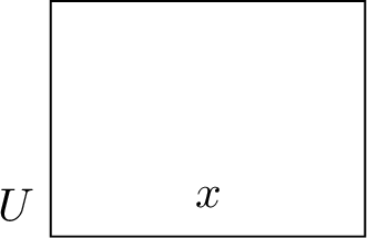 |
| \(\emptyset\) | Empty set | Impossible event | |
| \(E\) | Subset of \(U\) | Event | 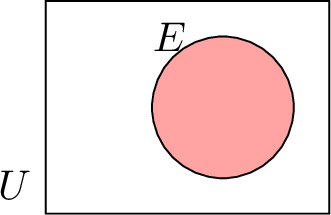 |
| \(x \in E\) | \(x\) is an element of \(E\) | \(x\) is an outcome of \(E\) | 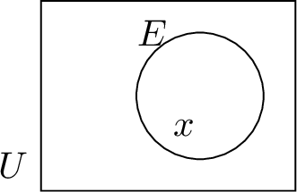 |
| \(E'\) | Complement of \(E\) in \(U\) | Complement of \(E\) in \(U\) | 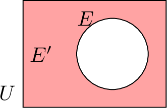 |
| \(E \text{ or } F\) | Union of \(E\) and \(F\): \(E \cup F\) | \(E\) or \(F\) | 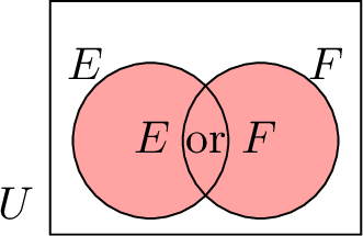 |
| \(E \text{ and } F\) | Intersection of \(E\) and \(F\): \(E \cap F\) | \(E\) and \(F\) | 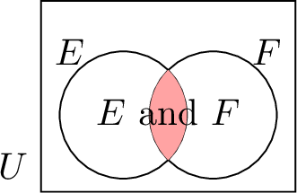 |
| \(E \cap F = \emptyset\) | \(E\) and \(F\) are disjoint | \(E\) and \(F\) are mutually exclusive | 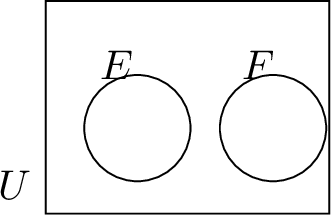 |
Skills to practice
- Finding the Union of Two Events in a Venn Diagram
- Finding the Intersection of Two Events in a Venn Diagram
IX
Axioms of Probability
When you flip a coin, there are two possible outcomes: heads or tails. The chance of getting heads is 1 out of 2. We can write this as a fraction: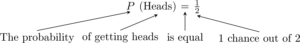
Definition — Probability
The probability of an event \(E\), written \(P(E)\), is a number that tells us how likely the event is to happen. It is always between \(0\) (impossible) and \(1\) (certain). In other words, for any event \(E\), we have \(0 \leq P(E) \leq 1\).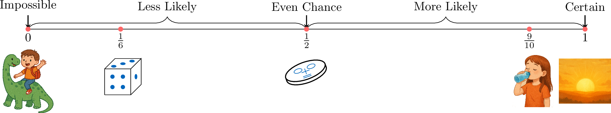
All of probability is built upon three fundamental rules called axioms. These are statements we accept as true and from which all other rules can be derived. The probability of an event \(E\), denoted \(P(E)\), is a number that quantifies its likelihood.
Definition — Probability Axioms
A function \(P\) is a probability measure if it satisfies the following three axioms for any events \(E\) and \(F\) in a sample space \(U\):- Axiom 1 (Non-negativity): The probability of any event is a non-negative number, between 0 and 1 inclusive. $$0 \leqslant P(E) \leqslant 1$$
- Axiom 2 (Total Probability): The probability of the entire sample space is 1. $$P(U) = 1$$
- Axiom 3 (Additivity for Mutually Exclusive Events): If two events \(E\) and \(F\) are mutually exclusive (\(E \cap F = \emptyset\)), then the probability of their union is the sum of their individual probabilities. $$P(E \cup F) = P(E) + P(F)$$
Visualizing the Axioms with Venn Diagrams
Venn diagrams can help us understand the probability axioms. In this context, the entire area of the universal set \(U\) is considered to have a total probability of 1. The probability of any event \(E\) is represented by the proportion of the total area that the event covers.
- Axiom 1: \(0 \leqslant P(E) \leqslant 1\)
The area representing event \(E\) cannot be smaller than nothing (0) and cannot be larger than the entire sample space (1).
- Axiom 2: \(P(U) = 1\)
It is certain that some outcome in the sample space occurs. Therefore, the probability of the entire sample space is 1 (or 100\(\pourcent\)).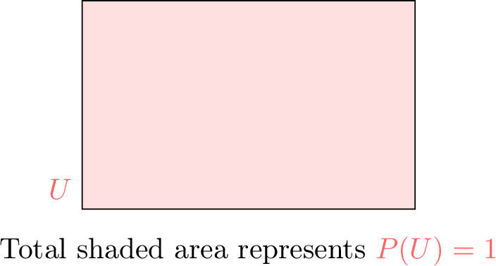
- Axiom 3: \(P(E \cup F) = P(E) + P(F)\) for Mutually Exclusive Events
If two events \(E\) and \(F\) are mutually exclusive, they do not overlap in the Venn diagram. The total area covered by their union (\(E \cup F\)) is simply the sum of their individual areas.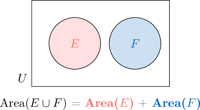
Skills to practice
- Describing Probabilities with Words
- Making Decisions Using Probabilities
- Finding Probability for Mutually Exclusive Events
X
Fundamental Probability Rules
If there is a \(40\pourcent\) chance of rain tomorrow, what is the chance that it will not rain?\(100\pourcent - 40\pourcent = 60\pourcent\) This calculation is an application of the complement rule. It is a shortcut to find the probability that an event does not happen.
Proposition — Complement Rule
For any event \(E\) and its complementary event \(E'\),$$\textcolor{colorprop}{P(E') = 1 - P(E)}$$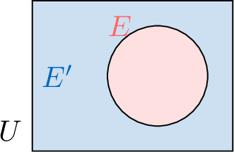
- Algebraic Proof
By definition, an event \(E\) and its complement \(E'\) are mutually exclusive (\(E \cap E' = \emptyset\)) and their union is the entire sample space (\(E \cup E' = U\)).
Using Axiom 3: \(P(E \cup E') = P(E) + P(E')\).
Using Axiom 2: \(P(U) = 1\).
Since \(E \cup E' = U\), we can equate their probabilities:$$ P(E) + P(E') = P(U) = 1. $$Rearranging the formula gives the complement rule:$$P(E') = 1 - P(E).$$ - Geometric Proof
The total area of the sample space, \(\textcolor{olive}{P(U)}\), ,is the sum of the area of the event, \textcolor{colordef}{\(P(E)\)}, and the area of its complement, \textcolor{colorprop}{\(P(E')\)}.
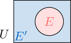
So,$$\textcolor{colordef}{P(E)} + \textcolor{colorprop}{P(E')} = \textcolor{olive}{P(U)}.$$Since \(\textcolor{olive}{P(U) = 1}\) (from Axiom 2), we have:$$\textcolor{colordef}{P(E)} + \textcolor{colorprop}{P(E')} = 1.$$
Example
Farid has a \(0.8\) (\(80\pourcent\)) chance of finishing his homework on time tonight (event \(E\)). What is the probability that he does not finish on time?
The complementary event \(E'\) is “Farid does not finish his homework on time”. Using the complement rule:$$\begin{aligned}P(E') &= 1 - P(E) \\
&= 1 - 0.8 \\
&= 0.2\end{aligned}$$There is a \(0.2\) (or \(20\pourcent\)) probability that he does not finish on time.
Proposition — Addition Law of Probability
For any two events \(E\) and \(F\),$$\textcolor{colorprop}{P(E \cup F) = P(E) + P(F) - P(E \cap F)}$$This formula holds whether or not \(E\) and \(F\) are mutually exclusive. If they are mutually exclusive, then \(P(E \cap F) = 0\) and the formula reduces to Axiom 3.
The Venn diagram below shows the sample space \(U\) with two intersecting events, \(E\) and \(F\).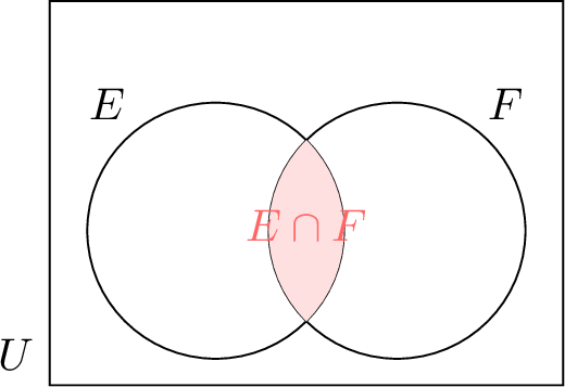
Therefore, the total probability of the union is$$P(E \cup F) = P(E) + P(F) - P(E \cap F).$$
Therefore, the total probability of the union is$$P(E \cup F) = P(E) + P(F) - P(E \cap F).$$
Example
A local high school is holding a talent show. The probability that a randomly selected student participates in singing is \(0.4\), the probability that a student participates in dancing is \(0.3\), and the probability that a student participates in both singing and dancing is \(0.1\). Find the probability that a randomly selected student participates in either singing or dancing.
Let \(S\) be the event "participates in singing" and \(D\) be the event "participates in dancing". We are given:
- \(P(S) = 0.4\)
- \(P(D) = 0.3\)
- \(P(S \cap D) = 0.1\)
Skills to practice
- Applying the Complement Rule
- Completing a Probability Tree Diagram
- Calculating Probabilities for Union of Events
- Calculating Probabilities for Union of Events in Real-World Problems
XI
Equally Likely
Have you ever flipped a fair coin or rolled a fair die? In these experiments, each outcome is just as likely as the others. We call these equally likely outcomes.
Definition — Equally Likely
When all outcomes are equally likely, the probability of an event \(E\) is:$$\textcolor{colordef}{\begin{aligned}P(E) &= \frac{\text{number of outcomes in the event}}{\text{number of outcomes in the sample space}}\\
&=\dfrac{\Card{E}}{\Card{U}}\\
\end{aligned}}$$Example
What’s the probability of rolling an even number with a fair six-sided die?- Sample space \(= \{1, 2, 3, 4, 5, 6\}\) (6 outcomes).
- \(E = \{2, 4, 6\}\) (3 outcomes).
- $$\begin{aligned}P(E) &= \frac{3}{6} \\ &= \frac{1}{2} \end{aligned}$$
Skills to practice
- Finding Probabilities in a Casino Spinner
- Finding Probabilities in a Dice Experiment
- Calculating the Probability In Multi-Step Random Experiments
XII
Probability of Independent Events
Independent events are events where knowing that one event has happened does not change the probability that the other event happens. For example, when rolling two fair dice at the same time, the result of the first die does not change the chances for the second die — they are independent events.
Definition — Independent Events
If two events, \(A\) and \(B\), are independent, the probability that both events happen (that is, \(P(A\cap B)\) or \(P(A \text{ and } B)\)) is the product of their individual probabilities. This is called the multiplication rule for independent events:$$P(A \text{ and } B) = P(A) \times P(B)$$Example
An experiment consists of the following two independent actions:- Tossing a fair coin.
- Rolling a fair six-sided die.
Let \(T\) be the event “getting tails” and \(N\) be the event “rolling a number greater than 4”.
- The events are independent, so we can use the multiplication rule.
- The probability of getting tails is \(P(T) = \dfrac{1}{2}\).
- The outcomes for a number greater than 4 are \(\{5, 6\}\). There are 2 favourable outcomes out of 6 total outcomes. So, \(P(N) = \dfrac{2}{6} = \dfrac{1}{3}\).
- Now, we multiply the probabilities to find the probability of both events happening:$$\begin{aligned}P(T \text{ and } N) &= P(T) \times P(N) \\ &= \dfrac{1}{2} \times \dfrac{1}{3} \\ &= \dfrac{1}{6}\end{aligned}$$
Method — Using a Probability Tree Diagram
- Draw branches for each step: Draw branches for the first event (coin toss) and then, from the end of each of those branches, draw the branches for the second event (die roll).
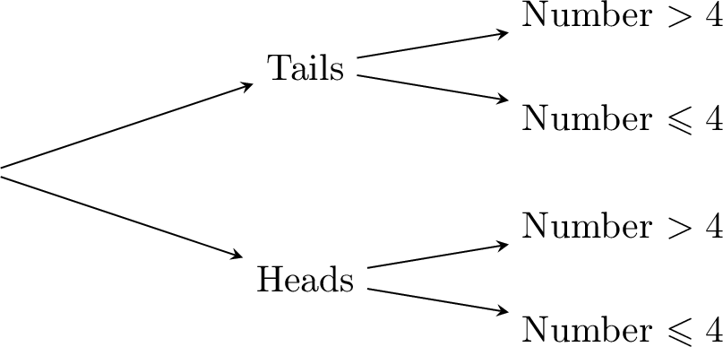
- Write probabilities on each branch: The probabilities on the branches from a single point must add up to 1. Because the events are independent, the probabilities on the die-roll branches are the same after “Tails” and after “Heads”.
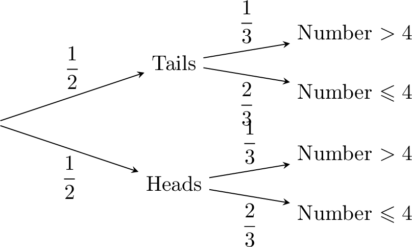
- Multiply along the path: To find the probability of a combined event, multiply the probabilities along the path from start to finish.
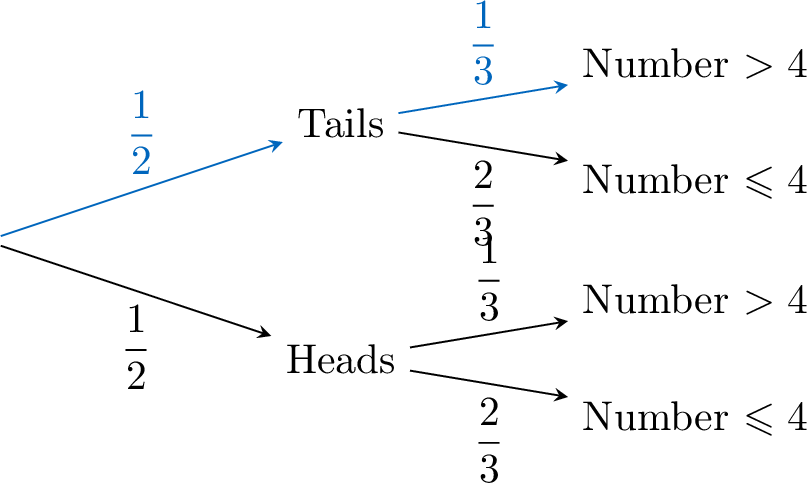 $$\textcolor{colorprop}{P(\text{"Tails" and "Number > 4"})=\frac{1}{2}\times \frac{1}{3}}$$
Skills to practice
- Draw a Probability Tree for Two Independent Events
- Calculating Probabilities from a Tree Diagram
- Calculating Probabilities from a Tree Diagram
- Calculating the Probability of Two Independent Events
XIII
Experimental Probability
Isaac wants to find the probability that a cone he drops will land on its base. The possible outcomes are “base down” or “on its side”.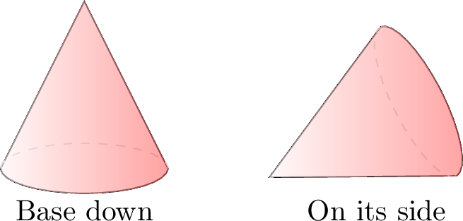
- Base down: 15 times.
- On its side: 35 times.
Definition — Experimental Probability (Relative Frequency)
The experimental probability of an event is an estimate found by repeating an experiment many times. It is calculated with the formula:$$ \text{Experimental Probability} = \frac{\text{Number of times an event occurs}}{\text{Total number of trials}} $$The more trials we do, the better our estimate of the true probability will be.Skills to practice
- Calculating Experimental Probabilities in Percentage Form
- Conducting Experiments to Estimate Probabilities
XIV
Definition
Let’s explore conditional probability with a two-way table showing 100 students’ preferences for math, split by gender:
| Loves Math | Does Not Love Math | Total | |
| Girls | 35 | 16 | 51 |
| Boys | 30 | 19 | 49 |
| Total | 65 | 35 | 100 |
- Probability the student is a girl:$$\begin{aligned}P(\text{Girl}) &= \frac{\text{Number of girls}}{\text{Number of students}} \\ &= \frac{51}{100}.\end{aligned}$$
- Probability the student loves math and is a girl:$$\begin{aligned}P(\text{Loves Math and Girl}) &= \frac{\text{Number of girls who love math}}{\text{Number of students}} \\ &= \frac{35}{100}.\end{aligned}$$
- Probability the student loves math, given they are a girl:
Since we’re told the student is a girl, we focus only on the 51 girls:$$\begin{aligned}\PCond{\text{Loves Math}}{\text{Girl}} &= \frac{\text{Number of girls who love math}}{\text{Number of girls}} \\ &= \frac{35}{51}.\end{aligned}$$ - Connecting to the formula:
Notice that:$$\begin{aligned}\PCond{\text{Loves Math}}{\text{Girl}} &=\frac{35}{51}\\ &= \frac{35/100}{51/100}\\ &= \dfrac{P(\text{Loves Math and Girl})}{P(\text{Girl})}.\end{aligned}$$This pattern gives us the general rule for conditional probability.
Definition — Conditional Probability
The conditional probability of event \(F\) given event \(E\) is the probability of \(F\) occurring, knowing that \(E\) has already happened. It’s denoted \(\PCond{F}{E}\) and calculated as:$$\textcolor{colordef}{\PCond{F}{E} = \frac{P(E \cap F)}{P(E)}}, \quad \text{where } P(E) > 0.$$Example
A fair six-sided die has odd faces (1, 3, 5) painted green and even faces (2, 4, 6) painted blue. You roll it and see the top face is blue. What’s the probability it’s a 6?- Sample space: \(\{1, 2, 3, 4, 5, 6\}\), 6 equally likely outcomes.
- Event \(E\) (face is blue): \(\{2, 4, 6\}\), so \(P(E) = \frac{3}{6}\).
- Event \(F\) (roll a 6): \(\{6\}\).
- Intersection \(E \cap F\): \(\{6\}\), so \(P(E \cap F) = \frac{1}{6}\).
- Conditional probability:$$\begin{aligned}\PCond{F}{E} &= \frac{P(E \cap F)}{P(E)}\\ &= \frac{\frac{1}{6}}{\frac{3}{6}}\\ &= \frac{1}{6} \times \frac{6}{3}\\ &= \frac{1}{3}.\end{aligned}$$
- The probability of rolling a 6, given the face is blue, is \(\frac{1}{3}\).
Skills to practice
- Exploring Probabilities with Two-Way Tables
- Calculating Conditional Probabilities
- Calculating Conditional Probabilities in Real-World Problems
XV
Conditional Probability Tree Diagrams
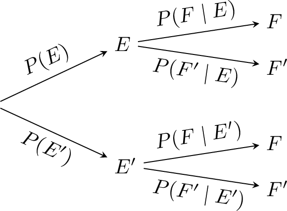
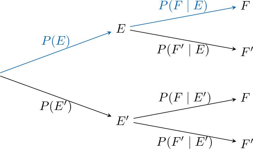
Definition — Conditional Probability Tree Diagram
A conditional probability tree visually organizes probabilities for a sequence of events:- Each branch from a node shows either an unconditional probability (e.g. \(P(E)\)) or a conditional probability (e.g. \(\PCond{F}{E}\)).
- Events are labeled at the end of each branch.
- The probability of an outcome at the end of a path is the product of the probabilities along that path.
Example
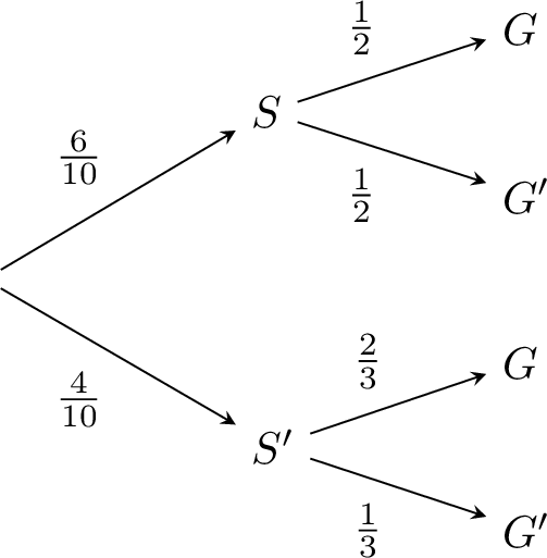
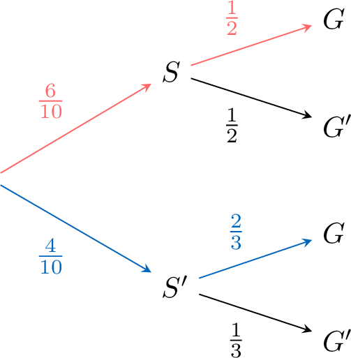
The probability Sam coaches a game is \(\frac{6}{10}\), and the probability Alex coaches is \(\frac{4}{10}\). If Sam coaches, the probability that a randomly selected player is a goalkeeper is \(\frac{1}{2}\); if Alex coaches, it is \(\frac{2}{3}\).Draw the tree diagram.
- Define the events:
- \(S\): Sam coaches.
- \(G\): Player is goalkeeper.
- Define the probabilities:
- \(P(S) = \frac{6}{10}\) and \(P(S') =1 - P(S)= \frac{4}{10}\).
- \(\PCond{G}{S} = \frac{1}{2}\) and \(\PCond{G'}{S} = 1 - \PCond{G}{S} = \frac{1}{2}\).
- \(\PCond{G}{S'} = \frac{2}{3}\) and \(\PCond{G'}{S'} = 1-\PCond{G}{S'}= \frac{1}{3}\).
- Tree diagram:
Skills to practice
- Identifying Conditional Probability Tree Diagrams
- Drawing Conditional Probability Tree Diagrams
XVI
Joint Probability: \(P(E \cap F)\)
Sometimes we know \(P(E)\) and \(\PCond{F}{E}\) and need the chance both \(E\) and \(F\) happen together—like finding the probability that a student is a girl who loves math. This probability is called the joint probability \(P(E \cap F)\).
Proposition — Joint Probability Formula
$$P(E \cap F) = P(E) \times \PCond{F}{E}, \quad P(E \cap F) = P(F) \times \PCond{E}{F}.$$Method — Finding \(P(E \cap F)\) in a Tree
- Identify the path where \(E\) and \(F\) both occur.
- Multiply the probabilities along that path.
Example
For this probability tree,- Path: \(S\) to \(G\) (highlighted):
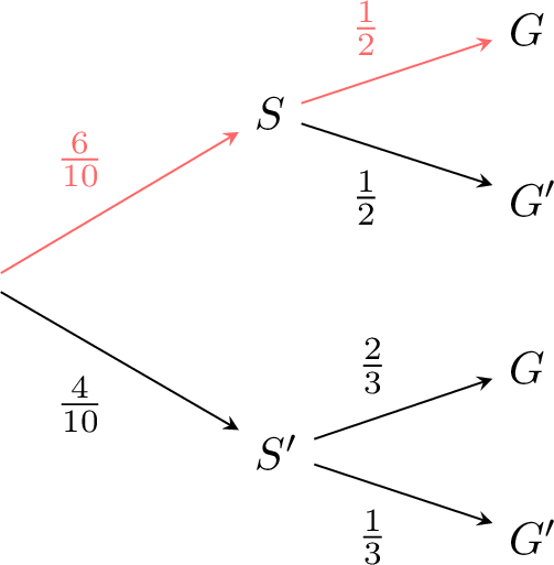
- Calculate:$$\begin{aligned}P(S \cap G) &= P(S) \times \PCond{G}{S}\\ &= \frac{6}{10} \times \frac{1}{2}\\ &= \frac{3}{10}.\end{aligned}$$
Skills to practice
- Calculating Joint Probabilities with Trees
XVII
Law of Total Probability
Theorem — Law of Total Probability
For events \(E\) and \(F\):$$P(F) = P(E) \PCond{F}{E} + P(E') \PCond{F}{E'}.$$This applies when \(E\) and its complement \(E'\) form a partition of the sample space. More generally, if \((E_1,\dots,E_n)\) is a partition of the sample space, then$$P(F) = \sum_{i=1}^n P(E_i)\PCond{F}{E_i}.$$Method — Finding \(P(F)\) in a Tree
- Identify all paths to \(F\).
- Multiply probabilities along each path and sum them.
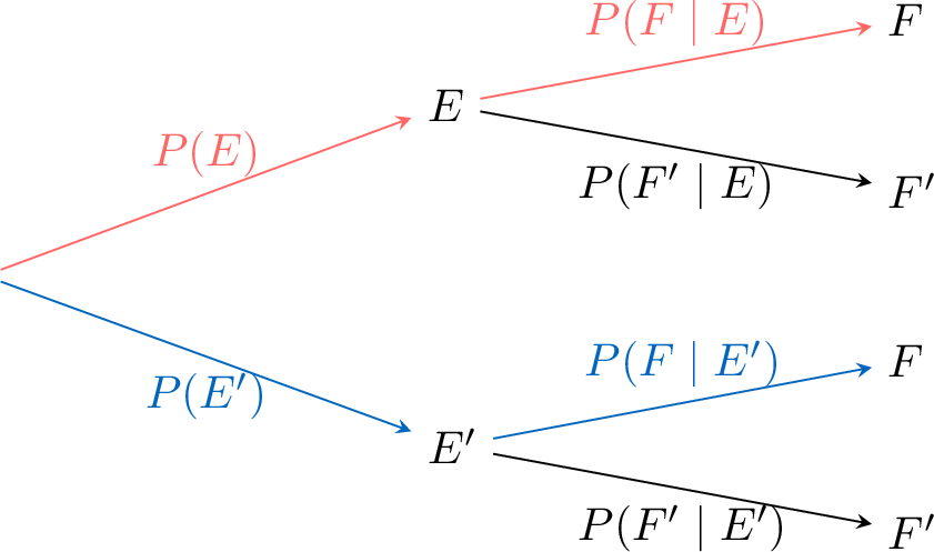
Example
For this probability tree,- Paths to \(G\):
- Calculate:$$\begin{aligned}P(G) &= \textcolor{colordef}{\frac{6}{10} \times \frac{1}{2}} + \textcolor{colorprop}{\frac{4}{10} \times \frac{2}{3}} \\ &= \textcolor{colordef}{\frac{3}{10}} + \textcolor{colorprop}{\frac{8}{30}} \\ &= \textcolor{colordef}{\frac{9}{30}} + \textcolor{colorprop}{\frac{8}{30}} \\ &= \frac{17}{30}.\end{aligned}$$
Skills to practice
- Calculating Probabilities with Trees
- Calculating Probabilities in Real-World Problems
XVIII
Bayes’ Theorem
What if you test positive for a rare disease—does that mean you have it? Bayes’ Theorem helps us flip conditional probabilities to answer questions like this, updating our beliefs with new evidence. It’s a cornerstone in fields like medicine and data science.
Theorem — Bayes’ Theorem
$$\PCond{E}{F} = \frac{P(E) \PCond{F}{E}}{P(F)}, \quad \text{where } P(F) > 0.$$Using the law of total probability for \(P(F)\), when \(\{E,E'\}\) is a partition of the sample space, this can also be written as$$\PCond{E}{F} = \frac{P(E)\PCond{F}{E}}{P(E)\PCond{F}{E} + P(E')\PCond{F}{E'}}.$$Example
Consider a rare disease that affects approximately 1 in every 1,000 people. A medical test developed for detecting this disease has the following characteristics:- Sensitivity: If a person has the disease, the test correctly returns a positive result 99\(\pourcent\) of the time.
- Specificity: If a person does not have the disease, the test correctly returns a negative result 95\(\pourcent\) of the time.
Define the following events clearly: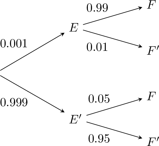
- Event \(E\): The person has the disease.
- Event \(F\): The test result is positive.
- \(P(E) = \frac{1}{1000} = 0.001\), thus \(P(E') = 1 - 0.001 = 0.999\).
- \(\PCond{F}{E} = 0.99\), hence \(\PCond{F'}{E} = 1 - 0.99 = 0.01\).
- \(\PCond{F'}{E'} = 0.95\), hence \(\PCond{F}{E'} = 1 - 0.95 = 0.05\).
Skills to practice
- Unveiling the Hidden Cause: Bayes' Theorem in Rare Event Detection
XIX
Review \& Beyond
Skills to practice
- Quiz
Jump to section