French National Education · Grade 12 Expert
Markov Chains
Master Markov Chains through stochastic modeling. Covers the Markov property, transition diagrams, and matrix formalism (πn = π0 * M^n). Includes exercises on system evolution and steady states using real scenarios like market shares and car rentals.
I
Markov Property
To model a system over time, we consider a sequence of random variables \((X_0, X_1, X_2, \dots)\). Each variable \(X_n\) represents the state of the system at step \(n\). The defining feature of a Markov chain is that the probability of moving to a future state depends only on the current state, and not on the past history of the system.
Definition — State Space and Markov Property
Let \(E\) be a finite set \(\{e_1, e_2, \dots, e_k\}\) called the state space.A sequence of random variables \((X_n)_{n \in \mathbb{N}}\) taking values in \(E\) is a Markov chain if, for all \(n \in \mathbb{N}\), for all indices \(i,j \in \{1,\dots,k\}\), and for all indices \(i_0,\dots,i_{n-1} \in \{1,\dots,k\}\) such that the conditioning event has positive probability,$$P\!\Bigl(X_{n+1}=e_j \,\Big|\, X_n=e_i,\; X_{n-1}=e_{i_{n-1}},\dots,\; X_0=e_{i_0}\Bigr)=P\!\Bigl(X_{n+1}=e_j \,\Big|\, X_n=e_i\Bigr).$$In this chapter, we consider time-homogeneous Markov chains, i.e.\ the conditional probability$$p_{ij}=P\!\bigl(X_{n+1}=e_j \mid X_n=e_i\bigr)$$does not depend on \(n\). The number \(p_{ij} \in [0, 1]\) is the transition probability from state \(e_i\) to state \(e_j\).
Method — From Natural Language to a Markov Chain Model
When a situation is described in everyday language, we build a Markov chain model by following these steps:- Identify the time steps. Decide what one step represents (one day, one week, one transaction, etc.).
- Choose the states. List the possible situations the system can be in at each step (finite set \(E=\{e_1,\dots,e_k\}\)).
- Index the states. Fix an order on \(E\) and associate each state with an index: $$ e_1 \leftrightarrow 1,\quad e_2 \leftrightarrow 2,\quad \dots,\quad e_k \leftrightarrow k. $$ This indexing will be used to build vectors and matrices.
- Define the random variables. Introduce \((X_n)_{n\in\mathbb{N}}\) where \(X_n\) is the state at time \(n\), taking values in \(E\).
- Translate the “memoryless” assumption. Express that the future depends only on the present: $$ P(X_{n+1}=e_j \mid X_n=e_i,\dots,X_0=e_{i_0})=P(X_{n+1}=e_j \mid X_n=e_i). $$
- Extract transition probabilities. For each pair \((i,j)\), define $$ p_{ij}=P(X_{n+1}=e_j\mid X_n=e_i). $$
Example — Weather Model - States (with indexing)
- Natural Language.
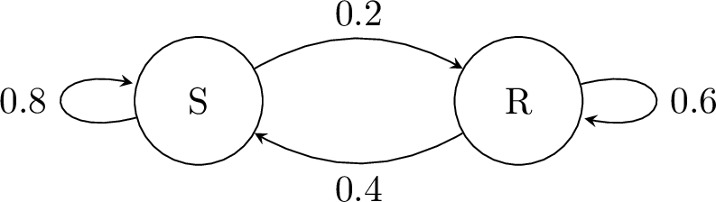
Consider the weather in a city. Each day, the weather is either sunny or rainy. Suppose that:- if it is sunny today, then the probability that it rains tomorrow is \(0.2\);
- if it is rainy today, then the probability that it is sunny tomorrow is \(0.4\).
- Mathematical Formalism.
We take one time step to be one day. We choose two states:$$e_1=S \quad (\text{Sunny}), \qquad e_2=R \quad (\text{Rainy}),$$so the state space is \(E=\{e_1,e_2\}=\{S,R\}\), with indexing$$S \leftrightarrow 1,\qquad R \leftrightarrow 2.$$We define \((X_n)_{n\in\mathbb{N}}\) by letting \(X_n\) be the weather on day \(n\), with values in \(E\). The phrase “independent of the weather on previous days” is modeled by the Markov property. The transition probabilities are then:$$p_{12}=P(X_{n+1}=e_2\mid X_n=e_1)=P(X_{n+1}=R\mid X_n=S)=0.2,$$$$p_{21}=P(X_{n+1}=e_1\mid X_n=e_2)=P(X_{n+1}=S\mid X_n=R)=0.4.$$Since the probabilities leaving a state sum to \(1\), we also obtain:$$p_{11}=1-p_{12}=0.8, \qquad p_{22}=1-p_{21}=0.6.$$Thus, all transition probabilities are$$p_{11}=0.8,\quad p_{12}=0.2,\quad p_{21}=0.4,\quad p_{22}=0.6.$$
Definition — Probabilistic Graph
A Markov chain can be visualized using a probabilistic graph:- Each node represents a state in \(E\).
- Each directed edge (arrow) from \(i\) to \(j\) represents the transition \(i \to j\).
- The weight on the edge is the probability \(p_{ij}\).
- Rule: The sum of probabilities on arrows leaving any node must be 1.
Example — Weather Graph
Skills to practice
- Analyzing the Markov Property
- Modeling a Simple Transition
- Analyzing the Probabilistic Graphs
- Reading Probabilistic Graphs
- Constructing Transition Diagrams
II
Matrix Formalism
To perform calculations, we associate each state with an index (typically \(1,2,\dots,k\)). This allows us to organize transition probabilities into vectors and matrices, and to use matrix multiplication to study the evolution of the system.
Definition — Probability Vector
The probability distribution at step \(n\) is represented by a row vector \(\pi_n\):$$\pi_n = \begin{pmatrix} P(X_n = e_1) & P(X_n = e_2) & \dots & P(X_n = e_k) \end{pmatrix}.$$Each component is in \([0,1]\), and the sum of the components is always 1. The vector \(\pi_0\) is called the initial distribution.Definition — Transition Matrix
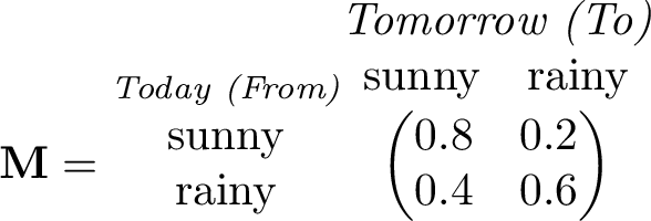
The transition matrix \(\mathbf{M}\) is a square matrix whose entry \(m_{ij}\) in the \(i\)-th row and \(j\)-th column is:$$m_{ij} = P(X_{n+1} = e_j \mid X_n = e_i)=p_{ij}.$$Stochastic Matrix: In this curriculum, the sum of each row of \(\mathbf{M}\) is 1.
In a transition matrix \(\mathbf{M} = (m_{ij})\):
- The rows represent the current state (From).
- The columns represent the next state (To).
- The entry \(m_{ij}\) represents the probability of moving to state \(j\) starting from state \(i\).
- The sum of each row must be 1.
Example — Weather Transition Matrix
Let State 1 = Sunny (\(S\)) and State 2 = Rainy (\(R\)). If today is definitely Sunny, the initial vector is \(\pi_0 = \begin{pmatrix} 1 & 0 \end{pmatrix}\).The matrix is:
Skills to practice
- Analyzing the Matrix Representation
- Defining and Validating Probability Vectors
- Constructing and Reading Transition Matrices
III
Evolution of the System
Once the transition matrix is defined, we can compute the distribution of the system at any time \(n\) using matrix multiplication.
Proposition — Evolution Rule
For a Markov chain with transition matrix \(\mathbf{M}\) and probability vector \(\pi_n\):$$\pi_{n+1} = \pi_n \mathbf{M}\quad \text{and, by induction,} \quad\pi_n = \pi_0 \mathbf{M}^n.$$
We prove the relationship in two steps: first the recursive relation, then the general form by induction.
- Proof of \(\pi_{n+1} = \pi_n \mathbf{M}\): Let \(E = \{1, 2, \dots, k\}\) be the state space. By the Law of Total Probability, for any state \(j \in E\): $$ P(X_{n+1} = j) = \sum_{i=1}^{k} P(X_n = i \cap X_{n+1} = j) $$ Using the definition of conditional probability: $$ P(X_{n+1} = j) = \sum_{i=1}^{k} P(X_n = i) \times P(X_{n+1} = j \mid X_n = i) $$ In terms of our notations:
- \(P(X_n = i)\) is the \(i\)-th component of the vector \(\pi_n\).
- \(P(X_{n+1} = j \mid X_n = i)\) is the coefficient \(m_{ij}\) of the transition matrix \(\mathbf{M}\).
- Proof of \(\pi_n = \pi_0 \mathbf{M}^n\) by induction:
- Initialization: For \(n=0\), \(\pi_0 \mathbf{M}^0= \pi_0 \mathbf{I} =\pi_0 \). The property is true.
- Heredity: Suppose that for a given \(n \in \mathbb{N}\), \(\pi_n = \pi_0 \mathbf{M}^n\). $$ \begin{aligned} \pi_{n+1} &= \pi_n \times \mathbf{M} \\ &= (\pi_0 \times \mathbf{M}^n) \times \mathbf{M} \quad (\text{by the induction hypothesis}) \\ &= \pi_0 \times \mathbf{M}^{n+1}. \end{aligned} $$
- Conclusion: By induction, for all \(n \in \mathbb{N}\), \(\pi_n = \pi_0 \mathbf{M}^n\).
Proposition — Coefficient \((i,j)\) of \(\mathbf{M}^n\)
Let \(\mathbf{M}\) be the transition matrix of a Markov chain \((X_n)\).The coefficient at the \(i\)-th row and \(j\)-th column of the matrix \(\mathbf{M}^n\), denoted \((\mathbf{M}^n)_{ij}\), is the probability of being in state \(j\) after \(n\) steps, given that the system started in state \(i\):$$ (\mathbf{M}^n)_{ij} = P(X_n = j \mid X_0 = i) $$
Example — Weather Prediction
Today it is sunny. Find the probability that it will be sunny the day after tomorrow.- Method with Step-by-Step Evolution: Using our weather matrix \(\mathbf{M} = \begin{pmatrix} 0.8 & 0.2 \\ 0.4 & 0.6 \end{pmatrix}\) and \(\pi_0 = \begin{pmatrix} 1 & 0 \end{pmatrix}\):$$\pi_1 = \pi_0 \mathbf{M}= \begin{pmatrix} 1 & 0 \end{pmatrix}\begin{pmatrix} 0.8 & 0.2 \\ 0.4 & 0.6 \end{pmatrix}= \begin{pmatrix} 0.8 & 0.2 \end{pmatrix}.$$The distribution in 2 days (\(n=2\)):$$\pi_2 = \pi_1 \mathbf{M}= \begin{pmatrix} 0.8 & 0.2 \end{pmatrix}\begin{pmatrix} 0.8 & 0.2 \\ 0.4 & 0.6 \end{pmatrix}= \begin{pmatrix} 0.72 & 0.28 \end{pmatrix}.$$Thus, there is a \(72\pourcent\) chance that it will be sunny the day after tomorrow.
- Method with Matrix Powers:Calculate \(\mathbf{M}^2\):$$\mathbf{M}^2 = \begin{pmatrix} 0.8 & 0.2 \\ 0.4 & 0.6 \end{pmatrix} \begin{pmatrix} 0.8 & 0.2 \\ 0.4 & 0.6 \end{pmatrix} = \begin{pmatrix} \mathbf{0.72} & 0.28 \\ 0.56 & 0.44 \end{pmatrix}$$The coefficient \((\mathbf{M}^2)_{11} = 0.72\) gives \(P(X_2=S \mid X_0=S) = \mathbf{0.72}\).
Skills to practice
- Analyzing the Evolution of a Markov Chain
- Calculating and Predicting States after One Step
- Calculating and Predicting States after Two Steps
- Calculating Successive Distributions
IV
Steady State and Convergence
Over a long period, many Markov chains approach an equilibrium in which the distribution no longer changes from one step to the next. This limit distribution is called the steady state (or stationary distribution).
Definition — Steady State
A probability vector \(\pi\) is a steady state (or stationary distribution) if:$$\pi \mathbf{M} = \pi.$$Method — Calculating the Steady State
To find \(\pi = \begin{pmatrix} x & y \end{pmatrix}\) for a 2-state matrix:- Solve the matrix equation \(\begin{pmatrix} x & y \end{pmatrix} \mathbf{M} = \begin{pmatrix} x & y \end{pmatrix}\).
- This leads to a system of linear equations; one equation is redundant.
- Add the normalization condition: \(x + y = 1\).
Example — Weather Steady State
For \(M = \begin{pmatrix} 0.8 & 0.2 \\ 0.4 & 0.6 \end{pmatrix}\), solving \(\begin{cases}\pi \mathbf{M} = \pi\\x + y = 1\end{cases}\quad\text{with}\quad\pi=\begin{pmatrix} x & y \end{pmatrix}\) gives$$\begin{cases}\begin{pmatrix} x & y \end{pmatrix} \begin{pmatrix} 0.8 & 0.2 \\
0.4 & 0.6 \end{pmatrix} = \begin{pmatrix} x & y \end{pmatrix}\\
x + y = 1\end{cases}\Leftrightarrow\begin{cases}0.8x + 0.4y = x \\
0.2x + 0.6y = y \\
x + y = 1\end{cases}\Leftrightarrow\begin{cases}-0.2x+0.4y=0 \\
x + y = 1\end{cases}\Leftrightarrow\begin{cases}x = 2y \\
3y = 1\end{cases}$$The steady state is$$\pi=\begin{pmatrix} \dfrac{2}{3} & \dfrac{1}{3} \end{pmatrix}.$$Interpretation: in the long run, the probability of being in state \(S\) (Sunny) is \(\dfrac{2}{3}\).Skills to practice
- Analyzing Steady States and Convergence
- Calculating Steady States
- From Probabilistic Graphs to Steady States
V
Review \& Beyond
Skills to practice
- Quiz
Jump to section