Differential Equations
Many of the most important laws of nature, from the motion of planets to the growth of populations, are described not by simple formulas but by equations that relate a function to its rates of change. These are known as differential equations. They form the language of modern science and engineering.
In this chapter, we will learn what differential equations are and explore several fundamental techniques for finding their solutions. We will begin with analytical methods for exact solutions, such as separation of variables and the integrating factor method. We will then investigate numerical methods, like Euler's method, which allow us to approximate solutions when exact ones are out of reach. Finally, we will see how these equations are applied to model real-world phenomena like logistic growth and Newton's law of cooling.
In this chapter, we will learn what differential equations are and explore several fundamental techniques for finding their solutions. We will begin with analytical methods for exact solutions, such as separation of variables and the integrating factor method. We will then investigate numerical methods, like Euler's method, which allow us to approximate solutions when exact ones are out of reach. Finally, we will see how these equations are applied to model real-world phenomena like logistic growth and Newton's law of cooling.
Fundamentals of Differential Equations
Definition Differential Equation
A differential equation is an equation that contains an unknown function and one or more of its derivatives.
- The order of a differential equation is the order of the highest derivative it contains.
- A general solution is a family of functions that satisfies the equation, typically involving one or more arbitrary constants.
- An initial condition is a specified value of the function or its derivatives at a particular point.
- A particular solution is a specific solution. It can be obtained by using an initial condition to determine the values of the arbitrary constants in the general solution.
Example
An apple is dropped from rest at a height of 10 meters. Its vertical position, \(y(t)\), is governed by the second-order differential equation:$$\frac{d^2 y}{dt^2}=-g$$where \(g\) is the constant of gravitational acceleration.
- State the initial conditions for position \(y(0)\) and velocity \(y'(0)\).
- Verify that the general solution to this equation is \(y(t) = -\frac{1}{2}gt^2 + At + B\).
- Use the initial conditions to find the particular solution for the apple's motion.
- Initial Conditions:
- The initial height is 10 meters, so \(y(0)=10\).
- The apple is dropped ``from rest,'' so its initial velocity is zero. Thus, \(y'(0)=0\).
- Verifying the General Solution: We need to show that the second derivative of \(y(t) = -\frac{1}{2}gt^2 + At + B\) is equal to \(-g\).
- First derivative (velocity): \(y'(t) = \dfrac{d}{dt}\left(-\frac{1}{2}gt^2 + At + B\right) = -gt + A\).
- Second derivative (acceleration): \(y''(t) = \dfrac{d}{dt}(-gt + A) = -g\).
- Finding the Particular Solution: We apply the initial conditions to the general solution and its first derivative.
- Using \(y(0)=10\): $$ y(0) = -\frac{1}{2}g(0)^2 + A(0) + B \implies 10 = B $$
- Using \(y'(0)=0\): $$ y'(0) = -g(0) + A \implies 0 = A $$
Slope Fields
While algebraic techniques give us formulas for solutions, a geometric approach can give us a powerful intuition for how solutions behave. A differential equation of the form \(\dfrac{dy}{dx} = f(x, y)\) is a machine that gives us the slope of a solution curve at any point \((x,y)\) in the plane.
A slope field (or direction field) is a graphical representation of this information. At each point on a grid, we draw a small line segment with the slope given by the differential equation. The resulting field of slopes acts like a set of ``currents'' in a river. Any particular solution to the differential equation is a curve that ``flows'' along these currents, always tangent to the slope markers it passes through.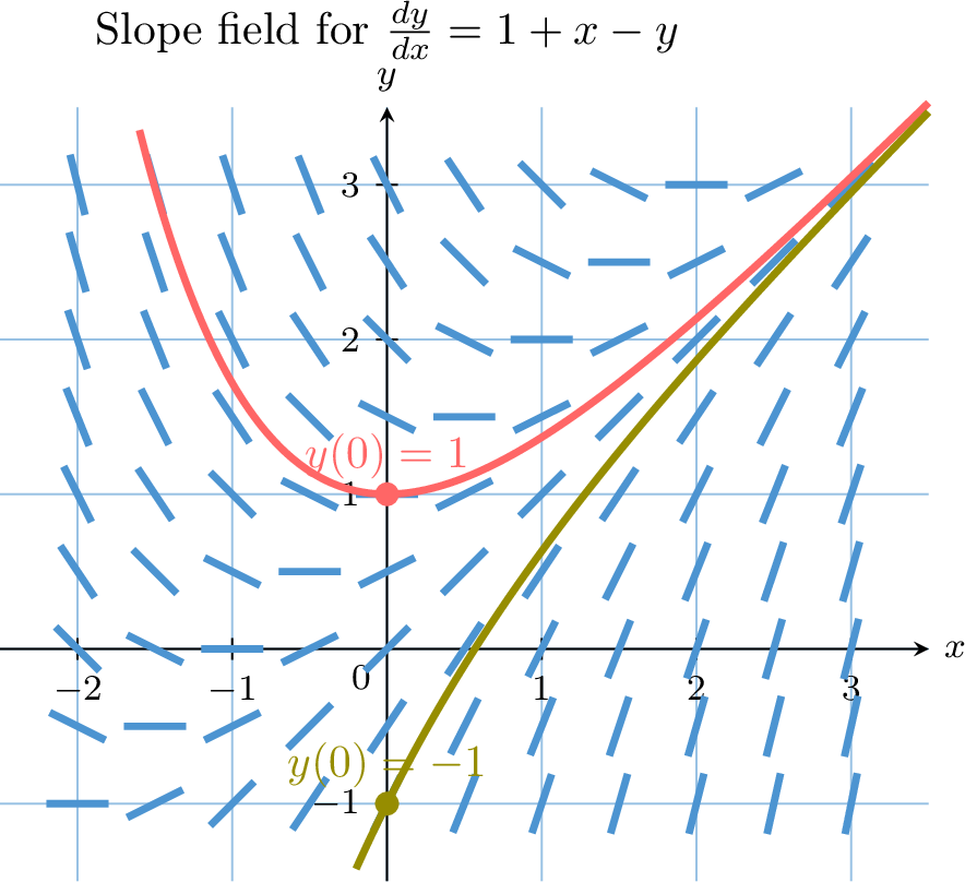
A slope field (or direction field) is a graphical representation of this information. At each point on a grid, we draw a small line segment with the slope given by the differential equation. The resulting field of slopes acts like a set of ``currents'' in a river. Any particular solution to the differential equation is a curve that ``flows'' along these currents, always tangent to the slope markers it passes through.
Method Sketching a Slope Field
To sketch a slope field for \(\dfrac{dy}{dx} = f(x, y)\):
- Choose grid points: Select a representative set of integer points \((x, y)\) in the desired viewing window.
- Calculate slopes: For each point, calculate the value of the slope \(m = f(x, y)\). Organize these values in a table.
- Sketch segments: At each grid point, draw a short line segment with the calculated slope.
Example
For the differential equation \(\dfrac{dy}{dx} = x-y\):
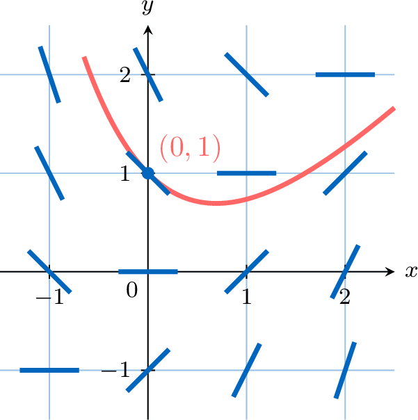
- Sketch the slope field for integer coordinates where \(-1 \le x \le 2\) and \(-1 \le y \le 2\).
- On your sketch, draw the particular solution curve that passes through the point \((0,1)\).
- Sketching the field: We first calculate the slopes \(m=x-y\) at each integer point in the grid.
\(\begin{aligned} & x\\ y \end{aligned} \) -1 0 1 2 2 -3 -2 -1 0 1 -2 -1 0 1 0 -1 0 1 2 -1 0 1 2 3 - Drawing the solution curve: Starting at the initial point \((0,1)\), we follow the direction of the slope field. The curve will be tangent to the line segments as it passes through the field.
Solving by Direct Integration
Method Solving for \(\frac{dy}{dx} \equal f(x)\)
When the derivative of a function depends only on \(x\), we can find the general solution by rearranging the equation and integrating directly.$$\begin{aligned}\frac{dy}{dx} &= f(x)\\
dy &= f(x)\, dx \\
\int dy &= \int f(x) \, dx \\
y &= \int f(x) \, dx + C\end{aligned}$$
Example
Find the general solution to \(\dfrac{dy}{dx} = 3x^2 \) and the particular solution with initial condition \(y(0)=4\).
We rearrange and integrate both sides:$$\begin{aligned}\dfrac{dy}{dx} &= 3x^2 \\
dy &= 3x^2 \, dx \\
\int dy &= \int 3x^2\, dx \\
y & = x^3 + C\end{aligned}$$This is the general solution. Now we use the initial condition \(y(0)=4\):$$ 4 = (0)^3 + C \implies C=4 $$The particular solution is \(y = x^3 + 4\).
Solving by Separation of Variables
A separable differential equation is one that can be expressed in the form \(\dfrac{dy}{dx} = g(x)h(y)\). These equations can be solved by algebraically separating the variables before integrating.
Method Solving Separable Equations \(\frac{dy}{dx} \equal g(x)h(y)\)
This method applies when the equation can be rearranged so that all terms involving \(y\) are on one side and all terms involving \(x\) are on the other.
- Separate: Rearrange the equation into the form \(\dfrac{1}{h(y)}\, dy = g(x)\, dx\).
- Integrate: Integrate both sides of the equation with respect to their respective variables:$$ \int \dfrac{1}{h(y)} \, dy = \int g(x) \, dx $$
- Solve for \(y\): If possible, solve the resulting equation for \(y\) to get an explicit solution.
Example
Solve \(\dfrac{dy}{dx} = -2xy^2\) with the initial condition \(y(1)=1\).
We rearrange and integrate both sides:$$\begin{aligned}\dfrac{dy}{dx} &= -2xy^2 \\
\frac{1}{y^2} \, dy &= -2x \, dx \\
\int \frac{1}{y^2} \, dy &= \int -2x \, dx \\
\int y^{-2} \, dy &= \int -2x \, dx \\
-y^{-1} &= -x^2 + C \\
-\frac{1}{y} &= -x^2 + C\end{aligned}$$This is the general solution in implicit form. Using the initial condition \(y(1)=1\):$$ -\dfrac{1}{1} = -(1)^2 + C \implies -1 = -1 + C \implies C = 0 $$Substituting \(C=0\) gives the particular solution:$$ -\dfrac{1}{y} = -x^2 \implies y = \dfrac{1}{x^2} $$
Solving Homogeneous Equations
A special class of first-order differential equations are those that can be expressed as a function of the ratio \(y/x\). These are known as homogeneous differential equations:$$ \dfrac{dy}{dx} = F\left(\frac{y}{x}\right). $$
Method Solving Homogeneous Equations
To solve a homogeneous differential equation:
- Confirm homogeneity: Rewrite the equation to show it is of the form \(\dfrac{dy}{dx} = F(y/x)\).
- Substitute: Let \(y=vx\). Replace all instances of \(y/x\) with \(v\) and replace \(\dfrac{dy}{dx}\) with \(v + x\dfrac{dv}{dx}\).
- Solve the separable equation: The resulting equation will be separable in terms of \(v\) and \(x\). Solve it for \(v\).
- Back-substitute: Replace \(v\) with \(y/x\) to express the final solution in terms of \(x\) and \(y\).
Example
Find the general solution to the differential equation \(\dfrac{dy}{dx} = \dfrac{x+y}{x}\).
- Confirm homogeneity: We rewrite the right-hand side:$$ \dfrac{dy}{dx} = \frac{x}{x} + \frac{y}{x} = 1 + \frac{y}{x}. $$This is of the form \(F(y/x)\), so it is homogeneous.
- Substitute: Let \(y=vx\). Then \(\dfrac{dy}{dx} = v + x\dfrac{dv}{dx}\). The equation becomes:$$ v + x\dfrac{dv}{dx} = 1 + v. $$
- Solve the separable equation: Now, we solve the new equation for \(v\):$$ x\dfrac{dv}{dx} = 1. $$This is a simple separable equation:$$ dv = \frac{1}{x} \, dx. $$Integrate both sides:$$ \int dv = \int \frac{1}{x} \, dx \implies v = \ln|x| + C. $$
- Back-substitute: Replace \(v\) with \(y/x\) to get the final solution:$$ \frac{y}{x} = \ln|x| + C. $$The explicit general solution is:$$ y = x(\ln|x| + C). $$
Solving with the Integrating Factor
Separable equations are not the only type of first-order differential equation. Consider an equation in the linear form \(\dfrac{dy}{dx} + P(x)y = Q(x)\). We cannot separate the variables here.
The goal is to transform the left side, \(\dfrac{dy}{dx} + P(x)y\), into the result of the product rule for differentiation, \(\dfrac{d}{dx}(I(x)y)\). Recall that the product rule gives:$$ \dfrac{d}{dx}(I(x)y) = I(x)\dfrac{dy}{dx} + I'(x)y. $$Let's try to achieve this by multiplying our original equation by some (currently unknown) function \(I(x)\), which we call the integrating factor:$$ \underbrace{I(x)\dfrac{dy}{dx} + I(x)P(x)y}_{\text{Our transformed left side}} = I(x)Q(x). $$Now, compare the left side to the product rule expansion. For them to be equal, we need:$$ I'(x)y = I(x)P(x)y \implies I'(x) = I(x)P(x). $$This is a separable differential equation for \(I(x)\):$$ \dfrac{I'(x)}{I(x)} = P(x) \implies \int \dfrac{1}{I} \, dI = \int P(x) \, dx \implies \ln|I| = \int P(x) \, dx. $$Solving for \(I(x)\) gives us the formula for the integrating factor: \(I(x) = e^{\int P(x)\, dx}\). By multiplying our original equation by this specific function, we force the left side to become a simple derivative, which we can then easily integrate.
The goal is to transform the left side, \(\dfrac{dy}{dx} + P(x)y\), into the result of the product rule for differentiation, \(\dfrac{d}{dx}(I(x)y)\). Recall that the product rule gives:$$ \dfrac{d}{dx}(I(x)y) = I(x)\dfrac{dy}{dx} + I'(x)y. $$Let's try to achieve this by multiplying our original equation by some (currently unknown) function \(I(x)\), which we call the integrating factor:$$ \underbrace{I(x)\dfrac{dy}{dx} + I(x)P(x)y}_{\text{Our transformed left side}} = I(x)Q(x). $$Now, compare the left side to the product rule expansion. For them to be equal, we need:$$ I'(x)y = I(x)P(x)y \implies I'(x) = I(x)P(x). $$This is a separable differential equation for \(I(x)\):$$ \dfrac{I'(x)}{I(x)} = P(x) \implies \int \dfrac{1}{I} \, dI = \int P(x) \, dx \implies \ln|I| = \int P(x) \, dx. $$Solving for \(I(x)\) gives us the formula for the integrating factor: \(I(x) = e^{\int P(x)\, dx}\). By multiplying our original equation by this specific function, we force the left side to become a simple derivative, which we can then easily integrate.
Method The Integrating Factor Method
This method solves first-order linear differential equations.
- Standard form: Ensure the equation is in the form \(\dfrac{dy}{dx} + P(x)y = Q(x)\).
- Find the integrating factor (I.F.): Calculate \(I(x) = e^{\int P(x)\, dx}\). (No constant of integration is needed here.)
- Multiply: Multiply the entire standard-form equation by \(I(x)\). The left side will now simplify to \(\dfrac{d}{dx}(I(x)y)\):$$ \dfrac{d}{dx}(I(x)y) = I(x)Q(x). $$
- Integrate and solve: Integrate both sides with respect to \(x\) and solve for \(y\):$$ I(x)y = \int I(x)Q(x) \, dx. $$
Example
Solve \(\dfrac{dy}{dx} + 2y = 6\).
The equation is in standard form with \(P(x) = 2\) and \(Q(x) = 6\).
- Find the integrating factor:$$ I(x) = e^{\int 2 \, dx} = e^{2x}. $$
- Multiply by I.F.:$$ e^{2x}\dfrac{dy}{dx} + 2e^{2x}y = 6e^{2x}. $$The left side now equals \(\dfrac{d}{dx}(e^{2x}y)\):$$ \dfrac{d}{dx}(e^{2x}y) = 6e^{2x}. $$
- Integrate and solve:$$ e^{2x}y = \int 6e^{2x} \, dx = \frac{6e^{2x}}{2} + C = 3e^{2x} + C. $$Finally, divide by \(e^{2x}\) to solve for \(y\):$$ y = \frac{3e^{2x} + C}{e^{2x}} = 3 + Ce^{-2x}. $$
Finding Series Solutions of Differential Equations
It is possible to generate the terms of a Maclaurin series for the solution of a differential equation directly from the equation itself, without first finding the solution.
Method Finding a Maclaurin Series from a Differential Equation
Given \(\dfrac{dy}{dx} = f(x,y)\) and an initial condition \(y(0)=y_0\):
- Iterative derivation: Find expressions for the higher derivatives by repeatedly differentiating the equation from the previous step with respect to \(x\). This often requires implicit differentiation.$$\begin{aligned}y' &= f(x,y)\\ y'' &= \frac{d}{dx}f(x,y)\\ y''' &= \frac{d}{dx}\left(\frac{d}{dx}f(x,y)\right)\\ &\vdots\end{aligned}$$
- Iterative substitution: Use the initial condition \((0,y_0)\) and previously found derivative values to find the numerical values of \(y'(0), y''(0), y'''(0), \dots\) in sequence.
- Construct the series: Substitute these values into the Maclaurin series formula:$$ y(x) = y(0) + y'(0)x + \dfrac{y''(0)}{2!}x^2 + \dfrac{y'''(0)}{3!}x^3 + \dots $$
Example
Given \(\dfrac{dy}{dx} = x - 2y\) and \(y(0) = 1\), find the Maclaurin series for \(y(x)\) up to the term in \(x^3\).
We are given \(y(0)=1\).
- Iterative derivation:$$\begin{aligned}y' &= x - 2y\\ y'' &= \frac{d}{dx}(x - 2y) = 1 - 2y'\\ y''' &= \frac{d}{dx}(1 - 2y') = -2y''\end{aligned}$$
- Iterative substitution:$$\begin{aligned}y'(0) &= 0 - 2y(0) = -2(1) = -2,\\ y''(0) &= 1 - 2y'(0) = 1 - 2(-2) = 5,\\ y'''(0) &= -2y''(0) = -2(5) = -10.\end{aligned}$$
- Construct the series:$$\begin{aligned}y(x) &= y(0) + y'(0)x + \dfrac{y''(0)}{2!}x^2 + \dfrac{y'''(0)}{3!}x^3 + \dots \\ &= 1 + (-2)x + \dfrac{5}{2!}x^2 + \dfrac{-10}{3!}x^3 + \dots\\ &= 1 - 2x + \dfrac{5}{2}x^2 - \dfrac{5}{3}x^3 + \dots\end{aligned}$$
Approximating Solutions with Euler's Method
When a differential equation cannot be solved analytically, we can approximate its solution using numerical methods. Euler's method is the simplest of these, using linear approximation to step along the solution curve.
The method begins with an initial condition \((x_0, y_0)\) and proceeds in steps. Let's define a small, constant step size, \(h\). The \(x\)-coordinate of each subsequent point is found by adding this step size: \(x_{n+1} = x_n + h\).
The core of the method is to approximate the derivative \(\dfrac{dy}{dx}\) using the gradient of the line segment connecting two consecutive points, \((x_n, y_n)\) and \((x_{n+1}, y_{n+1})\):$$ \dfrac{dy}{dx} \text{ at } (x_n, y_n) \approx \dfrac{y_{n+1} - y_n}{x_{n+1} - x_n} = \dfrac{y_{n+1} - y_n}{h}. $$Since the differential equation gives us the exact value of the derivative, \(\dfrac{dy}{dx} = f(x_n, y_n)\), we can set these equal:$$ \dfrac{y_{n+1} - y_n}{h}\approx f(x_n, y_n). $$Rearranging this formula to find the next \(y\)-value, \(y_{n+1}\), gives the iterative step:$$ y_{n+1} \approx y_n + h \cdot f(x_n, y_n). $$The collection of line segments created by this iterative procedure forms a polygonal approximation to the true solution curve.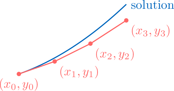
Method Euler's Method
To approximate the solution to \(\dfrac{dy}{dx} = f(x,y)\) with initial condition \((x_0, y_0)\) and a step size \(h\), the coordinates of the next point \((x_{n+1}, y_{n+1})\) are found from the previous point \((x_n, y_n)\) using the iterative formulas:$$\begin{cases}x_{n+1} = x_n + h, \\
y_{n+1} = y_n + h \cdot f(x_n, y_n).\end{cases}$$
Proposition Accuracy and Error
Euler's method is an approximation. The accuracy of this approximation depends on two main factors:
- Step size (\(h\)): A smaller step size \(h\) generally leads to a more accurate approximation. As \(h \to 0\), the polygonal path of the approximation gets closer to the true solution curve. However, this comes at the cost of requiring more computational steps.
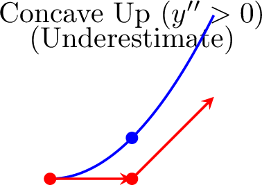
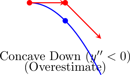
- Concavity of the solution curve: The nature of the curve's concavity determines whether the approximation is an overestimate or an underestimate.
- If the curve is concave up (\(\frac{d^2y}{dx^2} > 0\)), the tangent line at the start of each step lies below the curve. This means Euler's method will consistently produce an underestimate.
- If the curve is concave down (\(\frac{d^2y}{dx^2} < 0\)), the tangent line lies above the curve, resulting in an overestimate.
- If the curve is concave up (\(\frac{d^2y}{dx^2} > 0\)), the tangent line at the start of each step lies below the curve. This means Euler's method will consistently produce an underestimate.
Example
Consider the differential equation \(\dfrac{dy}{dx} = -2xy\) with the initial condition \(y(0)=1\).
- Use Euler's method with a step size of \(h=0.1\) to find an approximate value for \(y(0.2)\).
- By solving the differential equation, show that the particular solution is \(y(x) = e^{-x^2}\).
- Calculate the percentage error in your approximation from part (a).
- By considering the sign of \(\dfrac{d^2y}{dx^2}\) in the interval \(0 \le x \le 0.2\), explain whether your approximation in part (a) is an overestimate or an underestimate of the true value.
- We start at \((x_0, y_0)=(0,1)\) with \(h=0.1\) and \(f(x,y)=-2xy\).
- Step 1: \(y_1 = y_0 + h \cdot (-2x_0y_0) = 1 + 0.1(-2\cdot 0 \cdot 1) = 1\). So, \(y(0.1) \approx 1\).
- Step 2: \(y_2 = y_1 + h \cdot (-2x_1y_1) = 1 + 0.1(-2\cdot 0.1 \cdot 1) = 1 - 0.02 = 0.98\).
- We solve by separating variables:$$ \frac{dy}{dx} = -2xy \implies \int \frac{1}{y} \, dy = \int -2x \, dx. $$Thus$$ \ln|y| = -x^2 + C. $$Using the initial condition \(y(0)=1\):$$ \ln|1| = -0^2 + C \implies C=0. $$So, \(\ln y = -x^2\) (since \(y(0)=1>0\)), which gives the particular solution \(y(x) = e^{-x^2}\).
- The exact value is \(y_{\text{exact}} = e^{-(0.2)^2} = e^{-0.04} \approx 0.960789\ldots\) The approximate value is \(y_{\text{approx}} = 0.98\). The percentage error is$$ \text{Error} = \left|\frac{0.960789\ldots - 0.98}{0.960789\ldots}\right| \times 100\pourcent \approx 2.00\pourcent. $$
- To determine the nature of the error, we check the concavity by finding the second derivative:$$\begin{aligned}\frac{d^2y}{dx^2} &= \frac{d}{dx}(-2xy) \\ &= -2\left(1 \cdot y + x \cdot \frac{dy}{dx}\right) \\ &= -2\bigl(y + x(-2xy)\bigr) \\ &= -2y(1-2x^2).\end{aligned}$$At the start of the approximation, for \(x\) in \([0, 0.2]\), \(x^2\) is small, so \((1-2x^2)\) is positive. Since \(y\) is also positive in this region, the sign of the second derivative is$$ \frac{d^2y}{dx^2} = (\text{negative})\times(\text{positive})\times(\text{positive}) < 0. $$Since the second derivative is negative, the solution curve is concave down. Euler's method uses the tangent line to approximate the curve. For a concave down function, the tangent line lies above the curve. Therefore, each step of the approximation will land on a point higher than the actual curve, making it an overestimate.