Sampling and Confidence Intervals
Statistical Modeling
In most real-world statistical problems, we are interested in understanding the properties of a large population. However, it is often impossible or impractical to collect data from every single member of that population. As a result, we typically do not know the true population parameters, such as the population mean (\(\mu\)) or the population standard deviation (\(\sigma\)).
Instead, we collect data from a smaller subset of the population, called a sample. We calculate statistics from this sample (like the sample mean \(\bar{x}\)) and use them to estimate the unknown population parameters. This process is known as statistical inference. In this section, we will define the key concepts used in sampling and estimation.
Instead, we collect data from a smaller subset of the population, called a sample. We calculate statistics from this sample (like the sample mean \(\bar{x}\)) and use them to estimate the unknown population parameters. This process is known as statistical inference. In this section, we will define the key concepts used in sampling and estimation.
Definition Sample
A sample of size \(n\) consists of \(n\) independent random variables \(X_1, X_2, \dots, X_n\) that follow the same probability distribution as the population.
Definition Observed Value
An observed value, denoted by a lowercase \(x\), is a specific realization of a random variable \(X\). It is the actual number obtained after performing an experiment or collecting data.
Definition Sample Mean Estimator
The sample mean is a statistic used to estimate the population mean.
Let \(X_1, X_2, \dots, X_n\) be a random sample. The sample mean is a random variable denoted by \(\overline{X}_n\):$$ \overline{X}_n = \frac{\sum_{i=1}^n X_i}{n} = \frac{X_1 + X_2 + \dots + X_n}{n} $$For a specific set of observed values \(x_1, x_2, \dots, x_n\), the calculated sample mean is denoted by \(\bar{x}\):$$ \bar{x} = \frac{\sum_{i=1}^n x_i}{n} $$
Let \(X_1, X_2, \dots, X_n\) be a random sample. The sample mean is a random variable denoted by \(\overline{X}_n\):$$ \overline{X}_n = \frac{\sum_{i=1}^n X_i}{n} = \frac{X_1 + X_2 + \dots + X_n}{n} $$For a specific set of observed values \(x_1, x_2, \dots, x_n\), the calculated sample mean is denoted by \(\bar{x}\):$$ \bar{x} = \frac{\sum_{i=1}^n x_i}{n} $$
Proposition Unbiased Estimator of the Mean
The sample mean is an unbiased estimator of the population mean \(\mu\). This means that the expected value of the sample mean is equal to the true population mean:$$ E[\overline{X}_n] = \mu $$
Definition Sample Standard Deviation
The sample standard deviation, denoted by \(s_n\) (or simply \(s\)), is an estimator of the population standard deviation \(\sigma\). For observed values \(x_1, x_2, \dots, x_n\):$$ s_n = \sqrt{\frac{\sum_{i=1}^n (x_i - \bar{x})^2}{n-1}} $$Note the division by \(n-1\) (Bessel's correction), which ensures that the associated sample variance \(s_n^2\) is an unbiased estimator of the population variance.
Proposition Unbiased Estimator of the Variance
The sample variance \(S_n^2 = \frac{\sum (X_i - \overline{X}_n)^2}{n-1}\) is an unbiased estimator of the population variance \(\sigma^2\):$$ E[S_n^2] = \sigma^2 $$
Example Survey: Do you like Mathematics?
For an education survey, 10 students rate how much they like mathematics on a scale of 0 to 10.Let \(X_1, X_2, \dots, X_{10}\) be the random variables representing the rating of each student.The observed values are: \(x = \{2, 4, 0, 9, 10, 3, 7, 2, 8, 9\}\).
- Sample Mean: $$ \bar{x} = \frac{2+4+0+9+10+3+7+2+8+9}{10} = \frac{54}{10} = 5.4 $$
- Sample Standard Deviation: Using a calculator (List statistics): $$ s_{n} \approx 3.50 $$
Confidence Intervals for Means with Known Variance
A point estimate, like the sample mean \(\bar{x}\), provides a single value as an estimate of the population parameter. However, it does not tell us how precise this estimate is. Due to sampling variability, \(\bar{x}\) is rarely exactly equal to the true mean \(\mu\).
To address this, we use a confidence interval. A confidence interval provides a range of values within which we expect the true population parameter to lie, with a certain level of confidence (probability). In this section, we assume that the population variance \(\sigma^2\) is known, which allows us to use the standard normal distribution (\(Z\)).
To address this, we use a confidence interval. A confidence interval provides a range of values within which we expect the true population parameter to lie, with a certain level of confidence (probability). In this section, we assume that the population variance \(\sigma^2\) is known, which allows us to use the standard normal distribution (\(Z\)).
Proposition Probability Interval
Assume we take a sample of size \(n\) from a population with mean \(\mu\) and standard deviation \(\sigma\), and that \(n\) is sufficiently large (typically \(n \ge 30\) so that the Central Limit Theorem applies). Then$$ P\left(\overline{X}_n - 1.96 \frac{\sigma}{\sqrt{n}} \leqslant \mu \leqslant \overline{X}_n + 1.96 \frac{\sigma}{\sqrt{n}}\right) = 0.95. $$
Since \(n\) is large, the Central Limit Theorem applies. The sampling distribution of the mean \(\overline{X}_n\) is approximately normal with mean \(\mu\) and standard deviation \(\dfrac{\sigma}{\sqrt{n}}\).
The standardized variable \(Z\) follows a standard normal distribution:$$ Z = \frac{\overline{X}_n - \mu}{\sigma/\sqrt{n}} \sim N(0, 1). $$For a \(95\pourcent\) confidence level, we seek the critical value \(z\) such that \(P(-z \leqslant Z \leqslant z) = 0.95\).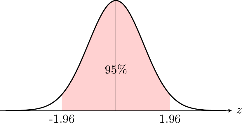
The standardized variable \(Z\) follows a standard normal distribution:$$ Z = \frac{\overline{X}_n - \mu}{\sigma/\sqrt{n}} \sim N(0, 1). $$For a \(95\pourcent\) confidence level, we seek the critical value \(z\) such that \(P(-z \leqslant Z \leqslant z) = 0.95\).
The proposition above gives us a probability statement about the random sample mean \(\overline{X}_n\) and the random interval built from it. The parameter \(\mu\) is fixed (but unknown); what is random is the interval itself.
To calculate a specific confidence interval in practice, we estimate this probability interval by replacing the random variable \(\overline{X}_n\) with the observed sample mean \(\bar{x}\). Thus, the confidence interval we compute is an estimate of the theoretical interval.
To calculate a specific confidence interval in practice, we estimate this probability interval by replacing the random variable \(\overline{X}_n\) with the observed sample mean \(\bar{x}\). Thus, the confidence interval we compute is an estimate of the theoretical interval.
Method Calculating the Confidence Interval (Mean)
- Identify the statistics: Find the sample mean \(\bar{x}\), the known population standard deviation \(\sigma\), and the sample size \(n\).
- Find the z-score: Determine \(z\) based on the confidence level (1.645 for 90\(\pourcent\), 1.96 for 95\(\pourcent\), 2.576 for 99\(\pourcent\)).
- Calculate the margin of error: \(E = z \dfrac{\sigma}{\sqrt{n}}\).
- Write the interval: \([\bar{x} - E, \bar{x} + E]\).
Example
A sample of 60 rabbits was taken from a forest. The sample mean weight of the rabbits was \(950\) grams. Assume the population standard deviation is known to be \(\sigma = 200\) grams.
Find the \(95\pourcent\) confidence interval for the population mean weight.
Find the \(95\pourcent\) confidence interval for the population mean weight.
- Statistics: \(n=60\), \(\bar{x}=950\), and \(\sigma=200\).
- z-score: For \(95\pourcent\), \(z = 1.96\).
- Margin of error: $$ E = 1.96 \times \frac{200}{\sqrt{60}} \approx 1.96 \times 25.82 \approx 50.6. $$
- Interval: $$ [950 - 50.6, \ 950 + 50.6] = [899.4, 1000.6]. $$
Confidence Intervals for Means with Unknown Variance
In most practical situations, the population standard deviation \(\sigma\) is unknown. We cannot use the normal distribution (\(Z\)) with a known \(\sigma\), because we must estimate \(\sigma\) using the sample standard deviation \(s_n\).
In theory, when the population is normal and \(\sigma\) is unknown, the exact sampling distribution of$$ \frac{\overline{X}_n - \mu}{S_n/\sqrt{n}} $$is a Student's t-distribution with \(n-1\) degrees of freedom. For large samples (say \(n \ge 30\)), the t-distribution is very close to the standard normal distribution. In this course, for large \(n\), we will approximate by using the same \(z\)-values as before and replacing \(\sigma\) with \(s_n\).
In theory, when the population is normal and \(\sigma\) is unknown, the exact sampling distribution of$$ \frac{\overline{X}_n - \mu}{S_n/\sqrt{n}} $$is a Student's t-distribution with \(n-1\) degrees of freedom. For large samples (say \(n \ge 30\)), the t-distribution is very close to the standard normal distribution. In this course, for large \(n\), we will approximate by using the same \(z\)-values as before and replacing \(\sigma\) with \(s_n\).
Method Calculating the Confidence Interval (Unknown \(\sigma\), Large \(n\))
- Identify the statistics: Find the sample mean \(\bar{x}\), the sample standard deviation \(s_n\) (as an estimate for \(\sigma\)), and the sample size \(n\).
- Find the z-score: Determine \(z\) based on the confidence level (1.645 for 90\(\pourcent\), 1.96 for 95\(\pourcent\), 2.576 for 99\(\pourcent\)), provided \(n\) is large.
- Calculate the margin of error: \(E = z \dfrac{s_n}{\sqrt{n}}\).
- Write the interval: \([\bar{x} - E, \bar{x} + E]\).
Example
An economist studying fuel costs wants to estimate the mean price of gasoline in her state. She takes a random sample of 40 gas stations and finds a sample mean price of \(\bar{x} = \dollar 1.29\) with a sample standard deviation of \(s_n = \dollar 0.10\).
Find the \(95\pourcent\) confidence interval for the population mean.
Find the \(95\pourcent\) confidence interval for the population mean.
- Statistics: \(n=40\), \(\bar{x}=1.29\), and \(s_n=0.10\). (Since \(n \ge 30\), we approximate \(\sigma \approx s_n\).)
- z-score: For \(95\pourcent\), \(z = 1.96\).
- Margin of error: $$ E = 1.96 \times \frac{0.10}{\sqrt{40}} \approx 1.96 \times 0.0158 \approx 0.031. $$
- Interval: $$ [1.29 - 0.031, \ 1.29 + 0.031] = [1.259, 1.321]. $$
Confidence Intervals for Proportions
When dealing with categorical data (like voting for Candidate A vs Candidate B), we are interested in the population proportion \(p\) (the true percentage of votes). Since we cannot ask everyone, we estimate \(p\) using the sample proportion \(\hat{p}\).
Each individual response (success/failure) is a Bernoulli random variable with variance \(p(1-p)\) and standard deviation \(\sigma = \sqrt{p(1-p)}\).
Since the sample proportion \(\hat{p}\) is the mean of \(n\) Bernoulli variables, its standard deviation is \(\dfrac{\sigma}{\sqrt{n}}\).
Therefore, the standard error for a proportion is$$ \sqrt{\frac{p(1-p)}{n}}, $$which we estimate using the sample data as$$ \sqrt{\frac{\hat{p}(1-\hat{p})}{n}}. $$This normal approximation works well when the sample size is large, typically when \(n\hat{p} \ge 5\) and \(n(1-\hat{p}) \ge 5\).
Method Constructing the Interval
- Calculate the sample proportion: \(\hat{p} = \dfrac{\text{Successes}}{\text{Total Sample}}\).
- Find the z-score: Determine \(z\) based on the confidence level (1.645 for 90\(\pourcent\), 1.96 for 95\(\pourcent\), 2.576 for 99\(\pourcent\)).
- Calculate the margin of error: \(E = z \sqrt{\dfrac{\hat{p}(1-\hat{p})}{n}}\).
- Write the interval: \([\hat{p} - E, \hat{p} + E]\).
Example
A polling institute surveys \(n=1000\) random voters before an election. 520 people say they will vote for Candidate A.
- Calculate the sample proportion \(\hat{p}\).
- Construct a \(95\pourcent\) confidence interval for the true proportion of voters supporting Candidate A.
- Based on this interval, can Candidate A be certain of winning (obtaining more than \(50\pourcent\) of votes)? Explain.
- \(\hat{p} = \dfrac{520}{1000} = 0.52\).
- Using the 95\(\pourcent\) confidence level (\(z=1.96\)): $$ \begin{aligned} E &= 1.96 \sqrt{\frac{0.52(1-0.52)}{1000}} \\ &= 1.96 \sqrt{\frac{0.52 \times 0.48}{1000}} \\ &= 1.96 \sqrt{0.0002496} \\ &= 1.96(0.0158) \\ &\approx 0.031. \end{aligned} $$ The confidence interval is: $$ [0.52 - 0.031, \ 0.52 + 0.031] = [0.489, 0.551] $$ (Or \(48.9\pourcent\) to \(55.1\pourcent\)).
- No. Although the sample proportion is \(52\pourcent\), the interval includes values less than \(0.5\) (e.g., \(0.489\)). Therefore, it is plausible that the true proportion is below \(50\pourcent\). The election is too close to call with certainty.
Hypothesis Testing using Confidence Intervals
Confidence intervals can be used as a tool for hypothesis testing. If someone claims that the population mean is a specific value (\(\mu_H\)), we can check if this value is ``plausible'' by seeing whether it falls within our calculated confidence interval.
For a two-sided test at significance level \(\alpha\) (e.g.\ \(5\pourcent\)), the \((1-\alpha)\) confidence interval (e.g.\ \(95\pourcent\)) gives the same decision as the corresponding hypothesis test \(H_0 : \mu = \mu_H\) versus \(H_1 : \mu \neq \mu_H\).
For a two-sided test at significance level \(\alpha\) (e.g.\ \(5\pourcent\)), the \((1-\alpha)\) confidence interval (e.g.\ \(95\pourcent\)) gives the same decision as the corresponding hypothesis test \(H_0 : \mu = \mu_H\) versus \(H_1 : \mu \neq \mu_H\).
Method Hypothesis Test with CI
To test a claim that the population mean is \(\mu_H\) at a significance level \(\alpha\) (e.g., \(5\pourcent\)):
- Construct the corresponding \((1-\alpha)\) confidence interval (e.g., \(95\pourcent\)) for \(\mu\) based on sample data.
- Decision rule:
- If \(\mu_H\) is inside the interval, we do not reject the claim (the claim is plausible).
- If \(\mu_H\) is outside the interval, we reject the claim (the result is statistically significant at level \(\alpha\)).
Example
A machine is set to fill juice bottles with an average of \(50 \mathrm{cl}\). A quality control inspector takes a sample of 36 bottles and finds an average content of \(48.5 \mathrm{cl}\) with a standard deviation of \(5 \mathrm{cl}\).
Test the claim that the machine average is still \(50 \mathrm{cl}\) at the 5\(\pourcent\) significance level, using a \(95\pourcent\) confidence interval for \(\mu\).
Test the claim that the machine average is still \(50 \mathrm{cl}\) at the 5\(\pourcent\) significance level, using a \(95\pourcent\) confidence interval for \(\mu\).
Sample size \(n=36\), \(\bar{x}=48.5\), \(s_n=5\). Since \(n\) is reasonably large, we use a normal approximation with \(z=1.96\).We construct the \(95\pourcent\) confidence interval for the true mean \(\mu\):$$ \begin{aligned}CI &= 48.5 \pm 1.96 \frac{5}{\sqrt{36}} \\
&= 48.5 \pm 1.96 \left(\frac{5}{6}\right) \\
&= 48.5 \pm 1.633 \\
&= [46.87, 50.13].\end{aligned} $$Conclusion: The claimed value \(\mu_H = 50\) lies inside the confidence interval \([46.87, 50.13]\). Therefore, we do not reject the claim at the 5\(\pourcent\) level. There is not enough evidence to say the machine is malfunctioning based on this sample.
Determining Sample Size
Before conducting a study, researchers often need to know how many data points to collect to achieve a desired level of precision. By manipulating the formula for the margin of error, we can solve for the required sample size \(n\) (for example, when estimating a mean with known standard deviation \(\sigma\)).
Proposition Sample Size Formula
To estimate a population mean within a margin of error \(E\) with a specific confidence level (corresponding to \(z\)), when \(\sigma\) is known, the required sample size is:$$ n = \left( \frac{z \sigma}{E} \right)^2. $$Note: Since \(n\) must be an integer, always round up to the next whole number.
Starting from the margin of error definition:$$ E = z \frac{\sigma}{\sqrt{n}} $$we rearrange:$$ \sqrt{n} E = z \sigma $$$$ \sqrt{n} = \frac{z \sigma}{E} $$$$ n = \left( \frac{z \sigma}{E} \right)^2. $$
Example
A marketing firm wants to estimate the average spending of students during Spring Break. They want the estimate to be within \(\dollar 120\) of the true mean with \(90\pourcent\) confidence. A pilot study suggests the standard deviation is \(\sigma = \dollar 400\). How many students should be sampled?
Given:
Result: A sample of size \(n=31\) is required.
- Margin of error \(E = 120\)
- Standard deviation \(\sigma = 400\)
- Confidence level \(90\pourcent \implies z \approx 1.645\) (from calculator or tables)
Result: A sample of size \(n=31\) is required.